Z Pinch Kinetics II - A Continuum Perspective: Betatron Heating and Self-Generation of Sheared Flows

Doubly adiabatic CGL theory describes collisionless compression of magnetized plasma, and predicts different degrees of parallel and perpendicular heating due to magnetic flux compression Chew, Goldberger, and Low (1956). The classic CGL model consists of two invariants, one for each pressure component

	$\displaystyle\frac{d}{dt}\Big{(}\frac{p_{\perp}}{\rho B}\Big{)}$	$\displaystyle=$	$\displaystyle 0,$		(4a)
	$\displaystyle\frac{d}{dt}\Big{(}\frac{p_{\parallel}B^{2}}{\rho^{3}}\Big{)}$	$\displaystyle=$	$\displaystyle 0,$		(4b)

in contrast to the singly adiabatic (conserved specific entropy) invariant $\frac{d}{dt}\big{(}\frac{p}{\rho^{\gamma}}\big{)}=0$.

Equations 4 hold in the cylindrical Z pinch for fluid elements which are made up primarily of cyclotron trajectories. This is demonstrated simply as follows. Suppose that a plasma fluid element is characterized by three adiabatic invariants, namely specific magnetic moment $\mu$, specific angular momentum $L_{\theta}$, and specific magnetic flux $s_{m}$ (from Alfvén’s law)

	$\displaystyle\frac{d\mu}{dt}=0$	$\displaystyle\quad\implies\quad$	$\displaystyle\frac{d}{dt}\Big{(}\frac{v_{\mathrm{th},\perp}^{2}}{B_{\theta}}\Big{)}=0,$		(5a)
	$\displaystyle\frac{dL_{\theta}}{dt}=0$	$\displaystyle\quad\implies\quad$	$\displaystyle\frac{d}{dt}(rv_{\mathrm{th},\parallel})=0,$		(5b)
	$\displaystyle\frac{ds_{m}}{dt}=0$	$\displaystyle\quad\implies\quad$	$\displaystyle\frac{d}{dt}\Big{(}\frac{B_{\theta}}{\rho r}\Big{)}=0$		(5c)

where $v_{\mathrm{th},\parallel}=\sqrt{k_{B}T_{\parallel}/m}$ is the parallel thermal velocity and $v_{\mathrm{th},\perp}=\sqrt{k_{B}T_{\perp}/m}$ the perpendicular one. Then substituting the parallel and perpendicular pressures ($p_{\parallel}=nkT_{\parallel}$ and $p_{\perp}=nkT_{\perp}$) for the thermal velocities and combining Eqs. 5 yields exactly Eqs. 4, the CGL equations.

Equations 5 clarify the double-adiabatic CGL model in cylindrical geometry as consisting of the magnetic moment plus the angular momentum invariant, versus the Cartesian picture in which the second invariant is the mirror bounce action $J_{\parallel}\sim v_{\parallel}\ell$ along a field-aligned path of length $\ell$. The singly adiabatic model (invariant specific entropy) arises in the collisional limit $\omega_{ci}\tau\ll 1$. Observe that the CGL model is truly triply adiabatic considering the necessity of Alfvén’s law to obtain the CGL equations and the thermodynamic character of the specific magnetic flux Crews et al. (2024).

Compression in the Cartesian slab model and in the cylindrical pinch are distinguished by the Jacobian appearing in Alfvén’s law Turchi and Shumlak (2023). Namely, the Cartesian slab has $\frac{d}{dt}\big{(}\frac{B}{\rho}\big{)}=0$ while the cylinder has $\frac{d}{dt}\big{(}\frac{B_{\theta}}{\rho r}\big{)}=0$, a subtle difference which can lead to opposite expectations. That is, combining Eqs. 4 with these frozen flux invariants produces the following equations,

	Slab,	$\displaystyle\frac{d}{dt}\Big{(}\frac{p_{\parallel}}{p_{\perp}}B\Big{)}=0,$			(6a)
	Cylinder,	$\displaystyle\frac{d}{dt}\Big{(}\frac{p_{\parallel}}{p_{\perp}}B_{\theta}r^{2}\Big{)}=0.$			(6b)

Cartesian slab anisotropy is simply inversely proportional to the flux compression ratio, $\frac{p_{\parallel,2}}{p_{\perp,2}}=C_{m}^{-1}$ (with $C_{m}\equiv\frac{B_{2}}{B_{1}}$) between an isotropic initial state $(\cdot)_{1}$ and an anisotropic compressed state $(\cdot)_{2}$. In the same vein, anisotropy in the cylinder follows from Eq. 6b as

$$\frac{p_{\parallel,2}}{p_{\perp,2}}=\Big{(}\frac{I_{1}}{I_{2}}\Big{)}\Big{(}\frac{r_{1}}{r_{2}}\Big{)}$$

(7)

where $\mu_{0}I\equiv 2\pi rB_{\theta}$ is the axial current enclosed up to radius $r$.

Thus, the anisotropy produced by flux compression of cyclotron trajectories in a Z pinch is the product of two factors: the current amplification ratio and the ratio of radii (alternatively, the product of the flux and area compression ratios). Flux compression in the Cartesian slab always leads to the anisotropy orientation $p_{\parallel}<p_{\perp}$, but the Z pinch will easily display the orientation $p_{\parallel}>p_{\perp}$ if current does not increase by a greater fraction than the radius. This azimuthal over-heating can happen because angular momentum conservation competes with magnetic moment conservation, and has important consequences for the resulting radial force balance.

To summarize the preceding, fluid elements composed of cyclotron trajectories display two adiabatic invariants (Eqs. 5), magnetic moment and angular momentum, and an additional frozen-in flux invariant. In the cylinder, magnetic moment is the invariant associated with radial and axial bounce of the cyclotron orbit, and the angular momentum with periodic azimuthal orbits.

Idealized betatron trajectories display invariants closely related to those of the ideal cyclotrons with a crucial difference: the lines of electric current are the principal symmetry axis rather than the magnetic field lines. Ergo, fluid elements composed of betatron trajectories should follow the same CGL equations as the cyclotrons, but the notions of parallel and perpendicular refer to the electrical current axis ($\hat{z}$) instead of the magnetic field lines, which we demonstrate below.

The adiabatic invariants of an ideal betatron orbit consist of its radial bounce action $J_{r}$, its axial bounce action $J_{z}$, and its azimuthal angular momentum $L_{\theta}$ (or action of the periodic azimuthal motion). These invariants are inferred from the ideal betatron orbit (cf. the prequel Crews, Meier, and Shumlak (2024)), which we present here for self-completeness.

The radial potential energy of a charged particle in the vicinity of the Z-pinch axis is

$$U=\frac{(P_{z}-q_{s}A_{z})^{2}}{2m_{s}}\approx\frac{P_{z}^{2}}{2m_{s}}-P_{z}\frac{q_{s}A_{z}}{m_{s}}$$

(8)

with $P_{z}$ the z-component of canonical momentum, provided that $P_{z}\gg-\frac{1}{2}q_{s}A_{z}$. Expanding the vector potential to $\mathcal{O}(r^{2})$ around the Z-pinch axis yields a harmonic potential $U\approx\frac{1}{2}kr^{2}$ describing a radial bounce with spring constant $k$. The axial bounce motion follows from conservation of canonical momentum. These radial and axial bounce motions are expressed as

	$\displaystyle r(t)$	$\displaystyle=$	$\displaystyle r_{0}\sin(\omega_{\beta}t),$		(9a)
	$\displaystyle mv_{z}(t)$	$\displaystyle=$	$\displaystyle P_{z}-\kappa\sin^{2}(\omega_{\beta}t).$		(9b)

The axial momentum fluctuation amplitude $\kappa\equiv q_{s}A_{z}(r_{0})$ is the potential momentum at the radial turning point $r_{0}$ and $\omega_{\beta}$ is the betatron frequency with $\omega_{\beta}^{2}\equiv\frac{q_{s}B_{\theta}}{m_{s}}\frac{v_{z}}{r}$. The radial and axial bounce motions contribute substantially to temperature in the species drift frame.

The radial bounce invariant follows as the area of the $(r,v_{r})$ phase-plane orbit,

$$J_{r}=\pi m_{s}r_{0}^{2}\omega_{\beta}\sim v_{r0}r_{0},$$

(10)

or the product of the radial bounce amplitude $r_{0}$ and the radial velocity amplitude $v_{r0}$. The radial bounce action is similar in form to the angular momentum or mirror bounce invariants, i.e. velocity times length, as a simple harmonic motion.

The axial bounce invariant is found by transforming to the bounce-averaged ($\langle\cdot\rangle_{T}$) axial drift frame, i.e. to the oscillation-center coordinates $(\delta z,\delta v_{z})$. The oscillation-center trajectory is

	$\displaystyle\langle m_{s}v_{z}\rangle_{T}$	$\displaystyle=$	$\displaystyle P_{z}-\frac{\kappa}{2},$		(11a)
	$\displaystyle\delta(m_{s}v_{z})\equiv m_{s}v_{z}-\langle m_{s}v_{z}\rangle_{T}$	$\displaystyle=$	$\displaystyle-\kappa\cos(2\omega_{\beta}t),$		(11b)

and the axial bounce invariant as the area of the oscillation-center phase-plane ellipse,

$$J_{z}=\pi\frac{\kappa^{2}/2m_{s}}{\omega_{\beta}}.$$

(12)

Equations 10 and 12 hold approximately for non-ideal betatron orbits, in a similar way that magnetic moment invariance is taken to hold for cyclotron orbits, although it is truly conserved only up to guiding-center corrections. We also consider axis-encircling betatron orbits to be approximately described by Eqs. 10 and 12 with the addition of an angular momentum invariant, $J_{\theta}=m_{s}r_{0}v_{\theta}$, because betatron orbits with azimuthal momentum may be approximated as an in-plane bounce orbit that rotates around the $\hat{z}$-axis Crews, Meier, and Shumlak (2024).

We now specialize to ion trajectories because their orbits are much larger than the electrons. The characteristic betatron frequency $\omega_{\beta}$ follows from $\omega_{\beta}^{2}\equiv\omega_{ci}\frac{v_{z}}{r}$ by setting $v_{z}$ equal to the ion axial drift $v_{i}$ (in the perfectly neutral Lorentz frame). Three useful forms of this frequency are

$$\omega_{\beta}=\frac{v_{\mathrm{th},i}}{r_{p}}=\frac{v_{i}}{\lambda_{i}}=\omega_{ci}\mathfrak{B}_{i}^{-1/2}$$

(13)

where $v_{\mathrm{th},i}$ is ion thermal velocity, $r_{p}$ is pinch radius, $\lambda_{i}=c/\omega_{pi}$ is ion inertial length, $\omega_{ci}$ is characteristic ion cyclotron frequency, and $\mathfrak{B}_{i}$ the ion Budker parameter Crews, Meier, and Shumlak (2024).

Applying Eq. 13 to Eq. 12 and supposing $\mathfrak{B}_{i}=\text{const.}$, we infer three Lagrangian invariants associated to an ion fluid element threaded by betatron orbits, in analogy to Eqs. 5, to be

	$\displaystyle\frac{d}{dt}\Big{(}\frac{v_{\mathrm{th},z}^{2}}{B_{\theta,0}}\Big{)}=0,$		(14a)
	$\displaystyle\frac{d}{dt}(rv_{\mathrm{th},r\theta})=0,$		(14b)
	$\displaystyle\frac{d}{dt}\Big{(}\frac{B_{\theta,0}}{\rho r}\Big{)}=0$		(14c)

having assumed $(r,\theta)$-isotropy, corresponding to the thermal axial invariant (Eq. 14a), radial invariant (Eq. 14b) and azimuthal angular momentum invariant (Eq. 14b). In Eqs. 14, $B_{\theta,0}$ is the characteristic flux density in the vicinity of the magnetic O-point about which the betatron orbits are bouncing. Combination of Eqs. 14 obtains the CGL model for an ion betatron fluid element,

	$\displaystyle\frac{d}{dt}\Big{(}\frac{p_{r\theta}}{\rho B_{\theta,0}}\Big{)}$	$\displaystyle=$	$\displaystyle 0,$		(15a)
	$\displaystyle\frac{d}{dt}\Big{(}\frac{p_{z}B_{\theta,0}^{2}}{\rho^{3}}\Big{)}$	$\displaystyle=$	$\displaystyle 0.$		(15b)

The electrical current axis assumes the principal anisotropy axis of the betatron fluid, and is otherwise modeled by the same CGL equations as a cyclotron plasma fluid. The radial and azimuthal directions display harmonic motions essentialized by a characteristic distance and a characteristic velocity (similar to the longitudinal mirror invariant), and the harmonic motion of the axial direction is essentialized by characteristic kinetic energy and the characteristic cyclotron frequency (like the magnetic moment of the cyclotrons). Anisotropic heating of the radial and axial directions is an intuitive consequence of the inductive axial electric field associated with flux compression splitting its energy between: 1) acceleration of the betatron axial drift, and 2) particle heating through increasing the energy of the betatron’s radial, axial, and azimuthal periodic motions.

Equations 14 come with important caveats. These invariants have been inferred based on the properties of “linear” betatron orbits, for which $P_{z}\gg-q_{s}A_{z}/2$, which translates to a very small trapping parameter in the prequel’s terminology Crews, Meier, and Shumlak (2024). This analysis based on the linear orbit’s invariants parallels invariance of the magnetic moment for the cyclotron trajectories only to lowest order in the finite Larmor radius (FLR) parameter, viz. trapping parameter. The action integrals of a particular orbit are truly nonlinear functions of its trapping parameter.

Indeed, for the Bennett distribution, nonlinearity is non-negligible for many near-axis orbits. Sufficiently close to the magnetic O-point, these adiabatic invariants are expressed in elliptic integrals. Such nonlinear expressions for the radial betatron action were given explicitly by Sonnerup Sonnerup (1971) in the context of a reconnecting current sheet. Sonnerup’s analysis identified a significant fact: adiabatic compression of the center of the current sheet causes all orbits (both cyclotrons and betatrons) to approach the same elliptic modulus (trapping parameter) $\alpha=2^{-1/4}\approx 0.84$ (at constant canonical momentum $P_{z}$). This trapping parameter $\alpha<1$ represents a nonlinear betatron oscillation Crews, Meier, and Shumlak (2024). Thus, a corollary of Sonnerup’s result, originally identified for adiabatic compression of a reconnecting current sheet, is that sufficient flux compression of the Z pinch drives all near-axis particles into a nonlinear betatron orbit.

Sonnerup’s result assumes that the non-adiabatic cyclotron-betatron separatrix crossing is adiabatic-in-mean, as argued by Janicke Janicke (1975). In reality, the separatrix crossing is chaotic, as explored by Cary et al. Cary, Escande, and Tennyson (1986) and Büchner Büchner and Zelenyi (1989), which results in compression timescale-dependent corrections to the spectrum of the resulting betatron orbit flux. We note however that such non-adiabatic cross-separatrix orbital variations are less significant for the compressing Z pinch than the reconnecting current sheet because the infinite-period separatrix only occurs for purely radial/axial bounce orbits. Non-zero angular momentum of axis-encircling orbits erases the infinite-period separatrix, although all trajectories passing directly through $r=0$ may undergo these chaotic non-adiabatic changes. Non-adiabatic transitions across the betatron-cyclotron separatrix of axis-crossing orbits in a compressing Z pinch deserves deeper investigation in a future study.

Sections III.1 and III.2 established that the CGL model applies to plasma composed of either cyclotron or betatron trajectories, in the usual way for the cyclotron plasma and a modified way for the betatron plasma. Specifically, the models predict the same magnitude of anisotropic heating from flux compression of a pinched plasma displaying either flavor of motion, but predict differing principal anisotropy axes; either the magnetic field lines for fluid consisting of cyclotron trajectories, or the electrical current lines for a fluid of betatron trajectories.

We now combine Sections III.1 and III.2 to propose an anisotropy model for a compressing Z pinch plasma, similar to the Ochs-Fisch model Ochs and Fisch (2018) but valid for all radii. The model consists of estimating a radially uniform magnitude of anisotropy due to flux compression using the CGL model and calculating the principal axis of the anisotropic Maxwellian thus generated in terms of the local partial pressures of cyclotron and betatron trajectories. Based on numerical experiments (Section X), this model appears accurate under the assumptions:

1. 1.

   The flux function varies slowly compared to the Alfvén transit time, and thus changes uniformly throughout the plasma;

2. 2.

   The change in particle magnetization during compression (due to separatrix crossing) is small enough that the relative densities of cyclotron and betatron trajectories are invariant.

Assumption 1 means that Eq. 6b may be used to estimate the magnitude of the generated anisotropy for all radii, and Assumption 2 that the anisotropy vector components in the final state may be parametrized using the initial state’s linear density.

Given Assumptions 1 and 2, the anisotropy model consists of the equations,

	$\displaystyle\alpha$	$\displaystyle\equiv$	$\displaystyle 1-\Big{(}\frac{I_{2}}{I_{1}}\Big{)}\Big{(}\frac{r_{2}}{r_{1}}\Big{)}$		(16a)
	$\displaystyle\alpha_{rz}(r)$	$\displaystyle=$	$\displaystyle\Big{(}\frac{n_{\beta}(r)}{n}\Big{)}\alpha,$		(16b)
	$\displaystyle\alpha_{r\theta}(r)$	$\displaystyle=$	$\displaystyle\Big{(}\frac{n_{c}(r)}{n}\Big{)}\alpha$		(16c)

where $n_{\beta}/n$ and $n_{c}/n$ are the radially varying betatron and cyclotron orbital density fractions (cf. the prequel for the analytic fractions computed for the Bennett pinch Crews, Meier, and Shumlak (2024)). The anisotropies appearing in Eqs. 16 are defined as

	$\displaystyle\alpha_{rz}$	$\displaystyle\equiv$	$\displaystyle 1-\frac{T_{z}}{T_{r}},$		(17a)
	$\displaystyle\alpha_{r\theta}$	$\displaystyle\equiv$	$\displaystyle 1-\frac{T_{r}}{T_{\theta}},$		(17b)

and are referred to as the agyrotropic and gyrotropic anisotropies in the following.

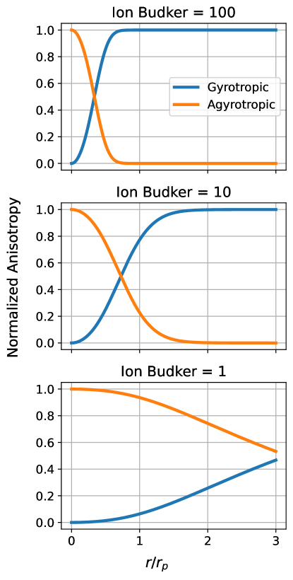
Figure 2 shows the gyrotropic and agyrotropic ion anisotropy profiles predicted by Eqs. 16 for various ion Budker parameters. The model predicts that agyrotropic anisotropy (induced by collisionless compression of ion betatron orbits) is dominant for small Budker parameters, while gyrotropic anisotropy (from collisionless compression of ion cyclotron trajectories) is dominant in the opposite limit. In the intermediate regime, $\mathfrak{B}_{i}=\mathcal{O}(10)$, ion agyrotropy terminates in the vicinity of the pinch radius, which has important consequences for the transport of axial momentum and diamagnetic response of the compressing plasma discussed in the remainder of this work.

In addition to adiabatic compression, agyrotropic anisotropy may be induced non-adiabatically due to collisionless shock heating Gedalin (2022) during fast Z pinch compression. Agyrotropy is induced in collisionless shock heating due to electric field gradients on the scale of the ion inertial length. In addition, radial electric field gradients induced by entropy mode fluctuations Ricci, Rogers, and Dorland (2006) and ensuing kinetic turbulence could also contribute to agyrotropy in ion distributions. Agyrotropic heating is frequently observed in simulations of kinetic plasma turbulence on ion inertial length scales Servidio et al. (2015); Yang et al. (2023). In this connection, note that species inertial length $\delta_{s}=c/\omega_{ps}$ is directly proportional to pinch radius through the species Budker parameter Mahajan (1989); $\mathfrak{B}_{s}=\frac{r_{p}^{2}}{4\lambda_{s}^{2}}$. Finally, strong electric fields can significantly modify particle orbits and drifts, particularly around magnetic O-points Joseph (2021).

Figure 3 presents a visual aid to the discussion of Section III.2, presenting an example of betatron heating and acceleration in a compressing azimuthal magnetic flux. An ion with $P_{z}>0$ is evolved in the model time-dependent $\hat{z}$-directed vector potential $A_{z}=-A_{0}(t)\frac{r^{2}}{2a^{2}}$, with $a=1$ and $A_{0}(t)$ a specified flux compression function. The ion is released from $r=1$ with $v_{r}=0$ and $v_{z}=1$, and the flux factor $A_{0}(t)$ is linearly and slowly varied from an initial value to a final value.

The inductive electric field $E_{z}=-\partial_{t}A_{z}$ does work on the ion, increasing both the radial bounce energy and the axial drift/bounce energy in step (minus $P_{z}^{2}/2m$). Most of the axial oscillation energy is channeled into the axial drift motion, increasing the axial bounce energy in the drifting frame much less than the radial bounce energy, because most of the axial energy in Fig. 3 is composed of the Galillean energy boost $\langle v_{z}\rangle\cdot\delta v_{z}$ from the oscillation-center frame to the lab frame. Thus, betatron heating displays radial/axial temperature anisotropy because the change in radial bounce energy is distinct from the change in axial bounce energy in the drifting frame.

During collisionless adiabatic flux compression of a large Larmor radius Z pinch, mean ion betatron drift changes self-consistently with plasma current and density, and mean radial bounce energy varies so that radial pressure balances the self-magnetic energy $\frac{\mu_{0}}{8\pi}I^{2}$ (Bennett relation). Axial temperature is unconstrained by radial force balance, but is constrained by kinetic equilibrium considerations (which was not appreciated in early Z-pinch studies, see for example the claim in Bennett 1934 that axial temperature is irrelevant to equilibrium Bennett (1934)).

To begin, we present the aforementioned method Suzuki and Shigeyama (2008) to generate a self-consistent kinetic equilibrium using the properties of Hermite polynomials. Consider the ansatz distribution

$$f(A_{z},H)=n_{0}\Big{(}\frac{\beta}{2\pi}\Big{)}^{3/2}\Big{(}\sum_{n=0}^{\infty}g_{n}(A_{z})H_{n}(v_{z})\Big{)}e^{-\beta H}$$

(18)

with $H=\frac{m}{2}(v_{x}^{2}+v_{y}^{2}+v_{z}^{2})+q\varphi$ the energy, $\beta=(k_{B}T)^{-1}$ the inverse temperature, $H_{n}$ the Hermite polynomials, $A_{z}$ the $z$-component of magnetic potential, and $\varphi$ the electric potential. Equation 18 is a kinetic equilibrium with $f=f(P_{z},H)$ provided that

$$\sum_{n=0}^{\infty}(g_{n}^{\prime}(a_{z})H_{n}(v_{z})-g_{n}(a_{z})H_{n}^{\prime}(v_{z}))=0$$

(19)

as found by substitution of Eq. 18 into the kinetic equation. Here the vector potential is written in lower case when it takes on the units of velocity, $a_{z}\equiv qA_{z}/m$, and it is normalized to the thermal speed $v_{t}$. Equation 19 is satisfied if each term of the series balances such that

$$\frac{dg_{n}}{da_{z}}H_{n}=g_{n}\frac{dH_{n}}{dv_{z}}.$$

(20)

Now, the Hermite polynomials are the orthogonal family with the property $H_{n}^{\prime}(x)=2nH_{n-1}(x)$. Substitution of the Hermite property into Eq. 20 shows that the coefficient functions $g_{n}$ must satisfy the recurrence relation

$$g_{n+1}=\frac{1}{2(n+1)}\frac{dg_{n}}{da_{z}}.$$

(21)

Iteratively substituting Eq. 21 into Eq. 18 gives the series

$$f=n_{0}\Big{(}\frac{\beta}{2\pi}\Big{)}^{3/2}\Big{(}\sum_{n=0}^{\infty}\frac{1}{2^{n}n!}\frac{d^{n}g_{0}}{da_{z}^{n}}H_{n}(v_{z})\Big{)}e^{-\beta H}$$

(22)

with $g_{0}=g_{0}(a_{z})$ the first Hermite coefficient. The particle density and current density follow as

	$\displaystyle n_{\alpha}(\varphi,a_{z})$	$\displaystyle=$	$\displaystyle n_{0}g_{0\alpha}(a_{z})e^{-\beta_{\alpha}q_{\alpha}\varphi},$		(23a)
	$\displaystyle j_{z,\alpha}$	$\displaystyle=$	$\displaystyle q_{\alpha}n_{0}v_{t\alpha}\frac{dg_{0,\alpha}}{da_{z}}e^{-\beta_{\alpha}q_{\alpha}\varphi}$		(23b)

because $H_{0,1}(z)=1,2z$ are orthogonal to all other $H_{n}$ over the Gaussian weighting ($e^{-\beta H}$). Equation 22 solves the kinetic equation, and its moments consistently solve the Vlasov-Maxwell system provided it satisfies the nonlinear Poisson equations

	$\displaystyle\nabla^{2}\varphi$	$\displaystyle=$	$\displaystyle\varepsilon_{0}^{-1}\sum_{\alpha}q_{\alpha}n_{0\alpha}g_{0\alpha}(a_{z})e^{-\beta_{\alpha}q_{\alpha}\varphi},$		(24a)
	$\displaystyle\nabla^{2}A_{z}$	$\displaystyle=$	$\displaystyle\mu_{0}\sum_{\alpha}q_{\alpha}n_{0\alpha}v_{t\alpha}\frac{dg_{0\alpha}}{da_{z}}e^{-\beta_{\alpha}q_{\alpha}\varphi}.$		(24b)

Thus, the function $g_{0}=g_{0}(a_{z})$ is a generating function for the equilibrium, determining density, current density, and distribution function in the laboratory frame through its derivatives. Recalling that axial magnetic vector potential is magnetic flux per unit length ($\psi_{\theta}^{\prime}\equiv\int_{0}^{r}B_{\theta}(r^{\prime})dr^{\prime}=-A_{z}$), this means that the generating function and all of its derivatives (the fluid moments) are flux functions. Notably, the toroidal flux function in kinetic tokamak equilibrium can be treated analogously through an azimuthal momentum ($P_{\theta}$) expansion Kaltsas et al. (2024). Intuitively, the generating function of a distribution canonical in the energy is expressed in Hermite series due to the properties of the Weierstrass transform, for which $e^{-\beta H}$ is the kernel Allanson et al. (2016). We now explore a few paradigmatic equilibria in terms of simple generating functions.

The kinetic equilibrium of radially uniform axial velocity is the isothermal Bennett pinch, whose distribution is semi-canonical (namely, a shifted Maxwellian). The function $g_{0}(a_{z})$ is exponential in $a_{z}$,

$$g_{0s}(a_{z})=\exp(2m_{s}\beta_{s}u_{0s}a_{z}).$$

(25)

Repeated differentiation of Eq. 25 and application of the Hermite generating function,

	$\displaystyle\frac{d^{n}g_{0s}}{da_{z}^{n}}$	$\displaystyle=$	$\displaystyle\Big{(}\frac{2u_{0}}{v_{ts}}\Big{)}^{n}g_{0}(a_{z}),$		(26a)
	$\displaystyle\sum_{n=0}^{\infty}H_{n}(v_{z})\frac{u_{0}^{n}}{n!}$	$\displaystyle=$	$\displaystyle\exp(2u_{0}v_{z}-u_{0}^{2}),$		(26b)

arrives at the shifted Maxwellian distribution,

$$f_{s}=n_{0s}\Big{(}\frac{\beta_{s}}{2\pi}\Big{)}^{3/2}e^{-\beta_{s}q_{s}(\varphi-2u_{0s}A_{z})}e^{-\beta_{s}m(v_{x}^{2}+v_{y}^{2}+(v_{z}-u_{0})^{2})/2}.$$

(27)

Both the Bennett pinch (cylindrical) and Harris sheet (Cartesian) are generated by Eq. 25 as they satisfy (under quasineutrality in the center-of-charge frame) the Liouville equation

$$\nabla^{2}A_{z}=-Ke^{2A_{z}},$$

(28)

with $K$ the curvature constant Ceccherini et al. (2005). The cylindrical solution to Eq. 28 is the Bennett pinch’s vector potential, given by

$$A_{z}=-A_{0}\ln(1+(r/r_{p})^{2})$$

(29)

where $r_{p}$ is the characteristic pinch radius and $A_{0}=\frac{\mu_{0}}{4\pi}I_{\infty}$ is the self-magnetic flux per unit length ($I_{\infty}$ is the total current enclosed to infinity). Regarding the generating function, it is useful that the following combination is unity,

$$2q_{s}\beta_{s}u_{0}A_{0}=\frac{\mu_{0}}{4\pi}\frac{N_{s}q_{s}^{2}}{m_{s}}\Big{(}\frac{u_{0}}{v_{ts}}\Big{)}^{2}=1$$

(30)

for each species $s$, where $N_{s}$ is the linear density (particles per unit length) of species $s$. The first factor is the species Budker parameter $\mathfrak{B}_{s}$. For the Bennett pinch, the inverse Budker parameter is the drift Mach number for that species Crews, Meier, and Shumlak (2024),

	$\displaystyle\mathfrak{B}_{s}$	$\displaystyle\equiv$	$\displaystyle\frac{q_{s}^{2}}{4\pi\epsilon_{0}}\frac{N_{s}}{m_{s}c^{2}},$		(31a)
	$\displaystyle\mathfrak{B}_{s}^{-1}$	$\displaystyle=$	$\displaystyle\Big{(}\frac{u_{0}}{v_{ts}}\Big{)}^{2}.$		(31b)

From Eq. 30, it follows from the generating function that the Bennett pinch particle and current densities are given by Meier and Shumlak (2021)

	$\displaystyle n_{s}(r)$	$\displaystyle=$	$\displaystyle\frac{N_{s}}{\pi r_{p}^{2}}(1+(r/r_{p})^{2})^{-2},$		(32a)
	$\displaystyle j_{z}(r)$	$\displaystyle=$	$\displaystyle\frac{I_{\infty}}{\pi r_{p}^{2}}(1+(r/r_{p})^{2})^{-2}.$		(32b)

In the isothermal Bennett kinetic equilibrium, both ions and electrons have uniform flow velocities, so their relative velocity is uniform too. As long as the relative velocity of two species is radially uniform then the magnetic potential will satisfy Eq. 28 and will be of the Bennett form, Eq. 29. The equilibrium has the important property that there is no radial electric field in the center-of-charge frame Gratreau (1978) where $u_{i}=-u_{e}$ (assuming $Z_{i}=1$).

The generator of the next simplest equilibrium is quadratic in the flux, namely $g_{0}=\exp(c_{0}a_{z}+c_{1}a_{z}^{2})$ for constants $c_{0}$, $c_{1}$. This equilibrium consists of a two-temperature bi-Maxwellian distribution with an agyrotropic pressure anisotropy supporting a radially sheared axial flow Del Sarto, Pegoraro, and Califano (2016). Anisotropic collisionless equilibria with sheared flows were explored by Mahajan and Hazeltine Mahajan and Hazeltine (2000), whose discussion we summarize here in the context of the Z pinch.

This sheared anisotropic equilibrium is the simplest kinetic equilibrium displaying the relationship between shear and anisotropy, enabling an understanding of how these two phenomena interact in the collisionless regime, which is relevant to Z pinches approaching fusion conditions. All sheared-flow collisionless kinetic equilibria are “inviscid” because they represent a stationary flow profile, which is a notable property. However, as will be discussed later, the collisionless magnetized dynamics should still be considered highly viscous in the sense that initially out-of-equilibrium flow profiles will quickly find a kinetic equilibrium supporting a steady flow.

Proceeding by direct calculation from an ansatz distribution is the simplest way to show existence of the equilibrium and determine its most fundamental properties. Suppose the distribution function is a two-temperature (bi-)Maxwellian whose first velocity moment $\langle v_{z}\rangle=u_{z}(r)$ is radially sheared (with species subscripts suppressed),

$$f(r,\bm{v})=\frac{\beta_{\perp}}{2\pi}\sqrt{\frac{\beta_{z}}{2\pi}}n(r)e^{-\beta_{\perp}\frac{m}{2}(v_{r}^{2}+v_{\theta}^{2})}e^{-\beta_{z}\frac{m}{2}(v_{z}-u_{z}(r))^{2}}.$$

(33)

Substituting Eq. 33 into the Vlasov equation leads to

$$\partial_{t}f+v_{r}\Big{(}\frac{n^{\prime}}{n}+\beta_{\perp}q\varphi^{\prime}+m\beta_{\perp}u_{z}(r)\omega_{c}\Big{)}f+m\beta_{z}v_{r}(v_{z}-u_{z})A_{rz}f=0$$

(34)

where $\omega_{c}=qB/m$, a shear stress drive term $A_{rz}\equiv u_{z}^{\prime}-\alpha_{rz}\omega_{c}$, and the distribution anisotropy is $\alpha_{rz}\equiv 1-T_{z}/T_{r}$ (for $T_{r}=(k\beta_{\perp})^{-1}$). Taking the first radial moment of Eq. 34 yields

$$\partial_{t}(n\langle v_{r}\rangle)=-n^{\prime}kT_{r}-qn\varphi^{\prime}-qnu_{z}B_{\theta}$$

(35)

giving the equilibrium radial force balance $\nabla p=qn(\bm{E}+\bm{v}\times\bm{B})$ because $\langle v_{r}\rangle=0$. The distribution function supports this force balance in equilibrium (that is, with $\partial_{t}f=0$) if the driver $A_{rz}=0$, namely when the anisotropy and shear profile are related by

$$\frac{du_{z}}{dr}=\alpha_{rz}\omega_{c}.$$

(36)

Having assumed a radially constant anisotropy $\alpha_{rz}$, the axial species velocity is then given by $u_{z}=u_{0}-\alpha_{rz}a_{z}$, meaning that the equilibrium velocity profile is a linear flux function.

The bi-Maxwellian distribution is arrived at from the generating function using the completeness relation for Hermite polynomials Wiener (1988), as the derivatives of the generating function are themselves Hermite polynomials. Applying the completeness relation for the sum $\sum_{n}\frac{1}{n!4^{n}}H_{n}(u_{0}+\alpha_{rz}a_{z})H_{n}(v_{z})$ results in a bi-Maxwellian. The algebra is simpler to proceed as above, and as conducted in Mahajan and Hazeltine Mahajan and Hazeltine (2000), who ultimately find the bi-Maxwellian equilibrium for the sheared Bennett equilibrium (following section) to be

$$f(P_{z},H)=\exp(-\beta(H+u_{0}P_{z}+\gamma P_{z}^{2}/2m))$$

(37)

where $\gamma$ is a constant related to the anisotropy. Equation 37 is a nice closed form result for the distribution function whose sheared flow is a linear flux function. Higher-order dependence of the velocity on the flux function is explored in Section IV.4, but the series appear not to sum cleanly into exponentials as in Eq. 37.

Collisionless kinetic equilibrium of a sheared-flow self-pinched plasma is not necessarily a bi-Maxwellian distribution, which occurs for an isothermal pinch of radially constant $\alpha_{rz}$ temperature anisotropy in which flow velocity is a linear function of magnetic flux. Experimental and numerical simulation dynamics likely display both gyrotropic and agyrotropic anisotropies, due both to flow shear and to the asymmetric responses of cyclotron and betatron trajectories to changes in flux; hence general kinetic equilibria should display both axial and azimuthal temperature gradients. Non-isothermal kinetic equilibria are reserved to a future work.

But even considering the isothermal solutions, velocity need not be a linear flux function. Equilibria can be found as any polynomial function of flux. This section studies more general kinetic equilibria such that the axial velocity is some polynomial of the flux function, and studies the characteristic features of these solutions. First observe that the axial velocity is given by a logarithmic derivative of the generating function,

$$\langle v_{z}\rangle=\frac{1}{g_{0}}\frac{dg_{0}}{da_{z}}=\frac{d\ln g_{0}}{da_{z}}.$$

(39)

Thus, each exponential polynomial $g_{0}(a_{z})$ is associated with a velocity profile as a polynomial in the magnetic potential,

$$g_{0}(a_{z})=\exp\Big{(}\sum_{n=0}^{\infty}\frac{c_{n}}{n+1}a_{z}^{n+1}\Big{)}\implies\langle v_{z}\rangle=\sum_{n=0}^{\infty}c_{n}a_{z}^{n}$$

(40)

where $c_{n}$ are some coefficients. Equation 40 is a formal power series expansion of axial velocity about the pinch axis. With the velocity expressed as such a flux function (Eq. 40), we then seek the Hermite series coefficients to determine the equilibrium distribution function.

Substitution of Eq. 40 into Eq. 22 produces the distribution $f=\widetilde{f}(P_{z})e^{-\beta H}$ by the associated function of $P_{z}$, whose Hermite series coefficients are the derivatives of $g_{0}(a_{z})$. Let

$$h(a_{z})\equiv\sum_{n=0}^{\infty}\frac{c_{n}}{n+1}a_{z}^{n+1}$$

(41)

so that $g_{0}=\exp(h(a_{z}))$. Application of Faà di Bruno’s formula to Eq. 40 yields the Hermite coefficients as

$$\frac{d^{n}g_{0}}{da_{z}^{n}}=e^{h(a_{z})}B_{n}(h^{\prime},\cdots,h^{(n)})$$

(42)

where $B_{n}$ is the n’th complete Bell polynomial Bell (1934). Thus, the semi-canonical distribution function associated with the postulated velocity profile of Eq. 40 is

$$f=e^{-\beta H+h(a_{z})}\sum_{n=0}^{\infty}\frac{1}{2^{n}n!}B_{n}(h^{\prime},\cdots,h^{(n)})H_{n}(v_{z}).$$

(43)

It is intuitive to first consider the forward process, namely viscous damping of sheared flows. To begin, we extend the equilibrium analysis of Mahajan and Hazeltine by considering the evolution of an agryotropic distribution initially out-of-equilibrium, that is, when the equilibrium anisotropy condition $A_{rz}=0$ is not met. Assuming initial radial force balance and introducing a collision operator $C[f]$, Eq. 34 can be written as

$$\frac{\partial f}{\partial t}\Big{|}_{t=t_{0}}=C[f]-m\beta_{z}v_{r}(v_{z}-u_{d})A_{rz}f$$

(48)

instantaneously at the initial time $t=t_{0}$. Given the bi-Maxwellian form of $f$, the collisionless term on the RHS of Eq. 48 may be rewritten as derivatives of $f$, giving

$$\frac{\partial f}{\partial t}\Big{|}_{t=t_{0}}=C[f]+\frac{\partial^{2}}{\partial v_{r}\partial v_{z}}(v_{th,r}^{2}A_{rz}f)$$

(49)

and revealing it to be a diffusive operator, where $v_{th,r}^{2}=kT_{r}/m$ is the radial thermal velocity. The mixed-derivatives term of Eq. 49 satisfies many of the features of a collision operator, such as conservation of particles, energy, and momentum, but drives shear stresses by not conserving the off-diagonal pressure tensor components $\Pi_{rz}=\int v_{r}v_{z}fd\bm{v}$.

Adopting a simple collision model such as the Lenard-Bernstein form shows the mixed derivatives to introduce off-diagonal terms to the velocity space diffusion matrix. The Fokker-Planck equation then has the paradigmatic form

	$\displaystyle\frac{df}{dt}$	$\displaystyle=$	$\displaystyle-\nu\nabla_{v}\cdot(\bm{v}f)+v_{t}^{2}\nabla_{v}\cdot(\mathcal{D}\nabla_{v}f),$		(50a)
	$\displaystyle\mathcal{D}$	$\displaystyle=$	$\displaystyle\begin{bmatrix}\nu&A_{rz}/2\\ A_{rz}/2&\nu\end{bmatrix}$		(50b)

where $\nu$ is the relaxation rate and $A_{rz}$ the shear stress drive frequency. The off-diagonal terms produce shearing in the velocity space (demonstrated in Fig. 5) as they are symmetric.

References

- Bennett (1934) W. H. Bennett, “Magnetically self-focussing streams,” Phys. Rev. 45, 890–897 (1934).
- Tonks (1937) L. Tonks, “Theory and phenomena of high current densities in low pressure arcs,” Transactions of The Electrochemical Society 72, 167 (1937).
- Artsimovich (1962) L. A. Artsimovich, “Controlled Nuclear Fusion Research, September 1961: Review of experimental results,” Nuclear Fusion, Suppl. (1962).
- Bostick (1977) W. H. Bostick, “The pinch effect revisited,” International Journal of Fusion Energy 1, 1–55 (1977).
- Lawson (1958) J. D. Lawson, “Perveance and the Bennett Pinch Relation in Partially-Neutralized Electron Beams,” Journal of Electronics and Control 5, 146–151 (1958), https://doi.org/10.1080/00207215808953898 .
- Budker (1956) G. I. Budker, “Relativistic stabilized electron beam,” The Soviet Journal of Atomic Energy 1, 673–686 (1956).
- Linhart (1959) J. G. Linhart, “Accelerated Self-Constricted Electron Streams in Plasma,” Proceedings of the Royal Society of London. Series A, Mathematical and Physical Sciences 249, 318–334 (1959).
- Alfvén (1939) H. Alfvén, “On the Motion of Cosmic Rays in Interstellar Space,” Phys. Rev. 55, 425–429 (1939).
- Lawson (1959) J. D. Lawson, “On the classification of electron streams,” Journal of Nuclear Energy. Part C, Plasma Physics, Accelerators, Thermonuclear Research 1, 31 (1959).
- Crews, Meier, and Shumlak (2024) D. W. Crews, E. T. Meier, and U. Shumlak, “Z Pinch Kinetics I - A Particle Perspective: Transitional Magnetization and Cyclotron and Betatron Orbits,” In preparation (2024).
- Arnold (2013) V. I. Arnold, Mathematical Methods of Classical Mechanics, Graduate Texts in Mathematics (Springer New York, 2013).
- Finkelstein and Sturrock (1959) D. Finkelstein and P. A. Sturrock, “Stability of relativistic self-focusing streams,” in Plasma Physics, Ed. J. E. Drummond (Dover, 1959).
- Bennett (1955) W. H. Bennett, “Self-focusing streams,” Phys. Rev. 98, 1584–1593 (1955).
- Haines (2001) M. G. Haines, “Kinetic effects in z pinches,” Laser and Particle Beams 19, 345–353 (2001).
- Santos et al. (2018) J. J. Santos, M. Bailly-Grandvaux, M. Ehret, A. V. Arefiev, D. Batani, F. N. Beg, A. Calisti, S. Ferri, R. Florido, P. Forestier-Colleoni, S. Fujioka, M. A. Gigosos, L. Giuffrida, L. Gremillet, J. J. Honrubia, S. Kojima, P. Korneev, K. F. F. Law, J.-R. Marquès, A. Morace, C. Mossé, O. Peyrusse, S. Rose, M. Roth, S. Sakata, G. Schaumann, F. Suzuki-Vidal, V. T. Tikhonchuk, T. Toncian, N. Woolsey, and Z. Zhang, “Laser-driven strong magnetostatic fields with applications to charged beam transport and magnetized high energy-density physics,” Physics of Plasmas 25, 056705 (2018), https://pubs.aip.org/aip/pop/article-pdf/doi/10.1063/1.5018735/14700567/056705_1_online.pdf .
- Arefiev et al. (2024) A. Arefiev, I.-L. Yeh, K. Tangtartharakul, and L. Willingale, “Electron energy gain due to a laser frequency modulation experienced by electron during betatron motion,” Physics of Plasmas 31, 023106 (2024), https://pubs.aip.org/aip/pop/article-pdf/doi/10.1063/5.0190559/19725041/023106_1_5.0190559.pdf .
- Vikhrev and Korolev (2007) V. V. Vikhrev and V. D. Korolev, “Neutron generation from Z-pinches,” Plasma Physics Reports 33, 356–380 (2007).
- Goyon et al. (2024) C. Goyon, S. C. Bott-Suzuki, A. E. Youmans, J. T. Banasek, L. A. Morton, B. Levitt, J. R. Barhydt, K. D. Morgan, C. Liekhus-Schmaltz, W. C. Young, D. P. Higginson, A. C. Hossack, E. T. Meier, B. A. Nelson, M. Quinley, A. Taylor, P. Tsai, N. van Rossum, A. Shah, A. D. Stepanov, D. A. Sutherland, T. R. Weber, U. Shumlak, and H. S. McLean, “Plasma pressure profiles in a sheared-flow-stabilized Z-pinch,” Physics of Plasmas 31, 072503 (2024), https://pubs.aip.org/aip/pop/article-pdf/doi/10.1063/5.0209351/20027284/072503_1_5.0209351.pdf .
- Mitrani et al. (2021) J. M. Mitrani, J. A. Brown, B. L. Goldblum, T. A. Laplace, E. L. Claveau, Z. T. Draper, E. G. Forbes, R. P. Golingo, H. S. McLean, B. A. Nelson, U. Shumlak, A. Stepanov, T. R. Weber, Y. Zhang, and D. P. Higginson, “Thermonuclear neutron emission from a sheared-flow stabilized Z-pinch,” Physics of Plasmas 28, 112509 (2021), https://pubs.aip.org/aip/pop/article-pdf/doi/10.1063/5.0066257/13408570/112509_1_online.pdf .
- Kotelnikov (2020) I. Kotelnikov, “On the structure of the boundary layer in a Beklemishev diamagnetic bubble,” Plasma Physics and Controlled Fusion 62, 075002 (2020).
- Timofeev, Kurshakov, and Berendeev (2024) I. V. Timofeev, V. A. Kurshakov, and E. A. Berendeev, “Formation of cylindrical plasma equilibria with ,” Physics of Plasmas 31, 082512 (2024), https://pubs.aip.org/aip/pop/article-pdf/doi/10.1063/5.0216073/20127415/082512_1_5.0216073.pdf .
- Braginskii (1965) S. I. Braginskii, “Transport processes in a plasma,” in Reviews of Plasma Physics, Vol. 1 (Consulants Bureau, New York, 1965).
- Du et al. (2020) S. Du, G. P. Zank, X. Li, and F. Guo, “Energy dissipation and entropy in collisionless plasma,” Phys. Rev. E 101, 033208 (2020).
- Bandyopadhyay et al. (2023) R. Bandyopadhyay, Y. Yang, W. H. Matthaeus, T. N. Parashar, V. Roytershteyn, A. Chasapis, D. J. Gershman, B. L. Giles, and J. L. Burch, “Collisional-like dissipation in collisionless plasmas,” Physics of Plasmas 30, 080702 (2023), https://pubs.aip.org/aip/pop/article-pdf/doi/10.1063/5.0146986/18086698/080702_1_5.0146986.pdf .
- Del Sarto, Pegoraro, and Califano (2016) D. Del Sarto, F. Pegoraro, and F. Califano, “Pressure anisotropy and small spatial scales induced by velocity shear,” Phys. Rev. E 93, 053203 (2016).
- Del Sarto and Pegoraro (2017) D. Del Sarto and F. Pegoraro, “Shear-induced pressure anisotropization and correlation with fluid vorticity in a low collisionality plasma,” Monthly Notices of the Royal Astronomical Society 475, 181–192 (2017), https://academic.oup.com/mnras/article-pdf/475/1/181/23388297/stx3083.pdf .
- Yang et al. (2017) Y. Yang, W. H. Matthaeus, T. N. Parashar, C. C. Haggerty, V. Roytershteyn, W. Daughton, M. Wan, Y. Shi, and S. Chen, “Energy transfer, pressure tensor, and heating of kinetic plasma,” Physics of Plasmas 24, 072306 (2017), https://pubs.aip.org/aip/pop/article-pdf/doi/10.1063/1.4990421/15999836/072306_1_online.pdf .
- Kaufman (1960) A. N. Kaufman, “Plasma Viscosity in a Magnetic Field,” Physics of Fluids (1960), 10.1063/1.1706096.
- Hellinger, Petr et al. (2024) Hellinger, Petr, Verdini, Andrea, Montagud-Camps, Victor, Franci, Luca, Papini, Emanuele, Matteini, Lorenzo, and Landi, Simone, “Anisotropy of plasma turbulence at ion scales: Hall and pressure–strain effects,” A&A 684, A120 (2024).
- Bandyopadhyay et al. (2020) R. Bandyopadhyay, W. H. Matthaeus, T. N. Parashar, Y. Yang, A. Chasapis, B. L. Giles, D. J. Gershman, C. J. Pollock, C. T. Russell, R. J. Strangeway, R. B. Torbert, T. E. Moore, and J. L. Burch, “Statistics of Kinetic Dissipation in the Earth’s Magnetosheath: MMS Observations,” Phys. Rev. Lett. 124, 255101 (2020).
- Pezzi et al. (2019) O. Pezzi, Y. Yang, F. Valentini, S. Servidio, A. Chasapis, W. H. Matthaeus, and P. Veltri, “Energy conversion in turbulent weakly collisional plasmas: Eulerian hybrid Vlasov-Maxwell simulations,” Physics of Plasmas 26, 072301 (2019), https://pubs.aip.org/aip/pop/article-pdf/doi/10.1063/1.5100125/13820638/072301_1_online.pdf .
- Cassak and Barbhuiya (2022) P. A. Cassak and M. H. Barbhuiya, “Pressure–strain interaction. I. On compression, deformation, and implications for Pi-D,” Physics of Plasmas 29, 122306 (2022), https://pubs.aip.org/aip/pop/article-pdf/doi/10.1063/5.0125248/19799503/122306_1_online.pdf .
- Cassak, Barbhuiya, and Weldon (2022) P. A. Cassak, M. H. Barbhuiya, and H. A. Weldon, “Pressure–strain interaction. II. Decomposition in magnetic field-aligned coordinates,” Physics of Plasmas 29, 122307 (2022), https://pubs.aip.org/aip/pop/article-pdf/doi/10.1063/5.0125252/19799488/122307_1_online.pdf .
- Barbhuiya and Cassak (2022) M. H. Barbhuiya and P. A. Cassak, “Pressure–strain interaction. III. Particle-in-cell simulations of magnetic reconnection,” Physics of Plasmas 29, 122308 (2022), https://pubs.aip.org/aip/pop/article-pdf/doi/10.1063/5.0125256/19799538/122308_1_online.pdf .
- Conley et al. (2024) S. A. Conley, J. Juno, J. M. TenBarge, M. H. Barbhuiya, P. A. Cassak, G. G. Howes, and E. Lichko, “The kinetic analogue of the pressure-strain interaction,” (2024), arXiv:2408.06508 [physics.plasm-ph] .
- Shumlak (2020) U. Shumlak, “Z-pinch fusion,” Journal of Applied Physics 127, 200901 (2020), https://pubs.aip.org/aip/jap/article-pdf/doi/10.1063/5.0004228/19782092/200901_1_online.pdf .
- Ryutov, Derzon, and Matzen (2000) D. D. Ryutov, M. S. Derzon, and M. K. Matzen, “The physics of fast pinches,” Rev. Mod. Phys. 72, 167–223 (2000).
- Morozov and Solov’ev (1980) A. I. Morozov and L. S. Solov’ev, “Steady-state plasma flow in a magnetic field,” in Reviews of Plasma Physics, edited by M. A. Leontovich (Springer US, Boston, MA, 1980) pp. 1–103.
- Turchi and Shumlak (2023) P. J. Turchi and U. Shumlak, “Some Considerations of a Flow-Stabilized Z-Pinch for Megagauss Fusion,” IEEE Transactions on Plasma Science 51, 3679–3687 (2023).
- Crews et al. (2024) D. W. Crews, I. A. M. Datta, E. T. Meier, and U. Shumlak, “The Kadomtsev Pinch Revisited for Sheared-Flow-Stabilized Z-Pinch Modeling,” IEEE Transactions on Plasma Science , 1–13 (2024).
- Hunana et al. (2022) P. Hunana, T. Passot, E. Khomenko, D. Martínez-Gómez, M. Collados, A. Tenerani, G. P. Zank, Y. Maneva, M. L. Goldstein, and G. M. Webb, “Generalized Fluid Models of the Braginskii Type,” The Astrophysical Journal Supplement Series 260, 26 (2022).
- Meier and Shumlak (2021) E. T. Meier and U. Shumlak, “Development of five-moment two-fluid modeling for Z-pinch physics,” Physics of Plasmas 28, 092512 (2021), https://pubs.aip.org/aip/pop/article-pdf/doi/10.1063/5.0058420/13420598/092512_1_online.pdf .
- Ryutov (2015) D. D. Ryutov, “Characterizing the Plasmas of Dense -Pinches,” IEEE Transactions on Plasma Science 43, 2363–2384 (2015).
- Shumlak, Meier, and Levitt (2024) U. Shumlak, E. T. Meier, and B. J. Levitt, “Fusion Gain and Triple Product for the Sheared-Flow-Stabilized Z Pinch,” Fusion Science and Technology 80, 1–16 (2024), https://doi.org/10.1080/15361055.2023.2198049 .
- Bott, Cowley, and Schekochihin (2024) A. F. A. Bott, S. C. Cowley, and A. A. Schekochihin, “Kinetic stability of Chapman–Enskog plasmas,” Journal of Plasma Physics 90, 975900207 (2024).
- Braginskii (1958) S. I. Braginskii, “Transport processes in a plasma,” Reviews of Plasma Physics 1, 358–369 (1958).
- Chew, Goldberger, and Low (1956) G. F. Chew, M. L. Goldberger, and F. E. Low, “The Boltzmann Equation and the One-Fluid Hydromagnetic Equations in the Absence of Particle Collisions,” Proceedings of the Royal Society of London. Series A, Mathematical and Physical Sciences 236, 112–118 (1956).
- Sonnerup (1971) B. U. O. Sonnerup, “Adiabatic particle orbits in a magnetic null sheet,” Journal of Geophysical Research (1896-1977) 76, 8211–8222 (1971), https://agupubs.onlinelibrary.wiley.com/doi/pdf/10.1029/JA076i034p08211 .
- Janicke (1975) L. Janicke, “Adiabatische invarianz im mittel / adiabatic invariance in the average,” Zeitschrift für Naturforschung A 30, 421–430 (1975).
- Cary, Escande, and Tennyson (1986) J. R. Cary, D. F. Escande, and J. L. Tennyson, “Adiabatic-invariant change due to separatrix crossing,” Phys. Rev. A 34, 4256–4275 (1986).
- Büchner and Zelenyi (1989) J. Büchner and L. M. Zelenyi, “Regular and chaotic charged particle motion in magnetotaillike field reversals: 1. Basic theory of trapped motion,” Journal of Geophysical Research: Space Physics 94, 11821–11842 (1989), https://agupubs.onlinelibrary.wiley.com/doi/pdf/10.1029/JA094iA09p11821 .
- Ochs and Fisch (2018) I. E. Ochs and N. J. Fisch, “Anisotropy-driven collisional separation of impurities in magnetized compressing and expanding cylindrical plasmas,” Physics of Plasmas 25, 122306 (2018), https://pubs.aip.org/aip/pop/article-pdf/doi/10.1063/1.5055568/15779257/122306_1_online.pdf .
- Gedalin (2022) M. Gedalin, “Combining Rankine–Hugoniot relations, ion dynamics in the shock front, and the cross-shock potential,” Physics of Plasmas 29, 112904 (2022), https://pubs.aip.org/aip/pop/article-pdf/doi/10.1063/5.0120578/16630179/112904_1_online.pdf .
- Ricci, Rogers, and Dorland (2006) P. Ricci, B. N. Rogers, and W. Dorland, “Small-Scale Turbulence in a Closed-Field-Line Geometry,” Phys. Rev. Lett. 97, 245001 (2006).
- Servidio et al. (2015) S. Servidio, F. Valentini, D. Perrone, A. Greco, F. Califano, W. H. Matthaeus, and P. Veltri, “A kinetic model of plasma turbulence,” Journal of Plasma Physics 81, 325810107 (2015).
- Yang et al. (2023) Y. Yang, F. Pecora, W. H. Matthaeus, S. Roy, M. E. Cuesta, A. Chasapis, T. Parashar, R. Bandyopadhyay, D. J. Gershman, B. L. Giles, and J. L. Burch, “Quantifying the Agyrotropy of Proton and Electron Heating in Turbulent Plasmas,” The Astrophysical Journal 944, 148 (2023).
- Mahajan (1989) S. M. Mahajan, “Exact and almost exact solutions to the Vlasov–Maxwell system,” Physics of Fluids B: Plasma Physics 1, 43–54 (1989).
- Joseph (2021) I. Joseph, “Guiding center and gyrokinetic orbit theory for large electric field gradients and strong shear flows,” Physics of Plasmas 28, 042102 (2021), https://pubs.aip.org/aip/pop/article-pdf/doi/10.1063/5.0037889/16004149/042102_1_online.pdf .
- Helander and Mackenbach (2024) P. Helander and R. J. J. Mackenbach, “Available energy of plasmas with small fluctuations,” Journal of Plasma Physics 90, 905900401 (2024).
- Livadiotis and McComas (2013) G. Livadiotis and D. J. McComas, “Understanding kappa distributions: A toolbox for space science and astrophysics,” Space Science Reviews 175, 183–214 (2013).
- Livadiotis and McComas (2024) G. Livadiotis and D. J. McComas, “Universality of kappa distributions,” Europhysics Letters 146, 41003 (2024).
- Suzuki and Shigeyama (2008) A. Suzuki and T. Shigeyama, “A novel method to construct stationary solutions of the Vlasov–Maxwell system,” Physics of Plasmas 15 (2008).
- Channell (1976) P. J. Channell, “Exact Vlasov–Maxwell equilibria with sheared magnetic fields,” The Physics of Fluids 19, 1541–1545 (1976), https://pubs.aip.org/aip/pfl/article-pdf/19/10/1541/12443456/1541_1_online.pdf .
- Allanson et al. (2016) O. Allanson, T. Neukirch, S. Troscheit, and F. Wilson, “From one-dimensional fields to Vlasov equilibria: theory and application of Hermite polynomials,” Journal of Plasma Physics 82, 905820306 (2016).
- Kaltsas et al. (2024) D. A. Kaltsas, A. Kuiroukidis, P. J. Morrison, and G. N. Throumoulopoulos, “Axisymmetric hybrid Vlasov equilibria with applications to tokamak plasmas,” Plasma Physics and Controlled Fusion 66, 065016 (2024).
- Ceccherini et al. (2005) F. Ceccherini, C. Montagna, F. Pegoraro, and G. Cicogna, “Two-dimensional Harris–Liouville plasma kinetic equilibria,” Physics of Plasmas 12, 052506 (2005), https://pubs.aip.org/aip/pop/article-pdf/doi/10.1063/1.1899083/13506459/052506_1_online.pdf .
- Gratreau (1978) P. Gratreau, “Generalized Bennett equilibria and particle orbit analysis of plasma columns carrying ultra-high currents,” The Physics of Fluids 21, 1302–1311 (1978), https://pubs.aip.org/aip/pfl/article-pdf/21/8/1302/12259969/1302_1_online.pdf .
- Mahajan and Hazeltine (2000) S. M. Mahajan and R. D. Hazeltine, “Sheared-flow generalization of the Harris sheet,” Physics of Plasmas 7, 1287–1293 (2000), https://pubs.aip.org/aip/pop/article-pdf/7/4/1287/19322230/1287_1_online.pdf .
- Wiener (1988) N. Wiener, The Fourier integral and certain of its applications (CUP Archive, 1988).
- Channon and Coppins (2001) S. W. Channon and M. Coppins, “Z-pinch Vlasov-fluid equilibria including sheared-axial flow,” Journal of Plasma Physics 66, 337–347 (2001).
- Bell (1934) E. T. Bell, “Exponential Polynomials,” Annals of Mathematics 35, 258–277 (1934).
- Dattoli et al. (1994) G. Dattoli, C. Chiccoli, S. Lorenzutta, G. Maino, and A. Torre, “Theory of generalized Hermite polynomials,” Computers and Mathematics with Applications 28, 71–83 (1994).
- Torre (2012) A. Torre, “Airy polynomials, three-variable Hermite polynomials and the paraxial wave equation,” Journal of Optics 14, 045704 (2012).
- Malara et al. (2022) F. Malara, A. Settino, D. Perrone, O. Pezzi, G. Guzzi, and F. Valentini, “Exact shearing flow magnetized hybrid kinetic equilibria with inhomogeneous temperature,” The Astrophysical Journal 941, 201 (2022).
- Gedalin (2015) M. Gedalin, “Collisionless relaxation of non-gyrotropic downstream ion distributions: dependence on shock parameters,” Journal of Plasma Physics 81, 905810603 (2015).
- Velikhov (1964) E. P. Velikhov, “A note on plasma rotation,” Journal of Nuclear Energy. Part C, Plasma Physics, Accelerators, Thermonuclear Research 6, 203 (1964).
- Haines (1965) M. G. Haines, “On the origin of rotation in magnetically confined plasmas,” Advances in Physics 14, 167–211 (1965), https://doi.org/10.1080/00018736500101031 .
- Channon, Coppins, and Arber (1999) S. W. Channon, M. Coppins, and T. D. Arber, “One-dimensional hybrid simulations of the imploding large Larmor radius Z pinch,” Physics of Plasmas 6, 3890–3897 (1999), https://pubs.aip.org/aip/pop/article-pdf/6/10/3890/19159658/3890_1_online.pdf .
- Channon et al. (2004) S. Channon, I. Mitchell, E. Wyndam, M. Favre, and H. Chuaquai, “Sheared Flow Generation in Imploding Vlasov-Fluid Plasmas,” Physica Scripta 69, 30 (2004).
- Del Sarto, Pegoraro, and Tenerani (2017) D. Del Sarto, F. Pegoraro, and A. Tenerani, “‘Magneto-elastic’ waves in an anisotropic magnetised plasma,” Plasma Physics and Controlled Fusion 59, 045002 (2017).
- Fetsch and Fisch (2024) H. Fetsch and N. J. Fisch, “Enhancement to fusion reactivity in sheared flows,” (2024), arXiv:2410.03590 [physics.plasm-ph] .
- Haines (2011) M. G. Haines, “A review of the dense Z-pinch,” Plasma Physics and Controlled Fusion 53, 093001 (2011).
- Miller and Shumlak (2016) S. T. Miller and U. Shumlak, “A multi-species 13-moment model for moderately collisional plasmas,” Physics of Plasmas 23, 082303 (2016), https://pubs.aip.org/aip/pop/article-pdf/doi/10.1063/1.4960041/16032187/082303_1_online.pdf .
- Lucibello (2024a) P. Lucibello, “Z-Pinch Stabilization by a Frozen-In Axial Magnetic Flux,” IEEE Transactions on Plasma Science 52, 310–318 (2024a).
- Vogman, Shumlak, and Colella (2018) G. Vogman, U. Shumlak, and P. Colella, “Conservative fourth-order finite-volume Vlasov–Poisson solver for axisymmetric plasmas in cylindrical phase space coordinates,” Journal of Computational Physics 373, 877–899 (2018).
- Shumlak and Hartman (1995) U. Shumlak and C. W. Hartman, “Sheared Flow Stabilization of the Kink Mode in Pinches,” Phys. Rev. Lett. 75, 3285–3288 (1995).
- Spies (1988) G. O. Spies, “Visco-resistive stabilization of kinks with short wavelengths along an elliptic magnetic stagnation line,” Plasma Physics and Controlled Fusion 30, 1025 (1988).
- Lucibello (2024b) P. Lucibello, “On axial current induction and stability of a pinch,” IEEE Transactions on Plasma Science , 1–15 (2024b).
- Bai et al. (2023) X. Bai, Y. Liu, G. Hao, G. Dong, N. Zhang, and S. Wang, “A new mechanism for internal kink stabilization by plasma flow and anisotropic thermal transport,” Nuclear Fusion 64, 014001 (2023).
- Guillevic et al. (2023) A. Guillevic, M. Lesur, X. Garbet, P. Diamond, G. Lo-Cascio, Y. Kosuga, E. Gravier, D. Mandal, A. Ghizzo, and T. Réveillé, “Particle dynamics in a turbulent electric field,” Physics of Plasmas 30, 052301 (2023), https://pubs.aip.org/aip/pop/article-pdf/doi/10.1063/5.0135918/17177512/052301_1_5.0135918.pdf .
- Pierce and Kim (2023) C. M. Pierce and Y.-K. Kim, “Kernel density estimators for axisymmetric particle beams,” Instruments 7 (2023), 10.3390/instruments7040044.
- Trubnikov (1992) B. A. Trubnikov, “A new hypothesis of cosmic ray generation in plasma pinches,” IEEE Transactions on Plasma Science 20, 898–904 (1992).
- Srinivasan and Hakim (2018) B. Srinivasan and A. Hakim, “Role of electron inertia and electron/ion finite Larmor radius effects in low-beta, magneto-Rayleigh-Taylor instability,” Physics of Plasmas 25, 092108 (2018), https://pubs.aip.org/aip/pop/article-pdf/doi/10.1063/1.5046098/15884196/092108_1_online.pdf .
- Vold et al. (2018) E. Vold, G. Kagan, A. N. Simakov, K. Molvig, and L. Yin, “Self-similar solutions for multi-species plasma mixing by gradient driven transport,” Plasma Physics and Controlled Fusion 60, 054010 (2018).