YITP-20-102
Symmetry enhancement in a two-logarithm matrix model
and the canonical tensor model

Quantum gravity is one of the serious fundamental problems in theoretical physics. This problem originates from the fact that it is difficult to apply the standard quantum field theoretical method to the quantization of general relativity²²2However, see for example [1] for a sophisticated quantum field theoretical approach.. Various approaches have been proposed, and some of them argue that macroscopic spacetimes and general relativity are emergent phenomena from collective dynamics of some fundamental degrees of freedom [2, 3, 4, 5].

The tensor model may be regarded as one of such approaches [6, 7, 8, 9]. It was introduced as an extension of the matrix model, which successfully describes the two-dimensional quantum gravity [10], with the hope to extend the success to higher dimensions. However, the tensor model does not seem to generate macroscopic spacetimes but is rather dominated by singular objects like branched polymers³³3See [11, 12] for the proof in the large $N$ limit in the colored tensor model.. Therefore, it seems difficult to regard the tensor model as quantum gravity for dimensions higher than two.

The tensor model above is in the context of Euclidean simplicial quantum gravity. In fact, simplicial quantum gravity is more successful in the Lorentzian context: It has been shown that the causal dynamical triangulation, the Lorentzian version, successfully generates macroscopic spacetimes [13], while the dynamical triangulation, the Euclidean version, does not. Prompted by the success, the present author has formulated a tensor model in the Hamilton formalism, which we call the canonical tensor model (CTM) [14, 15]. CTM is a first-class constrained system having an analogous structure as the Arnowitt-Deser-Misner (ADM) formalism of general relativity. The canonical quantization of CTM is straightforward [16], and the physical state condition can exactly be solved by a wave function [17].

The wave function is represented by a multiple integral of an integrand which has an argument of a real symmetric tensor $P_{abc}\ (a,b,c=1,\ldots,N)$ [17] (See Appendix A for a minimal introduction.). It has been argued in general contexts and has been shown for some simple cases that the wave function has peaks at Lie-group symmetric configurations (namely, $P_{abc}=g_{a}^{a^{\prime}}g_{b}^{b^{\prime}}g_{b}^{b^{\prime}}P_{a^{\prime}b^{\prime}c^{\prime}},\ g\in G$) for various Lie-group representations $G$ [18, 19]. This phenomenon, which may be called symmetry emergence from quantum coherence, would be interesting from the perspective of spacetime emergence, since spacetimes could potentially be realized as gauge orbits of Lie group representations⁴⁴4In fact, the peaks of the wave function of CTM form a ridge along configurations invariant under a Lorentzian Lie group $SO(n,1)$ rather than a Euclidean Lie group [19]. However, we need more thorough knowledge of the phenomenon to argue for spacetime emergence, including large $N$ limits, in which continuum spacetimes are expected to appear.

In the previous works [20, 21, 22, 23], we studied the wave function in the negative cosmological constant case through a matrix model with non-pairwise index contractions. However, real interesting properties of CTM are expected to appear in the positive cosmological constant case, since the symmetry emergence phenomenon mentioned above is much more evident in the positive case than the negative [19]. Here the Monte Carlo simulations performed in the previous works [21, 22, 23] cannot easily be applied, because the quantity to be computed for the positive case suffers from the notorious sign problem of Monte Carlo simulations.

In this paper, we consider a matrix version of the wave function of CTM by replacing the tensor argument $P_{abc}$ with a matrix $M_{ab}$. This of course is not an approximation to the wave function, but its similarity makes the correspondence of the parameters and the interpretations between the matrix and the tensor versions possible. An advantage of the matrix version is that it can be computed even for the positive cosmological constant case, as we will see. As will be explained in Section 2, the matrix model we consider comes from the absolute square norm of the matrix version of the wave function, and is given by a one-matrix model of a real symmetric matrix $M_{ab}\ (a,b=1,2,\cdots,N)$ with a partition function defined by

$\displaystyle Z=\int_{\mathbb{R}^{\#M}}\prod_{a,b=1\atop a\leq b}^{N}dM_{ab}\,e^{-S(M)},$

(1)

where $\#M=N(N+1)/2$, namely, the number of independents components of $M_{ab}$, and

$\displaystyle S(M):={\rm Tr}\left[\frac{R}{2}\log(k_{1}+ik_{2}-iM)+\frac{R}{2}\log(k_{1}-ik_{2}+iM)+\alpha M^{2}\right]$

(2)

with positive parameters, $R,k_{1},k_{2},\alpha$. The parameters have a redundancy under the rescaling of $M_{ab}$, and $\alpha=1$ may be taken in the following sections.

A similar matrix model with two logarithmic functions has been considered in a different context in [24] with a difference of the last term in (2).

As explained in Appendix A, (62) gives the wave function corresponding to the exactly solved physical state [17] of CTM mentioned in Section 1. We consider an analogous wave function which is obtained by replacing $P_{abc}$ with $M_{ab}$:

$\displaystyle\begin{split}&\Psi(M):=\langle M|\Psi\rangle=\varphi(M)^{R},\\ &\varphi(M):=\int_{\mathbb{R}^{N}}\prod_{a=1}^{N}d\phi_{a}\,e^{iM_{ab}\phi_{a}\phi_{b}-(k_{1}+ik_{2})\phi_{a}\phi_{a}},\end{split}$

(3)

where the repeated indices are assumed to be summed over. Here the integration region is the whole $N$-dimensional real space, $M_{ab}$ is a real symmetric matrix, and $k_{1},k_{2},R$ are assumed to be positive⁵⁵5The sign of $k_{2}$ can always be chosen positive by the replacement $M\rightarrow-M$.. The part containing $k_{1},k_{2}$ of the integrand is an analogue to the Airy function in (62). If $k_{1}$ dominates, the part becomes a damping function corresponding to the negative cosmological constant case in CTM, but, if $k_{2}$ dominates, the part becomes oscillatory corresponding to the positive cosmological constant case. As explained in Section 1, since we are mainly interested in the positive cosmological constant case, our main focus is on the case with finite $k_{2}$ and small $k_{1}$. More precisely, $\tilde{k}_{1}=k_{1}/\sqrt{N}\ll 1$ (which will appear later) is implicitly assumed throughout this paper.

Let us consider the following observable for the state,

$\displaystyle\langle\Psi|e^{-\alpha\hat{M}^{2}}|\Psi\rangle=\int_{{\mathbb{R}}^{\#M}}\prod_{a,b=1\atop a\leq b}^{N}dM_{ab}\left|\Psi(M)\right|^{2}\,e^{-\alpha M^{2}},$

(4)

where $\alpha$ is a positive parameter, $M^{2}:=M_{ab}M_{ab}$, and the integration is over the whole $\#M$-dimensional real space. By performing the gaussian integration over $\phi_{a}$ in (3) and putting the result into (4), we obtain

$\displaystyle\langle\Psi|e^{-\alpha\hat{M}^{2}}|\Psi\rangle=const.\,Z,$

(5)

where $Z$ is given in (1), and the overall constant is irrelevant.

It would be instructive to cast the same system into a different expression. Let us assume $R$ is an integer. Then the $R$-th power of the wave function (3) can be replaced by introducing $R$ replicas of $\phi_{a}$:

$\displaystyle\Psi(M)=\varphi(M)^{R}=\int_{\mathbb{R}^{NR}}\prod_{a,l=1}^{N,R}d\phi_{a}^{l}\,e^{\sum_{l=1}^{R}iM_{ab}\phi_{a}^{l}\phi_{b}^{l}-(k_{1}+ik_{2})\phi_{a}^{l}\phi_{a}^{l}}.$

(6)

Considering the same replacement for the complex conjugate $\Psi^{*}(M)$ with variable $\tilde{\phi}_{a}^{l}$, putting them into (4), and integrating over $M$, we obtain

$\displaystyle Z=const.\int\prod_{a,l=1}^{N,R}d\phi_{a}^{l}d\tilde{\phi}_{a}^{l}\ e^{-S_{\phi}},$

(7)

where

$\displaystyle S_{\phi}:=\frac{1}{4\alpha}\left(\hbox{Tr}\left[\phi\phi^{t}\phi\phi^{t}\right]+\hbox{Tr}\left[\tilde{\phi}\tilde{\phi}^{t}\tilde{\phi}\tilde{\phi}^{t}\right]-2\hbox{Tr}\left[\phi\phi^{t}\tilde{\phi}\tilde{\phi}^{t}\right]\right)+(k_{1}+ik_{2})\hbox{Tr}\left[\phi\phi^{t}\right]+(k_{1}-ik_{2})\hbox{Tr}\left[\tilde{\phi}\tilde{\phi}^{t}\right],$

(8)

where $(\phi\phi^{t})_{ab}:=\sum_{l=1}^{R}\phi_{a}^{l}\phi_{b}^{l}$. This may be regarded as a special choice of the parameters of the 8-vertex matrix model presented in [25]. This can also be regarded as a usual matrix analogue to the matrix model with non-pairwise index contractions which has been analyzed in [20, 21, 22, 23] in the context of CTM.

In this section, we give an intuitive picture of the dynamics of the matrix model (1) by regarding it as an aligned Coulomb gas system. A solid treatment of the matrix model by the Schwinger-Dyson equation will be discussed in Section 4.

The partition function of the matrix model can be rewritten by using its invariance under the $SO(N)$ transformation $M^{\prime}=LML^{t},\ L\in SO(N)$. Denoting the eigenvalues of $M$ by $\lambda_{a}\ (a=1,2,\ldots,N)$, which are all real, one obtains

	$\displaystyle Z$	$\displaystyle=const.\int_{\mathbb{R}^{N}}\prod_{a=1}^{N}d\lambda_{a}\prod_{a,b=1\atop a<b}^{N}|\lambda_{a}-\lambda_{b}|\ e^{-\sum_{a=1}^{N}S(\lambda_{a})}$		(9)
		$\displaystyle=const.\int_{\mathbb{R}^{N}}\prod_{a=1}^{N}d\lambda_{a}\,e^{-{S_{Coul}(\lambda)}}$		(10)

where $\prod_{a<b}|\lambda_{a}-\lambda_{b}|$ is the Jacobian for the change of variable from $M$ to $\lambda_{a}$ (and integrate over $L$), and

$\displaystyle S_{Coul}(\lambda):=-\sum_{a,b=1\atop a<b}^{N}\log|\lambda_{a}-\lambda_{b}|+R\sum_{a=1}^{N}\log|\lambda_{a}-k_{2}+ik_{1}|+\alpha\sum_{a=1}^{N}\lambda_{a}^{2}.$

(11)

The form of $S_{Coul}(\lambda)$ in (11) shows that the eigenvalue system can be interpreted as a system of charged particles on a line interacting with each other by the two-dimensional Coulomb potentials. More precisely, the first term represents that the particles of unit charges are located at $\lambda_{a}\ (a=1,2,\ldots,N)$ on $\mathbb{R}$ and interact with each other by the Coulomb repulsive potentials. The second term can be interpreted as that there exists an opposite charge $-R$ located at a fixed location $k_{2}$ interacting with the particles of unit charges by its Coulomb potential. Here $k_{1}$ can be regarded as a sort of small regularization parameter to the potential, since, as explained in Section 2, our main interest is the case of small $k_{1}$ corresponding to the positive cosmological constant case in CTM. The third term represents a harmonic potential for all the particles.

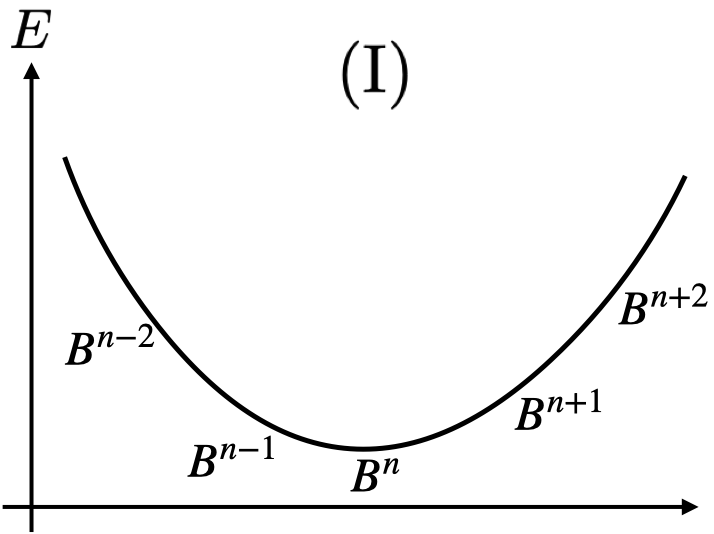
While the first and the third terms generate the eigenvalue distribution of the semi-circle law [26], the second term generated by the $-R$ charge attracts the particles to the neighborhood of $k_{2}$, and part of the $-R$ charge is screened. Therefore we can expect the following four possibilities of the eigenvalue distributions to occur:

• (I)

  For small $R$ and small $k_{2}$, there is a semi-circle-like distribution with a concentration (peak) around $k_{2}$.

• (II)

  For large $R$, all the eigenvalues concentrate around $k_{2}$.

• (III)

  For large $R$ and large $k_{2}$, there are two bunches of eigenvalues, one with a semi-circle-like distribution and the other around $k_{2}$.

• (IV)

  For small $R$ and large $k_{2}$, the eigenvalues form a semi-circle-like distribution with no concentration around $k_{2}$.

The four cases are illustrated in Figure 1. Here note that all the parameters $R,k_{1},k_{2},\alpha$ are assumed to be positive, as mentioned below (2).

Next let us discuss the large $N$ limit in a similar manner as [27]. To balance all the terms in (11), the scaling with $N$ can be determined to be

$\displaystyle\begin{split}R&=N\tilde{R},\\ k_{i}&=\sqrt{N}\tilde{k}_{i},\\ \lambda_{a}&=\sqrt{N}\tilde{\lambda}_{a},\end{split}$

(12)

where $\tilde{R}$, $\tilde{k}_{i}$, and $\tilde{\lambda}_{a}$ are supposed to be kept finite in the limit. By introducing a distribution function $\rho(\tilde{\lambda})$ for the eigenvalues, the $S_{Coul}$ in (11) can be rewritten in the large $N$ limit as

$\displaystyle S_{cont}(\rho)=N^{2}\left[-\frac{1}{2}\int_{\mathbb{R}^{2}}dxdy\,\rho(x)\rho(y)\log|x-y|+\int_{\mathbb{R}}dx\,\rho(x)\left(\tilde{R}\log|x-\tilde{k}_{2}+i\tilde{k}_{1}|+\alpha x^{2}\right)\right],$

(13)

where we have ignored an additional irrelevant constant, and have taken the normalization of $\rho$ as

$\displaystyle\int_{\mathbb{R}}dx\,\rho(x)=1$

(14)

for $\sum_{a=1}^{N}\cdots\rightarrow N\int_{\mathbb{R}}dx\,\rho(x)\cdots$.

After adding the Lagrange multiplier $\beta(\int dx\rho(x)-1)$ to take into account the constraint (14), the functional derivative of $S_{cont}$ with respect to $\rho(x)$ leads to the stationary equation,

$\displaystyle-\int_{\mathbb{R}}dy\,\rho(y)\log|x-y|+\tilde{R}\log|x-\tilde{k}_{2}+i\tilde{k}_{1}|+\alpha x^{2}+\beta=0.$

(15)

Note that this is valid only at $x$ where $\rho(x)>0$. This is because there is an implicit constraint $\rho(x)\geq 0$ and the functional derivative cannot freely be taken in the invalid region. Taking further the derivative of (15) with respect to $x$, it is obtained that

$\displaystyle\mathchoice{{\vbox{\hbox{$\textstyle-$}}\kern-4.86108pt}}{{\vbox{\hbox{$\scriptstyle-$}}\kern-3.25pt}}{{\vbox{\hbox{$\scriptscriptstyle-$}}\kern-2.29166pt}}{{\vbox{\hbox{$\scriptscriptstyle-$}}\kern-1.875pt}}\!\int_{\mathbb{R}}dy\frac{1}{x-y}\rho(y)=\frac{\tilde{R}(x-\tilde{k}_{2})}{(x-\tilde{k}_{2})^{2}+\tilde{k}_{1}^{2}}+2\alpha x,$

(16)

where the integration with a dash represents the Cauchy principal value. This equation will be treated by using the Schwinger-Dyson equation of the matrix model in the large $N$ limit in Section 4.

In this section we will study the matrix model (1) in the large $N$ limit by the Schwinger-Dyson equation. See for example [10] for some details of the techniques used in this section.

Let us define

$\displaystyle W(z):=\frac{1}{N}\left\langle{\rm Tr}\left[\frac{1}{z-M}\right]\right\rangle,$

(17)

where $z$ is a complex variable, and $\langle\cdot\rangle$ denotes the expectation value in the matrix model. Since we consider real symmetric $M$, the singularities of $W(z)$ can only be on the real axis. As we will see below, $W(z)$ has branch cuts of square roots on the real axis, and the eigenvalue density $\rho(x)$ on real $x$ is related to $W(z)$ by

$\displaystyle\rho(x)=\frac{i}{2\pi}\left[W(x+i\,\epsilon)-W(x-i\,\epsilon)\right]$

(18)

with $\epsilon=+0$.

Let us consider the Schwinger-Dyson equation,

$\displaystyle\int_{\mathbb{R}^{\#M}}\prod_{a,b=1\atop a\leq b}^{N}dM_{ab}\,D^{M}_{cd}\left\{\left(\frac{1}{z-M}\right)_{cd}e^{-S(M)}\right\}=0,$

(19)

where $D^{M}_{ab}$ denotes the partial derivative with respect to $M_{ab}$ defined by

$\displaystyle D^{M}_{ab}M_{cd}=\delta_{ac}\delta_{bd}+\delta_{bc}\delta_{ad}$

(20)

with the symmetric property of the indices of $M_{ab}$ being taken into account. By taking the derivatives on the lefthand side of (19), we obtain

$\displaystyle\begin{split}\int\prod_{a,b=1\atop a\leq b}^{N}dM_{ab}&\left\{\left(\frac{1}{z-M}\right)_{cc}\left(\frac{1}{z-M}\right)_{dd}+\left(\frac{1}{z-M}\right)_{cd}\left(\frac{1}{z-M}\right)_{dc}\right.\\ &\left.-2\left(\frac{1}{z-M}\right)_{cd}S^{\prime}(M)_{dc}\right\}e^{-S(M)}=0.\end{split}$

(21)

Let us perform the large $N$ limit given in (12), where the last one corresponds to $M\rightarrow\sqrt{N}M$ (accompanied with $z\rightarrow\sqrt{N}z$). Then, in the leading order of $N$, by assuming the factorization for the first term and ignoring the second term as sub-leading, we obtain an equation,

$\displaystyle W(z)^{2}-\frac{2}{N}\left\langle{\rm Tr}\left[\frac{\tilde{S}^{\prime}(M)}{z-M}\right]\right\rangle=0,$

(22)

where

$\displaystyle\tilde{S}^{\prime}(M)=\frac{{\tilde{R}}}{2(M-{\tilde{k}}_{2}-i{\tilde{k}}_{1})}+\frac{{\tilde{R}}}{2(M-{\tilde{k}}_{2}+i{\tilde{k}}_{1})}+2\alpha M.$

(23)

By applying the partial fraction decomposition to the last term of (22), it can further be rewritten as

$\displaystyle W(z)^{2}-2{\tilde{S}}^{\prime}(z)W(z)+{\tilde{R}}\left(\frac{W({\tilde{k}}_{2}+i{\tilde{k}}_{1})}{z-{\tilde{k}}_{2}-i{\tilde{k}}_{1}}+\frac{W({\tilde{k}}_{2}-i{\tilde{k}}_{1})}{z-{\tilde{k}}_{2}+i{\tilde{k}}_{1}}\right)+4\alpha=0.$

(24)

Therefore, the solution is given by

$\displaystyle W(z)={\tilde{S}}^{\prime}(z)-\sqrt{{\tilde{S}}^{\prime}(z)^{2}-\left[{\tilde{R}}\left(\frac{W({\tilde{k}}_{2}+i{\tilde{k}}_{1})}{z-{\tilde{k}}_{2}-i{\tilde{k}}_{1}}+\frac{W({\tilde{k}}_{2}-i{\tilde{k}}_{1})}{z-{\tilde{k}}_{2}+i{\tilde{k}}_{1}}\right)+4\alpha\right]}.$

(25)

Here the branch of the square root must appropriately be chosen as will be explained below.

The solution (25) has a complex free parameter $W({\tilde{k}}_{1}+i{\tilde{k}}_{2})$ ($W({\tilde{k}}_{1}-i{\tilde{k}}_{2})$ is its complex conjugate.). The parameter has to be tuned so that the solution becomes consistent with the expected properties of $W(z)$ defined in (17): $W(z)$ has the asymptotic behavior $W(z)\sim 1/z$ for $z\rightarrow\infty$; singularities (actually cuts) are only on the real axis. One can check that the asymptotic behavior and the absence of the poles of ${\tilde{S}}^{\prime}(z)$ in $W(z)$ are automatically satisfied by the solution (25) with an appropriate choice of the branch of the square root. However, it is difficult to tune $W({\tilde{k}}_{1}+i{\tilde{k}}_{2})$ so that all the branch cuts of (25) be located only on the real axis. This is because the content of the square root in (25) is expressed as a sixth order polynomial function of $z$ over a common denominator, and the dependence of its zeros on $W({\tilde{k}}_{1}+i{\tilde{k}}_{2})$ is too complicated to analyze. Therefore we rather take a different strategy to determine $W(z)$, which will be explained below. Whether a solution by the method below corresponds to the solution (25) with a value of $W({\tilde{k}}_{1}+i{\tilde{k}}_{2})$ can be checked afterwards for each solution.

From the discussions about the possible eigenvalue distributions in Section 3 and (18), we expect $W(z)$ has one or two cuts on the real axis. From the form of ${\tilde{S}}^{\prime}(z)$, we can assume the following forms of $W(z)$. For the cases (I), (II), or (IV) in Section 3, we assume a one-cut solution,

$\displaystyle W(z)={\tilde{S}}^{\prime}(z)-\left(\frac{c}{z-{\tilde{k}}_{2}-i{\tilde{k}}_{1}}+\frac{c^{*}}{z-{\tilde{k}}_{2}+i{\tilde{k}}_{1}}+2\alpha\right)\sqrt{z-c_{+}}\sqrt{z-c_{-}},$

(26)

where $c$ is generally complex, $c_{-}$ and $c_{+}$ are real with $c_{-}<c_{+}$, and the square roots are taken in the principal branch. From (18), $\rho(x)$ is non-zero in the region $c_{-}<x<c_{+}$. For the case (III), we assume a two-cut solution,

$\displaystyle W(z)={\tilde{S}}^{\prime}(z)-\frac{2\alpha(z-c)}{(z-{\tilde{k}}_{2})^{2}+{\tilde{k}}_{1}^{2}}\sqrt{z-c_{1}}\sqrt{z-c_{2}}\sqrt{z-c_{3}}\sqrt{z-c_{4}},$

(27)

where the parameters are assumed to be all real and satisfy $c_{1}<c_{2}<c<c_{3}<c_{4}$, and the square roots are taken in the principal branch. From (18), the eigenvalue density $\rho(x)$ is non-zero in the two regions, $[c_{1},c_{2}]$ and $[c_{3},c_{4}]$. The reason for imposing $c_{2}<c<c_{3}$ is that this condition is necessary for $\rho(x)$ to be positive in both the two regions.

For the expressions (26) and (27), it is straightforward to write down the conditions for the absence of singularities except on the real axis and the asymptotic behavior $W(z)\sim 1/z$ in $z\rightarrow\infty$. For the one-cut solution (26), we obtain

$\displaystyle\begin{split}&{\tilde{R}}/2-c\,\sqrt{{\tilde{k}}_{2}+i{\tilde{k}}_{1}-c_{+}}\,\sqrt{{\tilde{k}}_{2}+i{\tilde{k}}_{1}-c_{-}}=0,\\ &-\alpha(c_{+}+c_{-})+c+c^{*}=0,\\ &{\tilde{R}}+(c+c^{*})(c_{+}+c_{-})/2+\alpha(c_{+}-c_{-})^{2}/4-c({\tilde{k}}_{2}+i{\tilde{k}}_{1})-c^{*}({\tilde{k}}_{2}-i{\tilde{k}}_{1})=1.\end{split}$

(28)

The first condition comes from that $W(z)$ should not inherit the poles of ${\tilde{S}}^{\prime}(z)$, since they are at complex values $z=k_{2}\pm ik_{1}$. The second and the third conditions are for the asymptotic behavior of $W(z)$ to be $\sim 1/z$. Since the number of the conditions and that of the free parameters are the same, the solution is uniquely determined (There may exist some discrete sets of solutions, though).

For the two-cut solution (27), we first perform a replacement of the argument $z-{\tilde{k}}_{2}=y$ for the simplicity of the expressions, and parameterize $W(z)$ as

$\displaystyle W(y)={\tilde{S}}^{\prime}(y+{\tilde{k}}_{2})-\frac{2\alpha(y-d)}{y^{2}+{\tilde{k}}_{1}^{2}}\sqrt{y-d_{1}}\sqrt{y-d_{2}}\sqrt{y-d_{3}}\sqrt{y-d_{4}},$

(29)

where $d=c-{\tilde{k}}_{2}$ and so on, and $d_{1}<d_{2}<d<d_{3}<d_{4}$. We obtain

$\displaystyle\begin{split}&\frac{{\tilde{R}}}{2}-\frac{\alpha(i{\tilde{k}}_{1}-d)}{i{\tilde{k}}_{1}}\prod_{l=1}^{4}\sqrt{i{\tilde{k}}_{1}-d_{l}}=0,\\ &{\tilde{k}}_{2}+d+\frac{1}{2}\sum_{l=1}^{4}d_{l}=0,\\ &{\tilde{R}}+2\alpha\left(-\frac{d}{2}\sum_{l=1}^{4}d_{l}+{\tilde{k}}_{1}^{2}+\frac{1}{8}\sum_{l=1}^{4}d_{l}^{2}-\frac{1}{4}\sum_{l,m=1\atop l<m}^{4}d_{l}d_{m}\right)=1.\end{split}$

(30)

The first condition is for the absence of the poles of $\tilde{S}^{\prime}(z)$ in $W(z)$, and the last two are for the asymptotic behavior. The conditions (30) give four real conditions in total, since the first is a complex valued condition, and the latter are real. Therefore the solution has one free parameter, since the number of the parameters in (27) is five.

The presence of one free parameter in the two-cut solution is physically understandable by the aligned Coulomb gas picture of Section 3. There are two bunches of the eigenvalues, between which there exists an infinite potential barrier in the large $N$ limit. Therefore part of the eigenvalues can, freely to some extent, be moved between the two bunches without loosing the stability of the solution. This freedom gives one free parameter to the solution.

Yet one can fix this freedom by imposing that the two bunches have the same chemical potential [28]. In other words, this condition is that there is no energy cost when moving an eigenvalue from one bunch to the other. This balance between the two bunches is relevant if $N$ is not taken strictly to the infinite. To obtain the condition for the balance, let us take the aligned Coulomb gas picture of Section 3. Suppose a particle of a small charge is located at $x$ between the two bunches of the particles. Then the force $F(x)$ acting on the particle is proportional to

$\displaystyle F(x)=W(x)-{\tilde{S}}^{\prime}(x),$

(31)

where the first term represents the repulsive Coulomb forces coming from the particles contained in the bunches, and the second the forces from the negative charge and the harmonic potential. Then the energy cost of moving a particle from one bunch to the other is given by $\int_{c_{2}}^{c_{3}}dx\,F(x)$. This should vanish for the balance, and, by using (27), we obtain

$\displaystyle\begin{split}\int_{d_{2}}^{d_{3}}dy\,\frac{y-d}{y^{2}+{\tilde{k}}_{1}^{2}}\sqrt{y-d_{1}}\sqrt{y-d_{2}}\sqrt{d_{3}-y}\sqrt{d_{4}-y}=0.\end{split}$

(32)

With this additional condition, the two-cut solution is uniquely determined (There may exist some discrete sets of solutions, though).

Once a solution is obtained, one can compute the eigenvalue density by (26). We obtain

$\displaystyle\begin{split}&\rho(x)=\frac{1}{\pi}\left(\frac{c}{x-{\tilde{k}}_{2}-i{\tilde{k}}_{1}}+\frac{c^{*}}{x-{\tilde{k}}_{2}+i{\tilde{k}}_{1}}+2\alpha\right)\sqrt{c_{+}-x}\sqrt{x-c_{-}}\end{split}$

(33)

in the region $[c_{-},c_{+}]$ for the one-cut solution. Note that the positivity of $\rho(x)$ in the one-cut solution is not automatically satisfied, and there actually exist solutions with negative regions of $\rho(x)$ for some parameters. In such a case, the solutions are not correct, and other one-cut or two-cut solutions must be taken for these parameters. For the two-cut solution (27), once a solution is found with $c_{2}<c<c_{3}$, the positivity of $\rho(x)$ is automatically satisfied and

$\displaystyle\begin{split}&\rho(x)=\frac{1}{\pi}\frac{2\alpha|x-c|}{(x-{\tilde{k}}_{2})^{2}+{\tilde{k}}_{1}^{2}}\sqrt{|(x-c_{1})(x-c_{2})(x-c_{3})(x-c_{4})|}\end{split}$

(34)

for the ranges $[c_{1},c_{2}]$ and $[c_{3},c_{4}]$.

It seems difficult to obtain explicit solutions to the equations obtained in Section 4. In particular, (32) is an integral equation and would probably not be explicitly solvable. Yet, it is possible to numerically find the solutions. For demonstrations, Figure 2 shows some eigenvalue densities $\rho(x)$ which have been obtained by numerically solving the equations in Section 4 for the four cases in Section 3.

These are consistent with the results obtained from the Monte Carlo simulations of the aligned Coulomb gas system with $N=200$ in Section 3, as shown by the histograms of $\lambda_{a}$ after the rescaling (12). We can see that there are no clear qualitative differences between the profiles of (I) and (II), and therefore the classifications into (I) or (II) are rather arbitrary in the examples.

In Figure 3, the phase structure is shown in the plane of $({\tilde{k}}_{2},{\tilde{R}})$ for ${\tilde{k}}_{1}=0.1$ and $\alpha=1$. This is obtained by classifying the histograms of $\lambda_{a}$ obtained from the Monte Carlo simulations of the system (11) with $N=200$. We see that there indeed exist the four cases discussed in Section 3. A caution in this figure is that the boundary between the two cases (I) and (II) is rather arbitrary, since the profiles of (I) and (II) cannot clearly be distinguished.

Although the distinction between the cases (I) and (II) is not clear in the examples above, one can find a reason for separating the two cases in the limit ${\tilde{k}}_{1}\rightarrow+0$. To see this, let us consider the explicitly solvable case of ${\tilde{k}}_{2}=0$. This case corresponds to the one-cut solution, and the conditions (28) can straightforwardly be solved. The result of $\rho(x)$ is given by

$\displaystyle\rho(x)=\frac{1}{\pi}\left(\frac{{\tilde{R}}\,{\tilde{k}}_{1}}{(x^{2}+{\tilde{k}}_{1}^{2})\sqrt{{\tilde{k}}_{1}^{2}+a^{2}}}+2\alpha\right)\sqrt{a^{2}-x^{2}},$

(35)

where $a$ corresponds to $c_{+}$, and is determined by the equation,

$\displaystyle{\tilde{R}}-\frac{{\tilde{R}}{\tilde{k}}_{1}}{\sqrt{{\tilde{k}}_{1}^{2}+a^{2}}}+\alpha\,a^{2}=1.$

(36)

Since the lefthand side is a monotonically increasing function of $a$ with 0 at $a=0$ and $+\infty$ at $a=+\infty$, there always exists a unique solution of $a>0$ to the equation. One can also show that, by taking the partial derivatives of the lefthand side with respect to the variables, there exists no singular behavior of $a$ as a function of ${\tilde{k}}_{1}$ and ${\tilde{R}}$. This is consistent with the former statement above that the cases (I) and (II) cannot absolutely be distinguished. However, let us take the ${\tilde{k}}_{1}\rightarrow+0$ limit. In this case, the solution to (36) is explicitly given by

$\displaystyle a=\left\{\begin{array}[]{cl}\sqrt{(1-{\tilde{R}})/\alpha},&{\tilde{R}}<1,\\ 0,&{\tilde{R}}\geq 1.\end{array}\right.$

(39)

A singularity appears at ${\tilde{R}}=1$. Hence, after taking the limit ${\tilde{k}}_{1}\rightarrow+0$, (I) and (II) can clearly be distinguished by the order parameter $a$. In the next section, we will more thoroughly study the limit ${\tilde{k}}_{1}\rightarrow+0$.

While it does not seem possible to obtain explicit solutions to the equations in Section 4 for general values of the parameters, we can obtain explicit solutions by taking the ${\tilde{k}}_{1}\rightarrow+0$ limit. Fortunately, this limit is exactly consistent with our main purpose, namely, studying the case corresponding to the positive cosmological constant case of CTM, as explained in Section 2. We obtain explicit solutions for for the cases (I), (II), and (III). The case (IV) disappears in this limit, because the potential generated by the $-R$ charge becomes infinitely deep, and there always exist a bunch of eigenvalues around it.

Let us first consider the case (I). We assume ${\tilde{R}}<1$ and $c_{-}<{\tilde{k}}_{2}<c_{+}$ for the one-cut solution. The last assumption and ${\tilde{k}}_{1}\rightarrow+0$ leads to $\sqrt{{\tilde{k}}_{2}+i{\tilde{k}}_{1}-c_{+}}\,\sqrt{{\tilde{k}}_{2}+i{\tilde{k}}_{1}-c_{-}}=i\sqrt{c_{+}-{\tilde{k}}_{2}}\,\sqrt{{\tilde{k}}_{2}-c_{-}}$ in the first equation of (28), and therefore $c$ must be pure imaginary. Then the second equation leads to $c_{+}+c_{-}=0$ in the limit. Finally, with the third equation, we obtain

$\displaystyle\begin{split}&c=-\frac{i{\tilde{R}}}{2\sqrt{c_{+}-{\tilde{k}}_{2}}\,\sqrt{{\tilde{k}}_{2}-c_{-}}},\\ &c_{\pm}=\pm\sqrt{\frac{1-{\tilde{R}}}{\alpha}}\end{split}$

(40)

in the limit. Note that, because of the assumption, $c_{-}<{\tilde{k}}_{2}<c_{+}$, this solution is consistent only if

$\displaystyle 1-{\tilde{R}}-\alpha{\tilde{k}}_{2}^{2}>0.$

(41)

By putting the solution (40) to (33), $\rho(x)$ is obtained as

$\displaystyle\begin{split}\rho_{\rm(I)}(x)&=\lim_{\tilde{k}_{1}\rightarrow+0}\frac{1}{\pi}\frac{{\tilde{R}}\,{\tilde{k}}_{1}}{(x-{\tilde{k}}_{2})^{2}+{\tilde{k}}_{1}^{2}}+\frac{2\alpha}{\pi}\sqrt{(1-{\tilde{R}})/\alpha-x^{2}}\\ &={\tilde{R}}\,\delta(x-{\tilde{k}}_{2})+\frac{2\alpha}{\pi}\sqrt{(1-{\tilde{R}})/\alpha-x^{2}},\end{split}$

(42)

where the domain of $x$ is restricted to the positive region of the square root. One can check $\int_{\mathbb{R}}dx\rho_{\rm(I)}(x)=1$ holds.

The result (42) can intuitively be understood by the aligned Coulomb gas picture discussed in Section 3. In the ${\tilde{k}}_{1}\rightarrow+0$ limit, the potential generated by the charge $-R$ at $x={\tilde{k}}_{2}$ becomes infinitely deep, and some of the particles of unit charges are trapped at the location $x={\tilde{k}}_{2}$ in the limit. When ${\tilde{R}}<1$, namely, $N>R$, the number of the particles which are trapped is equal to $R$, since the particles are trapped until the $-R$ charge is totally screened. This concentration of the particles is represented by the first term of (42). Because of the total screening, the $-R$ charge is totally hidden from the remaining $N-R$ particles of unit charges, and therefore they form the semi-circle distribution because of the harmonic potential, that is represented by the second term of (42).

Let us next consider ${\tilde{R}}>1$. In this case, since $N<R$, the $-R$ charge at $x={\tilde{k}}_{2}$ can only be partially screened. This means that all the particles of unit charges are concentrated around $x={\tilde{k}}_{2}$ in the limit ${\tilde{k}}_{1}\rightarrow+0$, which corresponds to the case (II) of Section 3. Therefore, we may naturally assume the behavior,

$\displaystyle\begin{split}&c_{+}\sim{\tilde{k}}_{2}+b_{+}{\tilde{k}}_{1},\\ &c_{-}\sim{\tilde{k}}_{2}-b_{-}{\tilde{k}}_{1},\end{split}$

(43)

in the ${\tilde{k}}_{1}\rightarrow+0$ limit, where $b_{-},b_{+}>0$. Putting the assumption (43) into the first equation of (28), we obtain

$\displaystyle c\sim-\frac{i{\tilde{R}}}{2{\tilde{k}}_{1}\sqrt{b_{+}-i}\sqrt{b_{-}+i}}$

(44)

as the behavior in ${\tilde{k}}_{1}\rightarrow+0$. By putting the assumption (43) to the second equation of (28), we see that the real part of $c$ does not diverge in the limit:

$\displaystyle c+c^{*}\sim 2\alpha{\tilde{k}}_{2}.$

(45)

Therefore, this requires $b_{+}=b_{-}$ in (44). By noting that $(c+c^{*})(c_{+}+c_{-}-2{\tilde{k}}_{2})$ has lower order than ${\tilde{k}}_{1}$, the third equation of (28) leads to

$\displaystyle b_{\pm}=\frac{\sqrt{2{\tilde{R}}-1}}{{\tilde{R}}-1},$

(46)

where we have introduced a notation, $b_{\pm}:=b_{+}=b_{-}$. By putting the results into (33), we obtain

$\displaystyle\rho_{\rm(II)}(x)=\lim_{{\tilde{k}}_{1}\rightarrow+\infty}\frac{({\tilde{R}}-1)\sqrt{(b_{\pm}{\tilde{k}}_{1})^{2}-(x-{\tilde{k}}_{2})^{2}}}{\pi((x-{\tilde{k}}_{2})^{2}+{\tilde{k}}_{1}^{2})}=\delta(x-{\tilde{k}}_{2}),$

(47)

where the domain of $x$ in the middle expression is the positive region of the square root.

Let us next consider the two-cut solution in the ${\tilde{k}}_{1}\rightarrow+0$ limit. Since the potential generated by the $-R$ charge becomes infinitely deep, the case (III) with $N>R$ (${\tilde{R}}<1$) is the only possibility, and the phase (IV) does not appear. In the similar spirit as above, it is natural to assume the behavior in ${\tilde{k}}_{1}\rightarrow+0$ as

$\displaystyle\begin{split}&d_{1}\sim-b_{1},\\ &d_{2}\sim-b_{2},\\ &d_{3}\sim-b_{0}{\tilde{k}}_{1},\\ &d_{4}\sim b_{0}{\tilde{k}}_{1},\\ &d\sim-b,\end{split}$

(48)

where $b,b_{i}$ are all positive. Here, one may start with assuming different proportional coefficients for $d_{3}$ and $d_{4}$, but they turn out to be the same by the equations, as we encountered in the previous case. The ordering of $d$’s restricts $0<b<b_{2}<b_{1}$. By putting the assumptions into (30), we obtain

$\displaystyle\begin{split}&{\tilde{R}}=2\alpha b\sqrt{b_{1}b_{2}(1+b_{0}^{2})},\\ &{\tilde{k}}_{2}-b-(b_{1}+b_{2})/2=0,\\ &{\tilde{R}}+\alpha\left(-b(b_{1}+b_{2})+(b_{1}-b_{2})^{2}/4\right)=1,\end{split}$

(49)

in the limit. Solving these equations, we obtain

$\displaystyle\begin{split}&b_{0}=\sqrt{{\tilde{R}}^{2}/(4\alpha^{2}b^{2}b_{1}b_{2})-1},\\ &b_{1}={\tilde{k}}_{2}-b+\sqrt{(1-{\tilde{R}})/\alpha+2b({\tilde{k}}_{2}-b)},\\ &b_{2}={\tilde{k}}_{2}-b-\sqrt{(1-{\tilde{R}})/\alpha+2b({\tilde{k}}_{2}-b)}.\end{split}$

(50)

As discussed below (30), the solution (50) has one free parameter, which may be chosen to be $b$. It is not totally free and is restricted to a range. One condition comes from the ordering $0<b<b_{2}$ mentioned above, that leads to

$\displaystyle 0<b<\frac{1}{2}{\tilde{k}}_{2}-\sqrt{\frac{1}{6}\left(\frac{1}{2}{\tilde{k}}_{2}^{2}+\frac{1-{\tilde{R}}}{\alpha}\right)}.$

(51)

Note that the presence of this region requires

$\displaystyle\alpha{\tilde{k}}_{2}^{2}-1+{\tilde{R}}>0.$

(52)

Another condition comes from $b_{0}$ to be real in (50), that requires ${\tilde{R}}^{2}>4\alpha^{2}b^{2}b_{1}b_{2}$. To see what this inequality requires, let us introduce a function of $b$, $g(b):=4\alpha^{2}b^{2}b_{1}b_{2}$, where $b_{1},b_{2}$ are given by the functions of $b$ in (50). Then we find its derivative to be

$\displaystyle\begin{split}g^{\prime}(b)=4\alpha^{2}b\left(12(b-{\tilde{k}}_{2}/2)^{2}-{\tilde{k}}_{2}^{2}-2(1-{\tilde{R}})/\alpha\right)>0,\end{split}$

(53)

where the positivity comes from (51). Since $g(0)=0$, the condition ${\tilde{R}}^{2}>4\alpha^{2}b^{2}b_{1}b_{2}$ may also give an additional bound of the form $0<b<b_{max}$ with $g(b_{max})={\tilde{R}}^{2}$. Though the bound is not explicitly determined, an important matter here is that there exists a finite range of $b$ for a solution, if the condition (52) is satisfied.

By putting (48) and (50) to (34), and taking the ${\tilde{k}}_{1}\rightarrow+0$ limit, one obtains

$\displaystyle\begin{split}\rho_{\rm(III)}(x)=\frac{2\alpha(x+b-{\tilde{k}}_{2})\sqrt{(x+b_{1}-{\tilde{k}}_{2})(-x-b_{2}+{\tilde{k}}_{2})}}{\pi(x-{\tilde{k}}_{2})}+{\tilde{R}}\left(1-\frac{1}{\sqrt{1+b_{0}^{2}}}\right)\delta(x-{\tilde{k}}_{2}),\end{split}$

(54)

where the domain of $x$ for the first term is restricted to the positive region of the square root. One can check the normalization, $\int dx\rho_{\rm(III)}(x)=1$.

References

- [1] M. Reuter and F. Saueressig, “Quantum Gravity and the Functional Renormalization Group : The Road towards Asymptotic Safety,” Cambridge University Press, 2019.
- [2] R. Loll, “Quantum Gravity from Causal Dynamical Triangulations: A Review,” arXiv:1905.08669 [hep-th].
- [3] C. Rovelli and F. Vidotto, “Covariant Loop Quantum Gravity : An Elementary Introduction to Quantum Gravity and Spinfoam Theory,” Cambridge University Press, 2014.
- [4] S. Surya, “The causal set approach to quantum gravity,” arXiv:1903.11544 [gr-qc].
- [5] T. Konopka, F. Markopoulou and L. Smolin, “Quantum Graphity,” hep-th/0611197.
- [6] J. Ambjorn, B. Durhuus, and T. Jonsson, “Three-dimensional simplicial quantum gravity and generalized matrix models,” Mod. Phys. Lett. A06 (1991) 1133–1146.
- [7] N. Sasakura, “Tensor model for gravity and orientability of manifold,” Mod. Phys. Lett. A06 (1991) 2613–2624.
- [8] N. Godfrey and M. Gross, “Simplicial quantum gravity in more than two-dimensions,” Phys. Rev. D43 (1991) R1749–1753.
- [9] R. Gurau, “Colored Group Field Theory,” Commun. Math. Phys. 304, 69 (2011) doi:10.1007/s00220-011-1226-9 [arXiv:0907.2582 [hep-th]].
- [10] P. Di Francesco, P. H. Ginsparg and J. Zinn-Justin, “2-D Gravity and random matrices,” Phys. Rept. 254, 1-133 (1995) doi:10.1016/0370-1573(94)00084-G [arXiv:hep-th/9306153 [hep-th]].
- [11] V. Bonzom, R. Gurau, A. Riello and V. Rivasseau, “Critical behavior of colored tensor models in the large N limit,” Nucl. Phys. B 853, 174-195 (2011) doi:10.1016/j.nuclphysb.2011.07.022 [arXiv:1105.3122 [hep-th]].
- [12] R. Gurau and J. P. Ryan, “Colored Tensor Models - a review,” SIGMA 8, 020 (2012) doi:10.3842/SIGMA.2012.020 [arXiv:1109.4812 [hep-th]].
- [13] J. Ambjorn, J. Jurkiewicz and R. Loll, “Emergence of a 4-D world from causal quantum gravity,” Phys. Rev. Lett. 93, 131301 (2004) doi:10.1103/PhysRevLett.93.131301 [arXiv:hep-th/0404156 [hep-th]].
- [14] N. Sasakura, “Canonical tensor models with local time,” Int. J. Mod. Phys. A 27, 1250020 (2012) doi:10.1142/S0217751X12500200 [arXiv:1111.2790 [hep-th]].
- [15] N. Sasakura, “Uniqueness of canonical tensor model with local time,” Int. J. Mod. Phys. A 27, 1250096 (2012) doi:10.1142/S0217751X12500960 [arXiv:1203.0421 [hep-th]].
- [16] N. Sasakura, “Quantum canonical tensor model and an exact wave function,” Int. J. Mod. Phys. A 28, 1350111 (2013) doi:10.1142/S0217751X1350111X [arXiv:1305.6389 [hep-th]].
- [17] G. Narain, N. Sasakura and Y. Sato, “Physical states in the canonical tensor model from the perspective of random tensor networks,” JHEP 01, 010 (2015) doi:10.1007/JHEP01(2015)010 [arXiv:1410.2683 [hep-th]].
- [18] D. Obster and N. Sasakura, “Symmetric configurations highlighted by collective quantum coherence,” Eur. Phys. J. C 77, no.11, 783 (2017) doi:10.1140/epjc/s10052-017-5355-y [arXiv:1704.02113 [hep-th]].
- [19] D. Obster and N. Sasakura, “Emergent symmetries in the canonical tensor model,” PTEP 2018, no.4, 043A01 (2018) doi:10.1093/ptep/pty038 [arXiv:1710.07449 [hep-th]].
- [20] L. Lionni and N. Sasakura, “A random matrix model with non-pairwise contracted indices,” PTEP 2019, no. 7, 073A01 (2019) doi:10.1093/ptep/ptz057 [arXiv:1903.05944 [hep-th]].
- [21] N. Sasakura and S. Takeuchi, “Numerical and analytical analyses of a matrix model with non-pairwise contracted indices,” Eur. Phys. J. C 80, no.2, 118 (2020) doi:10.1140/epjc/s10052-019-7591-9 [arXiv:1907.06137 [hep-th]].
- [22] D. Obster and N. Sasakura, “Phases of a matrix model with non-pairwise index contractions,” doi:10.1093/ptep/ptaa085 [arXiv:2004.03152 [hep-th]].
- [23] N. Sasakura, “Numerical and analytical studies of a matrix model with non-pairwise contracted indices,” [arXiv:2004.07419 [hep-th]].
- [24] L. Paniak and N. Weiss, “Kazakov-Migdal model with logarithmic potential and the double Penner matrix model,” J. Math. Phys. 36, 2512-2530 (1995) doi:10.1063/1.531048 [arXiv:hep-th/9501037 [hep-th]].
- [25] V. A. Kazakov and P. Zinn-Justin, “Two matrix model with ABAB interaction,” Nucl. Phys. B 546, 647-668 (1999) doi:10.1016/S0550-3213(99)00015-2 [arXiv:hep-th/9808043 [hep-th]].
- [26] E. Wigner, “Characteristic vectors of bordered matrices with infinite dimensions”, Annals of Mathematics 62 (3): 548-564.
- [27] E. Brezin, C. Itzykson, G. Parisi and J. B. Zuber, “Planar Diagrams,” Commun. Math. Phys. 59, 35 (1978) doi:10.1007/BF01614153
- [28] J. Jurkiewicz, “Regularization of the One Matrix Models,” Phys. Lett. B 245, 178-184 (1990) doi:10.1016/0370-2693(90)90130-X
- [29] L. Qi, “The spectral theory of tensors (rough version),” arXiv:1201.3424 [math.SP].
- [30] N. Sasakura and Y. Sato, “Interpreting canonical tensor model in minisuperspace,” Phys. Lett. B 732, 32-35 (2014) doi:10.1016/j.physletb.2014.03.006 [arXiv:1401.2062 [hep-th]].
- [31] E. Witten, “Analytic Continuation Of Chern-Simons Theory,” AMS/IP Stud. Adv. Math. 50, 347-446 (2011) [arXiv:1001.2933 [hep-th]].