XProtoNet: Diagnosis in Chest Radiography with Global and Local Explanations
Abstract
Automated diagnosis using deep neural networks in chest radiography can help radiologists detect life-threatening diseases. However, existing methods only provide predictions without accurate explanations, undermining the trustworthiness of the diagnostic methods. Here, we present XProtoNet, a globally and locally interpretable diagnosis framework for chest radiography. XProtoNet learns representative patterns of each disease from X-ray images, which are prototypes, and makes a diagnosis on a given X-ray image based on the patterns. It predicts the area where a sign of the disease is likely to appear and compares the features in the predicted area with the prototypes. It can provide a global explanation, the prototype, and a local explanation, how the prototype contributes to the prediction of a single image. Despite the constraint for interpretability, XProtoNet achieves state-of-the-art classification performance on the public NIH chest X-ray dataset.
1 Introduction
Chest radiography is the most widely used imaging examination for diagnosing heart and other chest diseases [13]. Detecting a disease through chest radiography is a challenging task that requires professional knowledge and careful observation. Various automated diagnostic methods have been proposed to reduce the burden placed on radiologists and the likelihood of mistakes; methods using deep neural networks (DNNs) have achieved especially high levels of performance in recent decades [23, 32, 17, 10, 12]. However, the black-box characteristics of DNNs discourage users from trusting DNN predictions [22, 4]. Since medical decisions may have life-or-death consequences, medical-diagnosis applications require not only high performance but also a strong rationale for judgment. Although many automated diagnostic methods have presented localization as an explanation for prediction [32, 23, 12, 31, 20], this provides only the region on which the network is focusing within a given image, not the manner by which the network makes a decision [26].

Interpretable models, unlike conventional neural networks, are designed to operate in a human-understandable manner [26]. Case-based models learn discriminative features of each class, which are referred to as prototypes, and classify an input image by comparing its features with the prototypes [16, 3, 8]. Such models provide two types of interpretation: global and local explanations. A global explanation is a class-representative feature that is shared by multiple data points belonging to the same class [14, 25]. A local explanation, by contrast, shows how the prediction of a single input image is made. In other words, the global explanation finds the common characteristic by which the model defines each class, while the local explanation finds the reason that the model sorts a given input image into a certain class. The global explanation can be likened to the manner in which radiologists explain common signs of diseases in X-ray images, whereas the local explanation can be likened to the manner in which they diagnose individual cases by examining the part of a given X-ray image that provides information about a certain disease. This suggests that case-based models are suitable for building an interpretable automated diagnosis system.
ProtoPNet [3], which motivates our work, defines a prototype as a feature within a patch of a predefined size obtained from training images, and compares a local area in a given input image with the prototypes for classification. Despite such constraint for interpretability, it achieves performance comparable to that of conventional uninterpretable neural networks in fine-grained classification tasks. However, with a patch of a predefined size, it is difficult to reflect features that appear in a dynamic area, such as a sign of disease in medical images. For example, to identify cardiomegaly (enlargement of the heart), it is necessary to look at the whole heart [24]; to identify nodule, it is necessary to find an abnormal spot whose diameter is smaller than a threshold [7]. Depending on the fixed size of the patch, the prototypes may not sufficiently present the class-representative feature or may even present a class-irrelevant feature, leading to diagnostic failure. To address this problem, we introduce a method of training the prototypes to present class-representative features within a dynamic area (see the prototypes of each disease in Figure 1).
In this paper, we propose an interpretable automated diagnosis framework, XProtoNet, that predicts an occurrence area where a sign of a given disease is likely to appear and learns the disease-representative features of the occurrence area as prototypes. The occurrence area is adaptively predicted for each disease, enabling the prototypes to present discriminative features for diagnosis within the adaptive area for the disease. Given a chest X-ray image, XProtoNet diagnoses disease by comparing the features of the image with the learned prototypes. As shown in Figure 1, it can provide both global explanations—the discriminative features allowing the network to screen for a certain disease—and local ones—\eg, a rationale for classifying a single chest X-ray image. We evaluate our method on the public NIH chest X-ray dataset [32], which provides 14 chest-disease labels and a limited number of bounding box annotations. We also conduct further analysis of XProtoNet with a prior condition to have specific features as prototypes using the bounding box annotations. Despite strong constraints to make the network interpretable, XProtoNet achieves state-of-the-art diagnostic performance.
The main contributions of this paper can be summarized as follows:
-
We present, to the best of our knowledge, the first interpretable model for diagnosis in chest radiography that can provide both global and local explanations.
-
We propose a novel method of learning disease-representative features within a dynamic area, improving both interpretability and diagnostic performance.
-
We demonstrate that our proposed framework outperforms other state-of-the-art methods on the public NIH chest X-ray dataset.
2 Related Work
2.1 Automatic Chest X-ray Analysis
A number of researchers have attempted to identify diseases via chest radiography using DNNs. Wang et al. [32] and Rajpurkar et al. [23] proposed the use of a conventional convolutional neural network to localize disease through a class activation map [34]. Taghanaki et al. [31] utilized a variational online mask on a negligible region within the image and predicted disease using the unmasked region. Guan et al. [6] proposed a class-specific attention method and Ma et al. [20] used cross-attention with two conventional convolutional neural networks. Hermoza et al. [10] used a feature pyramid network [18] and an additional detection module to detect disease. Li et al. [17] proposed a framework to simultaneously perform disease identification and localization, exploiting a limited amount of additional supervision. Liu et al. [19], also utilizing additional supervision, proposed a method to align chest X-ray images and learn discriminative features by contrasting positive and negative samples. Some of these approaches localize the disease along with classification but cannot explain the predictive process of how this localized part contributes to model prediction. Herein, we aim to build a diagnostic framework to explain the predictive process rather than simply localize the disease.
2.2 Interpretable Models
There have been various post-hoc attempts to explain already-trained models [28, 27, 30, 2, 15], but some of them provide inaccurate explanations [29, 1]. Additionally, they only show the region where the network is looking within a given image [26]. To address this problem, several models have been proposed with structurally built-in interpretability [21, 16, 3, 8]. Since their prediction process itself is interpretable, they require no additional effort to obtain interpretation after training. A self-explaining neural network [21] obtains both concepts that are crucial in classification and the relevance of each concept separately through regularization, then combines them to make a prediction. Case-based interpretable models, mostly inspiring us, learn prototypes that present the properties of the corresponding class and identify the similarity of the features of a given input image to the learned prototypes [16, 3, 8]. Li et al. [16] used an encoder-decoder framework to extract features and visualize prototypes. Chen et al. [3] defined prototypes as a local feature of the image and visualized the prototypes by replacing them with the most similar patches of training data. Hase et al. [8] proposed training prototypes in a hierarchical structure. These works targeted classification tasks in general images, and there was no attempt to make an interpretable automated diagnosis framework for chest radiography. To this end, we propose an interpretable diagnosis model for chest radiography that learns disease-representative features within a dynamic area.
3 XProtoNet
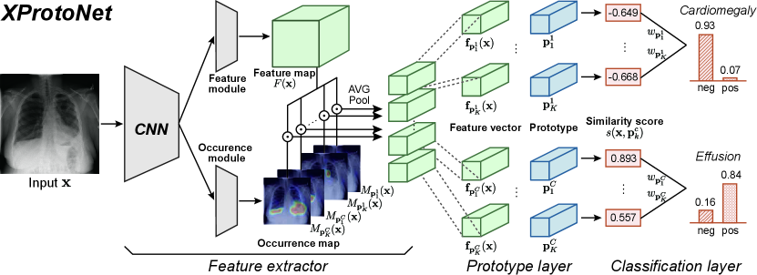
Figure 2 shows the overall architecture of our proposed framework, XProtoNet: the feature extractor, prototype layer, and classification layer. We describe the diagnostic process of XProtoNet in Section 3.1, and explain in Section 3.2 how to extract features within a dynamic area. In Section 3.3, we describe the overall training scheme.
3.1 Diagnosis Process
XProtoNet compares a given input image to learned disease-representative features to diagnose a disease. It has a set of learned prototypes for each disease , where the prototype presents a discriminative feature of disease . Given an input image , the feature extractor extracts the feature vector for each prototype , and the prototype layer calculates a similarity score between and , which are -dimensional vectors. Similarity score is calculated using cosine similarity as
| (1) |
Diagnosis from chest radiography is a multi-label classification, which is a binary classification of each class. We thus derive the prediction score of target disease by considering only the prototypes of , not the prototypes of the non-target diseases, in the classification layer. The prediction score is calculated from
| (2) |
where denotes the weight of and represents a sigmoid activation function. Similarity score indicates how similar the feature of the input image is to each prototype, and weight indicates how important each prototype is for the diagnosis. By this process, XProtoNet can diagnose the disease based on the similarity between the corresponding prototypes and the features of the input X-ray image. After the training, prototype is replaced with the most similar feature vector from the training images. This enables the prototypes to be visualized as human-interpretable training images, without an additional network for decoding the learned prototype vectors.
3.2 Extraction of Feature with Occurrence Map
When extracting feature vectors , XProtoNet considers two separate aspects of the input image: the patterns within the image and the area on which to focus to identify a certain disease. Therefore, the feature extractor of XProtoNet contains a feature module and an occurrence module for each one of the above-mentioned aspects. The feature module extracts the feature map , the latent representations of the input image , where , , and are the height, width, and dimension, respectively. The occurrence module predicts the occurrence map for each prototype , which presents where the corresponding prototype is likely to appear, that is, the focus area. Both modules consist of convolutional layers. Using occurrence map , feature vector to be compared with prototype is obtained as follows:
| (3) |
where denotes the spatial location of and (Figure 3(b)). The values of occurrence map, which are in the range , are used as the weights when pooling the feature map so that the feature vector represents a feature in the highly activated area in the occurrence map.
By pooling the feature map with the occurrence map, a class-representative feature is presented as a vector of a single size, regardless of the size or shape of the area in which the feature appears. During training, the occurrence area is optimized to cover the area where disease-representative features for each disease appear, and the prototypes become disease-representative features in an adaptive area size. As mentioned in Section 3.1, prototype is replaced with the most similar feature vector after training the feature extractor, thus the prototype can be visualized as the occurrence area of the images that the prototype vectors are replaced with.
Comparison with ProtoPNet. XProtoNet differs from ProtoPNet [3] by being able to learn features within a dynamic area. In ProtoPNet, the prototypes are compared with fixed-size feature patches from an input image (Figure 3(a)). The spatial size of the prototype is , which is smaller than the feature map. At all spatial locations in feature map , a patch from of the same size as prototype is compared to the prototype; the maximum value of the resulting similarity map becomes the final similarity score. Since a fixed-size patch in the feature map is compared with the prototypes, the prototypes can only learn representative patterns within that patch. Thus, the size of the patch greatly affects the classification performance. The prototypes may learn an insufficient portion of the class-representative pattern if the patch is not large enough, and class-irrelevant features may be presented in the prototypes if the patch is too large. The disease-representative pattern can appear in a wide range of areas, so comparing it with a fixed-size patch may limit the performance. By contrast, the feature vector in XProtoNet represents the feature throughout the wide range of area predicted by the network, and is not limited to a fixed-size region (Figure 3(b)).

3.3 Training Scheme
There are four losses in training XProtoNet: classification loss , cluster loss , separation loss , and occurrence loss .
Classification. To address the imbalance in the dataset, a weighted balance loss is used for as in [20]:
| (4) | ||||
where , the prediction score of the -th sample , and is a parameter for balance. and denote the number of negative (0) and positive (1) labels on disease , respectively. Further, denotes the target label of on disease .
Regularization for Interpretability. To allow to present the characteristics of disease , the similarity between and should be large for a positive sample and small for a negative sample. Similar to [3], we define cluster loss to maximize the similarity for positive samples and separation loss to minimize the similarity for negative samples:
| (5) | ||||
As in Eq. 4, and are weighted with the number of negative and positive samples when they are summed over all diseases and samples.
Regularization for Occurrence Map. To obtain prediction results with good interpretability, it is important to predict an appropriate occurrence map. Thus, we add two regularization terms to the training of the occurrence module. As in general object localization [33], since an affine transformation of an image does not change the relative location of a sign of the disease, it should not affect the occurrence map, either. We thus define the transformation loss for disease as
| (6) |
where denotes an affine transformation. We also add loss on the occurrence map to achieve locality of the occurrence area. It makes the occurrence area as small as possible to avoid covering more regions than necessary. The occurrence loss is thus expressed as
| (7) |
Overall Cost Function. All components of the loss are summed over all diseases, so the total loss is expressed as
| (8) |
where , , and are hyperparameters for balancing the losses.
| Methods | Atel | Card | Effu | Infi | Mass | Nodu | Pne1 | Pne2 | Cons | Edem | Emph | Fibr | P.T. | Hern | Mean |
| Baseline | 0.766 | 0.857 | 0.823 | 0.705 | 0.813 | 0.779 | 0.706 | 0.851 | 0.738 | 0.825 | 0.925 | 0.779 | 0.771 | 0.663 | 0.786 |
| Baseline | 0.767 | 0.853 | 0.826 | 0.706 | 0.813 | 0.786 | 0.705 | 0.861 | 0.737 | 0.827 | 0.927 | 0.782 | 0.776 | 0.714 | 0.792 |
| Baseline | 0.752 | 0.863 | 0.822 | 0.695 | 0.814 | 0.751 | 0.702 | 0.834 | 0.734 | 0.827 | 0.906 | 0.793 | 0.772 | 0.543 | 0.772 |
| Baseline GAP | 0.764 | 0.847 | 0.815 | 0.703 | 0.817 | 0.782 | 0.719 | 0.856 | 0.723 | 0.823 | 0.928 | 0.782 | 0.776 | 0.704 | 0.789 |
| XProtoNet (Ours) | 0.782 | 0.881 | 0.836 | 0.715 | 0.834 | 0.799 | 0.730 | 0.874 | 0.747 | 0.834 | 0.936 | 0.815 | 0.798 | 0.896 | 0.820 |
| w/o | 0.777 | 0.875 | 0.833 | 0.703 | 0.828 | 0.795 | 0.726 | 0.871 | 0.747 | 0.832 | 0.934 | 0.806 | 0.796 | 0.892 | 0.815 |


4 Experiments
4.1 Experimental Setup
Dataset. The public NIH chest X-ray dataset [32] consists of 112,120 frontal-view X-ray images with 14 disease labels from 30,805 unique patients. Experiments are conducted with two kinds of data splitting. In most of the experiments, we use an official split that sets aside 20% of the total images for the test set. We use 70% for training and 10% for validation from the remaining images. In comparison with recent methods using additional supervision (Table 3) and analysis with a prior condition to have specific prototypes (Section 4.5), we conduct a five-fold cross validation, similar to that in [17, 19]. In the official test set, there are 880 images with 984 labeled bounding boxes, provided for only eight types of diseases. We separate the total data into box-annotated and box-unannotated sets and conduct a cross-validation, where each fold has 70% of each set for training, 10% for validating, and 20% for testing. Note that we do not use the bounding box annotation during training, except for analysis with the prior condition. Patient overlap does not occur between the splits. We resize images to and normalize them with ImageNet [5] mean and standard deviation. We use data augmentation, by which images are rotated up to and scaled up or down by 20% of the image size, similar to that in [10].
Evaluation. We evaluate the diagnostic performance of XProtoNet using the area under the receiver operating characteristic curve (AUC) scores.
Experimental Details. We use ImageNet [5] pretrained conventional neural networks as a backbone (\eg, ResNet-50 [9] and DenseNet-121 [11]). The feature extractor consists of convolutional layers from the backbone network, feature module, and occurrence module. The feature and occurrence modules each consist of two convolutional layers with ReLU activation between them. The occurrence module has an additional sigmoid activation function to rescale the occurrence value to . The weights of the classification layer are initially set to 1 so that high similarity scores with the prototypes would result in a high score for the disease. and are set to 3 and 128, respectively. The batch size is set to 32. We set , , and to 0.5. Balance parameter for is set to 2. We use random resizing with ratios 0.75 and 0.875 as affine transformations for in Eq. 6.
We follow the training scheme of ProtoPNet [3]: 1) training the model, except for the convolutional layers from the pretrained network and the classification layer, for five epochs; 2) training the feature extractor and the prototype layer until the mean AUC score of the validation set does not improve for three consecutive epochs; 3) replacing the prototypes with the nearest feature vector from the training data; and 4) training the classification layer. The training steps, except for the first step, are repeated until convergence. To retain only supporting prototypes for each disease, prototypes with negative weights are pruned. More details are explained in the supplementary material.
Visualization. The occurrence maps are upsampled to the input image size and normalized with the maximum value for visualization. The prototypes are marked with contours, which depict regions in which the occurrence values are greater than a factor of 0.3 of the maximum value in the occurrence map.
4.2 Comparison with Baselines
Table 1 shows the comparison of the diagnostic performance of XProtoNet with various baselines that use different methods of comparison with the prototypes. ResNet-50 [9] is used as the backbone. Baseline refers to the method that follows ProtoPNet [3] with prototypes of spatial size , as in Figure 3(a); baseline GAP refers to the method where the feature vector is obtained by global average pooling (GAP) of the feature map without an occurrence map. The different performances of the baselines show that the performance varies greatly depending on the size of the patch. In addition, the performance of baseline GAP is similar and at times lower than that of baseline . By contrast, because XProtoNet predicts the adaptive area to compare, it achieves higher performance in all classes than the baselines: the mean AUC score of is higher than the highest baseline mean AUC score, which is . Especially, the improvement in hernia is significant (). This confirms that our proposed method of learning disease-representative features within a dynamic area is effective for diagnosis of medical images. Moreover, is also helpful in improving the performance.
Figure 4 shows the comparison of the predictions between XProtoNet and the baseline which shows the best diagnostic performance among the baselines . The cardiomegaly prototype of the baseline presents only a portion of the heart, resulting in a high similarity score (0.775) with the negative sample (Figure 4(a)). By contrast, the prototype of XProtoNet presents almost the whole area of the heart; this is more interpretable than the baseline, and the similarity score between the two occurrence areas is low (-0.369). Note that the similarity score takes a value in the range . Given the positive sample of nodule (Figure 4(b)), XProtoNet successfully detects the small nodule with a high similarity score (0.936) to the prototype, while the baseline fails. In addition, the occurrence area corresponding to the nodule prototype of XProtoNet is consistent with the ground-truth bounding box. This confirms that our proposed method shows more interpretable visualizations of the prototypes and more accurate predictions than the baseline.
4.3 Explanation with Prototypes
Figure 5 shows some examples of the global and local explanations of XProtoNet. The global explanation of XProtoNet in the diagnosis of mass can be interpreted as follows: the prototypes of mass present an abnormal spot as a major property of mass for XProtoNet; this agrees with the actual sign of lung mass [7]. In terms of the local explanation of the X-ray image (top left in Figure 5), XProtoNet predicts that the prototypes of mass are likely to appear in the large left areas of the image, which are consistent with the ground-truth bounding box. XProtoNet outputs high similarity scores between these parts and the corresponding prototypes (0.996 and 0.993), resulting in a high prediction score (0.957) for the mass. For the diagnosis on the bottom left of Figure 5, XProtoNet identifies a small region on the right within the image as the occurrence area, which is different from the first example but consistent with the actual sign. This shows that XProtoNet can dynamically predict the appropriate occurrence area.
To see whether the learned prototypes align with actual signs of diseases, we find the image that is the most similar to the prototype among the images annotated with bounding boxes. Note that those annotations are not used during training. Figure 6 shows that the occurrence area in the image is consistent with the locus of the actual sign of each disease (green boxes). This shows that the prototypes have been well-trained to present proper disease-representative features.
4.4 Diagnostic Performance
We compare the diagnostic performance of XProtoNet with recent automated diagnosis methods [32, 6, 20, 10]. Table 2 shows that XProtoNet achieves state-of-the-art performance on both ResNet-50 [9] and DenseNet-121 [11] backbones while ensuring interpretability. In comparison with recent methods implemented on ResNet-50, XProtoNet achieves the best performance for 10 out of 14 diseases. Note that Ma et al. [20] use two DenseNet-121 and Hermoza et al. [10] use a feature pyramid network [18] and DenseNet-121 as the backbone: these provide better representation than a single DenseNet-121. Compared with Guan et al. [6], who use a single DenseNet-121, the mean AUC score is improved from to .
| Methods | Atel | Card | Effu | Infi | Mass | Nodu | Pne1 | Pne2 | Cons | Edem | Emph | Fibr | P.T. | Hern | Mean |
| Backbone: ResNet-50 | |||||||||||||||
| Wang et al. [32] | 0.700 | 0.810 | 0.759 | 0.661 | 0.693 | 0.669 | 0.658 | 0.799 | 0.703 | 0.805 | 0.833 | 0.786 | 0.684 | 0.872 | 0.745 |
| Guan et al. [6] | 0.779 | 0.879 | 0.824 | 0.694 | 0.831 | 0.766 | 0.726 | 0.858 | 0.758 | 0.850 | 0.909 | 0.832 | 0.778 | 0.906 | 0.814 |
| XProtoNet (Ours) | 0.782 | 0.881 | 0.836 | 0.715 | 0.834 | 0.799 | 0.730 | 0.874 | 0.747 | 0.834 | 0.936 | 0.815 | 0.798 | 0.896 | 0.820 |
| Backbone: DenseNet-121 / DenseNet-121+* | |||||||||||||||
| Guan et al. [6] | 0.781 | 0.883 | 0.831 | 0.697 | 0.830 | 0.764 | 0.725 | 0.866 | 0.758 | 0.853 | 0.911 | 0.826 | 0.780 | 0.918 | 0.816 |
| Ma et al. [20]* | 0.777 | 0.894 | 0.829 | 0.696 | 0.838 | 0.771 | 0.722 | 0.862 | 0.750 | 0.846 | 0.908 | 0.827 | 0.779 | 0.934 | 0.817 |
| Hermoza et al. [10]* | 0.775 | 0.881 | 0.831 | 0.695 | 0.826 | 0.789 | 0.741 | 0.879 | 0.747 | 0.846 | 0.936 | 0.833 | 0.793 | 0.917 | 0.821 |
| XProtoNet (Ours) | 0.780 | 0.887 | 0.835 | 0.710 | 0.831 | 0.804 | 0.734 | 0.871 | 0.747 | 0.840 | 0.941 | 0.815 | 0.799 | 0.909 | 0.822 |
| Methods | BBox | Atel | Card | Effu | Infi | Mass | Nodu | Pne1 | Pne2 | Cons | Edem | Emph | Fibr | P.T. | Hern | Mean |
| Li et al.. [17] | ✓ | 0.80 | 0.87 | 0.87 | 0.70 | 0.83 | 0.75 | 0.67 | 0.87 | 0.80 | 0.88 | 0.91 | 0.78 | 0.79 | 0.77 | 0.81 |
| Liu et al.. [19] | ✓ | 0.79 | 0.87 | 0.88 | 0.69 | 0.81 | 0.73 | 0.75 | 0.89 | 0.79 | 0.91 | 0.93 | 0.80 | 0.80 | 0.92 | 0.83 |
| XProtoNet (Ours) | 0.83 | 0.91 | 0.89 | 0.72 | 0.87 | 0.82 | 0.76 | 0.90 | 0.80 | 0.90 | 0.94 | 0.82 | 0.82 | 0.92 | 0.85 | |
We also compare the diagnostic performance of XProtoNet to that of two recent automated diagnosis methods [17, 19] using bounding box supervision, which use ResNet-50 [9] as the backbone. Table 3 shows the performances based on a five-fold cross-validation. Despite having no additional supervision, XProtoNet achieves the best performance for most diseases.

4.5 XProtoNet with Prior Condition
As XProtoNet provides predictions based on prototypes that are exposed explicitly, we can instruct it to diagnose using specific signs of diseases by forcing the prototypes to present those signs. We conduct analysis with the prior condition that the prototypes of XProtoNet should present the features within the bounding box annotations.
XProtoNet is trained with both box-annotated and box-unannotated data. We set both and to 1.5 for the box-annotated data and both to 0.5 for the box-unannotated data. To utilize the bounding box annotations during training, we extract the feature vectors from the feature maps within the bounding boxes as , where bbox denotes the spatial location inside the bounding box. We also change loss on the occurrence map for the box-annotated data to to suppress the area outside the bounding box from being activated in the occurrence map. To enable the prototypes to present the features within the bounding boxes, the prototype vectors are replaced with their most similar feature vectors from the box-annotated data, instead of the feature vectors from the box-unannotated data.
Figure 7 shows the learned prototypes of XProtoNet trained with and without the prior condition. Owing to the constraint, the prototypes of XProtoNet trained with the prior condition present disease-representative features within the bounding box annotations. Although this can be a strong constraint for the model, there is no significant difference in the diagnostic performance: the mean AUC scores over 14 diseases of XProtoNet trained with and without the prior condition are 0.850 and 0.849, respectively. Therefore, using the prior condition, we enable XProtoNet diagnoses based on the specific features, thus rendering the system more trustworthy.

5 Conclusion
XProtoNet is an automated diagnostic framework for chest radiography that ensures human interpretability as well as high performance. XProtoNet can provide not only a local explanation for a given X-ray image but also a global explanation for each disease, which is not provided by other diagnostic methods. Despite the constraints imposed by the interpretability requirement, it achieves state-of-the-art diagnostic performance by predicting the dynamic areas where disease-representative features may be found.
With a post-hoc explanation such as localization, it is difficult to understand how a model classifies an input image. XProtoNet is one of only a very few attempts to design an explicitly interpretable model. Further research on interpretable systems using DNNs will therefore encourage the trustworthiness of the automated diagnosis system.
Acknowledgements: This work was supported by the National Research Foundation of Korea (NRF) grant funded by the Korea government (Ministry of Science and ICT) [2018R1A2B3001628], AIR Lab (AI Research Lab) in Hyundai & Kia Motor Company through HKMC-SNU AI Consortium Fund, and the BK21 FOUR program of the Education and Research Program for Future ICT Pioneers, Seoul National University in 2021.
References
- [1] Julius Adebayo, Justin Gilmer, Michael Muelly, Ian Goodfellow, Moritz Hardt, and Been Kim. Sanity checks for saliency maps. In Advances in Neural Information Processing Systems, pages 9505–9515, 2018.
- [2] Marco Ancona, Enea Ceolini, Cengiz Öztireli, and Markus Gross. Towards better understanding of gradient-based attribution methods for deep neural networks. In International Conference on Learning Representations, 2018.
- [3] Chaofan Chen, Oscar Li, Daniel Tao, Alina Barnett, Cynthia Rudin, and Jonathan K Su. This looks like that: deep learning for interpretable image recognition. In Advances in Neural Information Processing Systems, pages 8930–8941, 2019.
- [4] Travers Ching et al. Opportunities and obstacles for deep learning in biology and medicine. Journal of The Royal Society Interface, 15(141):20170387, 2018.
- [5] Jia Deng, Wei Dong, Richard Socher, Li-Jia Li, Kai Li, and Li Fei-Fei. Imagenet: A large-scale hierarchical image database. In 2009 IEEE conference on computer vision and pattern recognition, pages 248–255. Ieee, 2009.
- [6] Qingji Guan and Yaping Huang. Multi-label chest x-ray image classification via category-wise residual attention learning. Pattern Recognition Letters, 130:259–266, 2020.
- [7] David M Hansell, Alexander A Bankier, Heber MacMahon, Theresa C McLoud, Nestor L Muller, and Jacques Remy. Fleischner society: glossary of terms for thoracic imaging. Radiology, 246(3):697–722, 2008.
- [8] Peter Hase, Chaofan Chen, Oscar Li, and Cynthia Rudin. Interpretable image recognition with hierarchical prototypes. In Proceedings of the AAAI Conference on Human Computation and Crowdsourcing, volume 7, pages 32–40, 2019.
- [9] Kaiming He, Xiangyu Zhang, Shaoqing Ren, and Jian Sun. Deep residual learning for image recognition. In Proceedings of the IEEE Conference on Computer Vision and Pattern Recognition, pages 770–778, 2016.
- [10] Renato Hermoza, Gabriel Maicas, Jacinto C Nascimento, and Gustavo Carneiro. Region proposals for saliency map refinement for weakly-supervised disease localisation and classification. In International Conference on Medical Image Computing and Computer-Assisted Intervention, 2020.
- [11] Gao Huang, Zhuang Liu, Laurens Van Der Maaten, and Kilian Q Weinberger. Densely connected convolutional networks. In Proceedings of the IEEE Conference on Computer Vision and Pattern Recognition, pages 4700–4708, 2017.
- [12] Jeremy Irvin, Pranav Rajpurkar, Michael Ko, Yifan Yu, Silviana Ciurea-Ilcus, Chris Chute, Henrik Marklund, Behzad Haghgoo, Robyn Ball, Katie Shpanskaya, et al. Chexpert: A large chest radiograph dataset with uncertainty labels and expert comparison. In Proceedings of the AAAI Conference on Artificial Intelligence, volume 33, pages 590–597, 2019.
- [13] Barry Kelly. The chest radiograph. The Ulster Medical Journal, 81(3):143, 2012.
- [14] Been Kim, Martin Wattenberg, Justin Gilmer, Carrie Cai, James Wexler, Fernanda Viegas, et al. Interpretability beyond feature attribution: Quantitative testing with concept activation vectors (tcav). In International Conference on Machine Learning, pages 2668–2677. PMLR, 2018.
- [15] Pieter-Jan Kindermans, Kristof T. Schütt, Maximilian Alber, Klaus-Robert Müller, Dumitru Erhan, Been Kim, and Sven Dähne. Learning how to explain neural networks: Patternnet and patternattribution. In International Conference on Learning Representations, 2018.
- [16] Oscar Li, Hao Liu, Chaofan Chen, and Cynthia Rudin. Deep learning for case-based reasoning through prototypes: A neural network that explains its predictions. AAAI Conference on Artificial Intelligence, 2018.
- [17] Zhe Li, Chong Wang, Mei Han, Yuan Xue, Wei Wei, Li-Jia Li, and Li Fei-Fei. Thoracic disease identification and localization with limited supervision. In Proceedings of the IEEE Conference on Computer Vision and Pattern Recognition, pages 8290–8299, 2018.
- [18] Tsung-Yi Lin, Piotr Dollár, Ross Girshick, Kaiming He, Bharath Hariharan, and Serge Belongie. Feature pyramid networks for object detection. In Proceedings of the IEEE Conference on Computer Vision and Pattern Recognition, pages 2117–2125, 2017.
- [19] Jingyu Liu, Gangming Zhao, Yu Fei, Ming Zhang, Yizhou Wang, and Yizhou Yu. Align, attend and locate: Chest x-ray diagnosis via contrast induced attention network with limited supervision. In Proceedings of the IEEE International Conference on Computer Vision, pages 10632–10641, 2019.
- [20] Congbo Ma, Hu Wang, and Steven CH Hoi. Multi-label thoracic disease image classification with cross-attention networks. In International Conference on Medical Image Computing and Computer-Assisted Intervention, pages 730–738. Springer, 2019.
- [21] David Alvarez Melis and Tommi Jaakkola. Towards robust interpretability with self-explaining neural networks. In Advances in Neural Information Processing Systems, pages 7775–7784, 2018.
- [22] Tim Miller. Explanation in artificial intelligence: Insights from the social sciences. Artificial Intelligence, 267:1–38, 2019.
- [23] Pranav Rajpurkar, Jeremy Irvin, Kaylie Zhu, Brandon Yang, Hershel Mehta, Tony Duan, Daisy Ding, Aarti Bagul, Curtis Langlotz, Katie Shpanskaya, et al. Chexnet: Radiologist-level pneumonia detection on chest x-rays with deep learning. arXiv preprint arXiv:1711.05225, 2017.
- [24] Anis Rassi Jr, Anis Rassi, William C Little, Sérgio S Xavier, Sérgio G Rassi, Alexandre G Rassi, Gustavo G Rassi, Alejandro Hasslocher-Moreno, Andrea S Sousa, and Maurício I Scanavacca. Development and validation of a risk score for predicting death in chagas’ heart disease. New England Journal of Medicine, 355(8):799–808, 2006.
- [25] Marco Tulio Ribeiro, Sameer Singh, and Carlos Guestrin. ”why should i trust you?” explaining the predictions of any classifier. In Proceedings of the 22nd ACM SIGKDD international conference on knowledge discovery and data mining, pages 1135–1144, 2016.
- [26] Cynthia Rudin. Stop explaining black box machine learning models for high stakes decisions and use interpretable models instead. Nature Machine Intelligence, 1(5):206–215, 2019.
- [27] Ramprasaath R Selvaraju, Michael Cogswell, Abhishek Das, Ramakrishna Vedantam, Devi Parikh, and Dhruv Batra. Grad-cam: Visual explanations from deep networks via gradient-based localization. In Proceedings of the IEEE International Conference on Computer Vision, pages 618–626, 2017.
- [28] Karen Simonyan, Andrea Vedaldi, and Andrew Zisserman. Deep inside convolutional networks: Visualising image classification models and saliency maps. In International Conference on Learning Representations, 2014.
- [29] Leon Sixt, Maximilian Granz, and Tim Landgraf. When explanations lie: Why many modified bp attributions fail. In International Conference on Machine Learning, 2020.
- [30] Daniel Smilkov, Nikhil Thorat, Been Kim, Fernanda Viégas, and Martin Wattenberg. Smoothgrad: removing noise by adding noise. arXiv preprint arXiv:1706.03825, 2017.
- [31] Saeid Asgari Taghanaki, Mohammad Havaei, Tess Berthier, Francis Dutil, Lisa Di Jorio, Ghassan Hamarneh, and Yoshua Bengio. Infomask: Masked variational latent representation to localize chest disease. In International Conference on Medical Image Computing and Computer-Assisted Intervention, pages 739–747. Springer, 2019.
- [32] Xiaosong Wang, Yifan Peng, Le Lu, Zhiyong Lu, Mohammadhadi Bagheri, and Ronald M Summers. Chestx-ray8: Hospital-scale chest x-ray database and benchmarks on weakly-supervised classification and localization of common thorax diseases. In Proceedings of the IEEE Conference on Computer Vision and Pattern Recognition, pages 2097–2106, 2017.
- [33] Yude Wang, Jie Zhang, Meina Kan, Shiguang Shan, and Xilin Chen. Self-supervised equivariant attention mechanism for weakly supervised semantic segmentation. In Proceedings of the IEEE/CVF Conference on Computer Vision and Pattern Recognition, pages 12275–12284, 2020.
- [34] Bolei Zhou, Aditya Khosla, Agata Lapedriza, Aude Oliva, and Antonio Torralba. Learning deep features for discriminative localization. In Proceedings of the IEEE Conference on Computer Vision and Pattern Recognition, pages 2921–2929, 2016.