XKD: Cross-modal Knowledge Distillation with Domain Alignment for Video Representation Learning
Abstract
We present XKD, a novel self-supervised framework to learn meaningful representations from unlabelled videos. XKD is trained with two pseudo objectives. First, masked data reconstruction is performed to learn modality-specific representations from audio and visual streams. Next, self-supervised cross-modal knowledge distillation is performed between the two modalities through a teacher-student setup to learn complementary information. We introduce a novel domain alignment strategy to tackle domain discrepancy between audio and visual modalities enabling effective cross-modal knowledge distillation. Additionally, to develop a general-purpose network capable of handling both audio and visual streams, modality-agnostic variants of XKD are introduced, which use the same pretrained backbone for different audio and visual tasks. Our proposed cross-modal knowledge distillation improves video action classification by to on UCF101, HMDB51, and Kinetics400. Additionally, XKD improves multimodal action classification by on Kinetics-Sound. XKD shows state-of-the-art performance in sound classification on ESC50, achieving top-1 accuracy of .
1 Introduction
Self-supervised learning aims to learn meaningful representations from unlabelled data with no human supervision (Chen et al. 2020; Chen and He 2021; Misra and Maaten 2020; Grill et al. 2020; He et al. 2021). Using self-supervision, recent multimodal methods (Morgado, Vasconcelos, and Misra 2021; Alwassel et al. 2020; Morgado, Misra, and Vasconcelos 2021; Min et al. 2021; Ma et al. 2020; Sarkar and Etemad 2023) have shown great promise in learning effective representations from videos. In general, multimodal frameworks leverage the existing information in multiple data streams to learn better representations for downstream tasks toward either modality (or all). Recent audio-visual frameworks aim to perform information sharing between networks to further enrich the learned representations (Afouras, Chung, and Zisserman 2020; Chen et al. 2021; Ren et al. 2021; Aytar, Vondrick, and Torralba 2016; Albanie et al. 2018). However, effective knowledge sharing between audio and video is particularly challenging due to the inherent diversity, complexity, and domain-specific nature of each modality, as well as the existence of substantial domain gaps between them (Ren et al. 2021; Chen et al. 2021).
In this work, we aim to perform effective information sharing between audio and video streams to obtain more generalized representations for downstream tasks. To this end, we propose a novel self-supervised framework called XKD, which stands for Cross-modal Knowledge Distillation. Our approach consists of two sets of pseudo-tasks, (i) masked data modelling and (ii) cross-modal knowledge distillation. The former is performed to learn modality-specific (MS) information, while the latter distills and transfers knowledge across modalities to further enrich the learned representations. To allow for stable and effective information exchange between modalities, we introduce a domain alignment strategy. The proposed strategy involves steps (i) feature refinement that identifies ‘what to transfer’ based on cross-modal feature relevance and (ii) minimizing domain discrepancy to align the two representations. Additionally, we introduce modality-agnostic (MA) variants of our method to tackle the challenging task of learning from both modalities using a unified network (shared backbone). Modality-agnostic methods are particularly useful given their ability to accept different data streams and solve a variety of tasks using the same backbone. Moreover, they ease the challenge of designing individual models for each modality, thus attracting attention in recent studies (Girdhar et al. 2022, 2023; Akbari et al. 2021).
Inspired by the recent success of Transformers in different domains (Devlin et al. 2018; Gong, Chung, and Glass 2021a; He et al. 2021; Feichtenhofer et al. 2022), we use ViT (Dosovitskiy et al. 2020) as the backbone of our framework for both audio and visual modalities. We use the different sizes of datasets to pretrain the framework, including AudioSet, Kinetics400, and Kinetics-Sound. The pretrained backbones are then evaluated on multiple datasets on a variety of downstream tasks. More specifically, UCF101, HMDB51, and Kinetics400 are used for video-related tasks; ESC50 and FSD50K are used for audio-related tasks; and Kinetics-Sound is used for multimodal evaluation.
Our contributions are summarized as follows:
-
•
We introduce XKD, a self-supervised framework for video representation learning, which uses a novel domain alignment strategy to enable self-supervised cross-modal knowledge distillation between audio and video as two heterogeneous modalities. The proposed domain alignment strategy minimizes the domain gap and identifies the most transferable features between the two domains for effective cross-modal knowledge distillation.
-
•
Rigorous experiments and thorough ablations are performed to analyse the proposed method. XKD achieves state-of-the-art or competitive performance on a variety of downstream tasks including video action recognition, sound classification, and multimodal fusion.
-
•
Our proposed modality-agnostic variants achieve very competitive performance compared to the modality-specific ones, enabling the use of a single pretrained encoder for a variety of audio and visual downstream tasks.
The code, pretrained models, and supplementary material are available on the project website.
2 Related Work
Video self-supervised learning. Self-supervised learning has been widely used in a variety of different areas, including the challenging task of video representation learning (Schiappa, Rawat, and Shah 2022). Several prior works have attempted to learn video representations through both uni-modal (Feichtenhofer et al. 2021; Qian et al. 2021; Jing et al. 2018) as well as multimodal (Morgado, Vasconcelos, and Misra 2021; Alayrac et al. 2020; Recasens et al. 2021; Xiao, Tighe, and Modolo 2022; Han, Xie, and Zisserman 2020) pretraining. For example, prior works have explored self-supervised frameworks for learning video representations through contrastive (Morgado, Vasconcelos, and Misra 2021; Morgado, Misra, and Vasconcelos 2021; Alayrac et al. 2020), non-contrastive (Sarkar and Etemad 2023; Recasens et al. 2021), and deep clustering (Alwassel et al. 2020; Asano et al. 2020) techniques.
Masked data modelling. Inspired by the success of BERT (Devlin et al. 2018) in natural language processing, several prior works have attempted to learn meaningful representations through the reconstruction of masked (corrupted) inputs. Such methods employ encoder-decoder setups, where the encoder compresses the inputs into a lower dimension, while the decoder is trained for reconstruction. This simple approach shows promise in different domains including image (Bao, Dong, and Wei 2021; He et al. 2021; Bachmann et al. 2022), video (Wang et al. 2021; Tong et al. 2022; Feichtenhofer et al. 2022), and audio (Niizumi et al. 2022b; Gong, Chung, and Glass 2021a; Chong et al. 2022) among others.
Cross-modal knowledge distillation. The main goal of cross-modal knowledge distillation is to transfer knowledge across different modalities (Afouras, Chung, and Zisserman 2020; Dai, Das, and Bremond 2021; Chen et al. 2021; Ren et al. 2021; Aytar, Vondrick, and Torralba 2016; Albanie et al. 2018; Piergiovanni, Angelova, and Ryoo 2020). For example, (Afouras, Chung, and Zisserman 2020; Ren et al. 2021) attempted knowledge distillation between audio teachers and video students to improve visual representations. Cross-modal knowledge distillation amongst different visual modalities has been performed in (Dai, Das, and Bremond 2021), where a pretrained optical flow teacher is used to improve RGB student’s representation.
Modality-agnostic networks. While modality-specific models have been the preferred approach toward developing representation learning solutions due to their strong performance, they do not have the ability to learn from multiple modalities using the same backbone, which makes them harder to develop. Recently, (Girdhar et al. 2022; Akbari et al. 2021) introduced modality-agnostic models capable of learning different modalities using the same backbones. In our paper, we attempt to develop modality-agnostic variants of our solution which can handle very different modalities, i.e., audio and video to solve a variety of downstream tasks.

3 Method
3.1 Overview
Figure 1 presents an overview of our framework. Our method consists of two sets of autoencoders for audio () and video (). First, we train these autoencoders to reconstruct from the masked inputs, which helps the encoders ( and ) to learn modality-specific information. Next, to transfer knowledge between modalities to learn complementary information, we align the two domains by identifying the most transferable features and minimizing the domain gaps. Finally, audio () and video () teachers are employed to provide cross-modal supervision to the opposite modalities. The details of our proposed method are mentioned below.
3.2 Data Embedding
Let be given video clip , where the visual frames and audio spectrograms are denoted as and , respectively. We create ‘global’ and ‘local’ views from each modality which are then used by the teachers and students respectively. First, we apply augmentations on and to generate the global views as and . Next, we generate local views and from and respectively, where and . Specifically, is an augmented time-frequency crop of and is an augmented spatio-temporal crop of . To further elaborate, and are differently augmented than and . Both local and global views of audio and visual inputs are projected into an embedding space. For example, are reshaped into smaller patches of size , where . Similarly, we reshape the videos into smaller cuboids of size , where . Finally, the spectrogram patches and visual cuboids are flattened into vectors and linearly projected onto the embedding space, which are then fed to the encoders.
3.3 Masked Data Modelling
Inspired by the recent success and scalability of pretraining with masked reconstruction in different domains (Devlin et al. 2018; Bao, Dong, and Wei 2021; Wang et al. 2021; Gong, Chung, and Glass 2021a; Baevski et al. 2022; He et al. 2021; Niizumi et al. 2022b; Tong et al. 2022), we adopt masked data modelling in our framework to learn modality-specific representations. The masked reconstruction employs an autoencoder , which consists of an encoder and a decoder . Let be the input, which can be further expressed as a sequence of tokens , as described in Section 3.2. Here, we randomly mask some of the input tokens with , hence the masked tokens are represented as while the corrupted inputs are represented as . Further, we drop the masked tokens before feeding the input to for computational efficiency (Akbari et al. 2021; He et al. 2021). We train to reconstruct , based on input . Here, is trained to minimize the reconstruction loss as:
| (1) |
In particular, using Equation 1, we define the video and audio reconstruction losses as and for given inputs and , to train and , respectively. Here and denote video and audio autoencoders. To jointly train the audio-visual masked autoencoder, we define the final reconstruction loss as:
| (2) |
3.4 Knowledge Distillation w/ Domain Alignment
To facilitate cross-modal knowledge sharing, we adopt a teacher-student setup (Tarvainen and Valpola 2017). The teacher () and student () are comprised of a backbone and a projector head (), where the teacher and student network architectures are the same but differently parameterized. Moreover, we parameterize as , , where is the same encoder used in reconstruction (explained in the previous subsection) and is a newly added projector head. We define and as video and audio students, whereas, and are denoted as video and audio teachers.
As mentioned earlier, cross-modal knowledge distillation between audio and video is particularly difficult due to the inherent diversity, complexity, and domain-specific nature of these two modalities. To tackle this, we perform domain alignment by identifying the most transferable features and minimizing the domain discrepancy. The proposed domain alignment ensures meaningful target distributions are set by the teachers in order to perform successful cross-modal knowledge distillation.
Domain Alignment. Both the audio and video carry a rich and diverse set of information about the source. Therefore, first, we identify the most transferable features by re-weighting the teachers’ representations based on their cross-modal feature importance through a soft-selection process. Specifically, we obtain the cross-modal attention maps to calculate the cross-modal feature importance with respect to the corresponding modalities. In order to calculate the cross-modal attention maps, we first extract the modality-specific attention maps () from the last attention layers of the teacher networks as:
| (3) |
Here, denotes the query, is the key, and is the value. Specifically, is calculated as the correlation between the query () embedding of the class token (CLS) and the key () embeddings of all the other patches or cuboids. Note, denotes the number of attention heads and denotes the number of patches or cuboids. We obtain the visual attention and audio attention as per Equation 3. Next, we obtain the respective cross-modal attention maps as and as:
| (4) |
Here, and , we apply across the last dimension. Additionally, and are scaling factors, obtained as and , used to re-scale the computed cross-modal attention maps back to their original range for numerical stability. We identify the most transferable features obtained from the teachers as and , as and respectively. Here and are used to re-weight the visual and audio representations respectively. We formulate as:
| (5) |
where represents the cross-modal attention of each head and is a non-negative scalar defined as the ratio of prior and posterior energy, expressed as:
| (6) |
Next, to improve the knowledge transferability, we reduce the domain gaps by minimizing the Maximum Mean Discrepancy (MMD) (Gretton et al. 2006) loss, estimated as:
| (7) |
Here and are drawn from distributions and respectively. Additionally, is the RKHS norm (Gretton et al. 2006) and and represents the Gaussian kernel with bandwidth , written as:
| (8) |
Using Equation 7, we define domain alignment loss as:
| (9) |
Here, and refer to audio and visual representations obtained from and respectively.
Knowledge Distillation. We perform knowledge distillation between modalities to provide cross-modal supervision in order to learn complementary information. We train the student networks to match the distribution of the cross-modal teacher networks. Specifically, we train to match the distribution of , while is trained to match the distribution of . Following (Caron et al. 2021), we normalize and with a ‘mean’ calculated based on the current batch statistics, which helps the teachers’ outputs be more uniformly distributed. Additionally, to prevent abrupt updates of batch means, we slowly update the ‘means’ using an exponential moving average (EMA). Finally, we minimize the cross-entropy loss formulated as , where a and b represent the output probability distributions of and respectively. Here, the probability over distributions is obtained by using a function with the temperature parameter , where used to sharpen the distribution as:
| (10) |
Accordingly, we define the cross-modal knowledge distillation loss as:
| (11) |
3.5 Final Loss
To train XKD, we define the final loss function as the combination of reconstruction, domain alignment, and cross-modal knowledge distillation losses expressed as:
| (12) |
Here, , , and are the loss coefficients corresponding to the three loss terms, respectively. Empirically, we set , , and as , , and respectively. It should be noted that is only used to train and , not . EMA (Grill et al. 2020; Tarvainen and Valpola 2017; Chen, Xie, and He 2021) is used to slowly update and as:
| (13) |
where and are the EMA coefficients corresponding to and . We present the proposed algorithm in Alg. 1.
3.6 Modality-agnostic Variant
We take our proposed approach a step forward and attempt to train it in a modality-agnostic fashion with the goal of developing a ‘general’ network capable of handling both modalities. This is a very challenging task in the context of our work given the very diverse nature of audio and video streams. We introduce two modality-agnostic variants XKD-MATS and XKD-MAS. As the name suggests, in XKD-MATS the audio and visual teachers share their backbones, and so do the audio and visual students. In the case of XKD-MAS, the audio and visual students share their backbones, while the audio and visual teachers use modality-specific backbones. Please note that in all the setups, we use the Equation 13 to update the teachers using their respective students. Moreover, given the need to reconstruct different modalities, all of the variants use modality-specific decoders and input projection layers. The rest of the setups remain the same as the original XKD. Both variants are trained with (see Equation 12).
4 Experiments and Results
4.1 Implementation Details
Datasets. We pretrain XKD on 3 datasets of different sizes including the small-scale Kinetics-Sound (Arandjelovic and Zisserman 2017), large-scale Kinetics400 (Kay et al. 2017), and very large-scale AudioSet (Gemmeke et al. 2017). We evaluate our proposed method on a variety of downstream tasks including video action recognition, sound classification, and multimodal action classification. We use a total of datasets for downstream tasks, namely Kinetics400 (K) (Kay et al. 2017), Kinetics-Sound (KS) (Arandjelovic and Zisserman 2017), UCF101 (U) (Soomro, Zamir, and Shah 2012), HMDB51 (H) (Kuehne et al. 2011), ESC50 (E) (Piczak 2015), and FSD50K (FK) (Fonseca et al. 2022). The dataset details are provided in the supplementary material (Suppl. Mat.) Sec. A.1. Unless mentioned otherwise, Kinetics400 is used for pretraining.
Input setup. During pretraining, to save computation we downsample the video input at FPS and resize the frame resolution at . Additionally, we re-sample the audio waveforms at kHz. and generate mel-spectrograms using mel filters. Next, we create global and local views for both audio and video. We use seconds of audio-visual input for the global views. Followed by the local views are generated by taking random temporal segments of second unless stated otherwise. The final input sizes to the teachers are and . Similarly, the input sizes to the students are and , for video and audio respectively. Moreover, the inputs to the encoders for masked reconstructions are the same as the input to the teacher networks, except they are heavily masked. We use a patch size of for audio spectrograms and a cuboid size of for video input. Please see additional details in the Suppl. Mat. Sec. A.2 and A.3.
Architecture. We choose ViT (Dosovitskiy et al. 2020) as the backbone for both audio and video, due to its stability in performance across different data streams (Akbari et al. 2021). In particular, we experiment with two ViT variants ViT-B and ViT-L. By default, ViT-B is used as the video backbone for pretraining with Kinetics400 and Kinetics-Sound, whereas, ViT-Large is used when pretrained with AudioSet. In all the setups, ViT-B is used as the audio backbone. The additional details are in the Suppl. Mat. Sec. A.3 and A.4.
4.2 Effect of Cross-modal Knowledge Distillation
As discussed, the proposed XKD is pretrained to solve masked data modelling and cross-modal knowledge distillation. Therefore, to obtain an accurate understanding of the impact of cross-modal knowledge distillation, we compare XKD () with respect to the following baselines:
-
•
masked video reconstruction ()
-
•
masked audio reconstruction ()
-
•
audio-video masked autoencoder ().
We pretrain the above variants for the full training schedule of epochs and report linear evaluation results on the split-1 of downstream benchmarks.
Visual representations. The results presented in Table 4.2 show that video representations significantly benefit from the cross-modal supervision obtained through knowledge distillation. In comparison to , improves video action recognition by , , and on UCF101, HMDB51, and Kinetics-Sound, respectively. Furthermore, we challenge XKD on Kinetics400 in a linear evaluation setup which improves the top-1 accuracy by . We interestingly notice that the joint audio-visual masked reconstruction () does not make considerable improvements, e.g., it improves top-1 accuracies by only on UCf101, HMDB51, and Kinetics-Sound.
| Loss | UCF101 | HHDB51 | Kin-Sound | Kinetics400 |
|---|---|---|---|---|
| 76.1 | 51.1 | 56.8 | 30.7 | |
| 76.3 | 51.2 | 56.9 | 32.2 | |
| 84.7 | 59.3 | 70.7 | 46.4 |
| Loss | FSD50K | ESC50 |
|---|---|---|
| 44.6 | 90.0 | |
| 44.3 | 90.0 | |
| 45.8 | 91.0 |
![[Uncaptioned image]](https://cdn.awesomepapers.org/papers/41d90afe-3129-4393-9db1-7ae9afb4a0e7/x2.png)
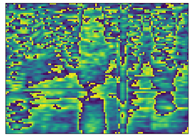
Audio representations. In Table 2, we notice that cross-modal knowledge distillation improves the performance in sound classification by and on FSD50K and ESC50 respectively. We note that the improvement is relatively less prominent compared to visual representations. Our thorough literature review in this regard reveals that a similar phenomenon has also been noticed amongst earlier works (Chen et al. 2021; Ren et al. 2021) that have attempted cross-modal knowledge distillation between audio and video in a semi-supervised setting. We conclude that while audio-to-video knowledge distillation is highly effective, video-to-audio provides a less substantial improvement. This is likely since a sharper distribution is preferred to provide supervision (Caron et al. 2021; Chen, Xie, and He 2021). As shown in Figure 2, the distribution of audio is sharper while the distribution of video is quite wider in nature. We find that such constraints can be overcome to some extent by applying aggressive sharpening of visual representations. Please find additional discussions on temperature scheduling in the Suppl. Mat. Sec. B.1. Additionally, readers are redirected to the Suppl. Mat. Sec. B.2 to B.4 for studies on EMA schedule, local views, and mask ratio.
| Loss | UCF | HMDB | Kinetics | Remarks |
|---|---|---|---|---|
| 76.3 | 51.2 | 32.2 | multimodal baseline. | |
| 76.3 | 51.2 | 32.2 | without , knowledge distillation fails. | |
| 77.8 | 51.4 | 33.7 | without , has marginal impact. | |
| 84.7 | 59.3 | 46.4 | improves the accuracy by . |
4.3 Effect of Domain Alignment
We conduct a thorough ablation study investigating the impact of domain alignment in our proposed framework, as presented in Table 3. First, without domain alignment, the model fails to perform cross-modal knowledge distillation due to domain discrepancy, and the model behaves as an audio-visual masked autoencoder. Second, quite expectedly, naively aligning the two domains without knowledge distillation has a minor impact. Last, our results exhibit that the proposed and are complementary to each other, and their combined effect significantly improves the performance, e.g., by on UCF101, HMDB51, and Kinetics400. In addition to the absence of domain alignment, we identify two more factors that could cause training instability, discussed in the Suppl. Mat. Sec. B.5 and B.6. Please see alternative design choices for domain alignment in the Suppl. Mat. Sec. B.7.
4.4 Effect of Feature Refinement ()
To study the impact of in cross-modal knowledge distillation, we modify in the final loss function (Equation 12) as . The results presented in Table 4 demonstrate that improves downstream performance by , , and on HMDB51, UCF101, and ESC50 respectively. In Figure 3, we visualize the attention from the last layer with and without , which further confirms the ability of in identifying the most transferable and key features for enhanced downstream performance. Please see alternative design choices of feature refinement Suppl. Mat. Sec. B.8.
| without | with | |
|---|---|---|
| HMDB51 | 53.5 | 59.3 |
| UCF101 | 81.0 | 84.7 |
| ESC50 | 88.0 | 91.0 |
| without refine | with refine | |
|---|---|---|
|
Crying |
![[Uncaptioned image]](https://cdn.awesomepapers.org/papers/41d90afe-3129-4393-9db1-7ae9afb4a0e7/crying_28_0without_refine.png) |
![[Uncaptioned image]](https://cdn.awesomepapers.org/papers/41d90afe-3129-4393-9db1-7ae9afb4a0e7/crying_28_0with_refine.png) |
|
Stretching |
![[Uncaptioned image]](https://cdn.awesomepapers.org/papers/41d90afe-3129-4393-9db1-7ae9afb4a0e7/stretching_leg_1_0without_refine.png) |
![[Uncaptioned image]](https://cdn.awesomepapers.org/papers/41d90afe-3129-4393-9db1-7ae9afb4a0e7/stretching_leg_1_0with_refine.png) |
| MATS | MAS | MS | |
|---|---|---|---|
| HMDB51 | 53.5 | 55.2 | 59.3 |
| UCF101 | 80.3 | 81.5 | 84.7 |
| ESC50 | 90.3 | 89.5 | 91.0 |
| Student | Teacher | |
|---|---|---|
| HMDB51 | 57.8 | 59.3 |
| UCF101 | 84.4 | 84.7 |
| ESC50 | 90.3 | 91.0 |
4.5 Comparing Modality-Agnostic vs. -Specific
In Table 6, we compare the performance of modality-agnostic (MA) variants with the modality-specific (MS) one. Amongst the MA variants, XKD-MATS works slightly better on ESC50, whereas, XKD-MAS shows better performance on both UCF101 and HMDB51. The results are promising, as these variants show minor performance drops (e.g., ) in comparison to the default XKD. Please note that such performance drops are expected as we keep the encoder size fixed for both MA and MS variants (Akbari et al. 2021). To further elaborate, while we dedicate separate backbones of M parameters to learn audio and visual representations for the MS variant, we use just one backbone of M parameters for both audio and visual modalities in the MA variants. Therefore, the network parameters or model weights become saturated relatively quickly, limiting their performance. A simple solution could be to use a larger backbone for MA variants, which could be explored in future.
4.6 Comparing Teacher vs. Student
In Table 6, we present the comparison between teachers and students. Our results exhibit that due to the slow weight update schedule using EMA (see Equation 13), the teachers become slightly stronger learners compared to the students. We study the impact of different EMA schedules (presented in the Suppl. Mat. Sec. B.2) and find that EMA coefficients as work best in our setup. As presented in Table 6, the video teacher outperforms the video student by and on UCF101 and HMDB51. Next, the audio teacher outperforms the audio student by on ESC50. Please note that by default, we use the teachers to perform downstream tasks. We present a detailed comparison between the modality-specific and modality-agnostic variants using both teacher and student encoders in the Suppl. Mat. Sec. B.9.
4.7 Scalability
We study the scalability of XKD on pretraining datasets of different sizes, similar to (Sarkar and Etemad 2023; Ma et al. 2020), i.e., Kinetics-Sound (K), Kinetics400 (K), and AudioSet (M). Additionally, we experiment with different sizes of ViT variants, i.e., ViT-B (M) and ViT-L (M). We try both ViT-B and ViT-L as the video backbone when pretrained on AudioSet. We report the linear evaluation top-1 accuracy averaged over all the splits on UCF101, HMDB51, and ESC50. Figure 4 shows that XKD continues to perform better as we increase the number of training samples and/or the size of the network. Such scalability is a much-desired property, which shows XKD can likely be scaled on even larger datasets like HowTo100M (Miech et al. 2019) or larger networks like ViT-22B (Dehghani et al. 2023). We also study the effect of longer pretraining of XKD, presented in the Suppl. Mat. Sec. B.10.

| Method | Pretrain | Mod. | UCF101 | HMDB51 | Kinetics400 | ||||||
| Lin. | FT. | Lin. | FT. | Lin. | FT. | ||||||
| AVSlowFast (2020) | K400 | VA | 77.4 | 87.0 | 44.1 | 54.6 | - | - | |||
| SeLaVi (2020) | K400 | VA | - | 83.1 | - | 47.1 | - | - | |||
| XDC (2020) | K400 | VA | - | 86.8 | - | 52.6 | - | - | |||
| CMACC (2020) | K400 | VA | - | 90.2 | - | 61.8 | - | - | |||
| AVID (2021) | K400 | VA | 72.3∗ | 87.5 | 41.4∗ | 60.8 | 44.5 | - | |||
| CMAC (2021) | K400 | VA | - | 90.3 | - | 61.1 | - | - | |||
| GDT (2021a) | K400 | VA | 70.1∗ | 90.9 | 38.5∗ | 62.3 | - | - | |||
| STiCA (2021b) | K400 | VA | - | 93.1 | - | 67.0 | - | - | |||
| CrissCross (2023) | K400 | VA | 83.9 | 91.5 | 50.0 | 64.7 | 44.5 | - | |||
| XKD | K400 | VA | 83.8 | 94.1 | 57.4 | 69.0 | 51.4 | 77.6 | |||
| XKD-MAS | K400 | VA | 81.7 | 93.4 | 55.1 | 65.9 | 50.1 | 75.9 | |||
| XKD-MATS | K400 | VA | 80.1 | 93.1 | 53.1 | 65.7 | 48.8 | 75.7 | |||
| XDC (2020) | AS | VA | 85.3 | 93.0 | 56.0 | 63.7 | - | - | |||
| MMV (2020) | AS | VA | 83.9 | 91.5 | 60.0 | 70.1 | - | - | |||
| CM-ACC (2020) | AS | VA | - | 93.5 | - | 67.2 | - | - | |||
| BraVe∗∗ (2021) | AS | VA | 90.0 | 93.6 | 63.6 | 70.8 | - | - | |||
| AVID (2021) | AS | VA | - | 91.5 | - | 64.7 | 48.9 | - | |||
| CrissCross (2023) | AS | VA | 87.7 | 92.4 | 56.2 | 67.4 | 50.1 | - | |||
| XKD | AS | VA | 88.4 | 95.8 | 62.2 | 75.7 | 56.5 | 80.1 | |||
| VideoMAE (2022) | U101/H51 | V | - | 91.3 | - | 62.6 | - | - | |||
| BEVT (2021) | K400 | V | - | - | - | - | - | 76.2 | |||
| VideoMAE (2022) | K400 | V | - | - | - | - | - | 79.0 | |||
| VideoMAE∗∗ (2022) | K400 | V | 80.0∗ | 96.1 | 54.3∗ | 73.3 | - | 80.0 | |||
| CPD (2020) | K400 | VT | - | 90.5 | - | 63.6 | - | - | |||
| CoCLR (2020) | K400 | VF | 74.5 | - | 46.1 | - | - | - | |||
| BraVe∗∗ (2021) | AS | VFA | 93.2 | 96.9 | 69.9 | 79.4 | - | - | |||
| MIL-NCE (2020) | HT | VT | - | 91.3 | - | 61.0 | - | - | |||
| VATT (2021) | AS+HT | VAT | 89.6 | - | 65.2 | - | - | 81.1 | |||
| VATT-MA (2021) | AS+HT | VAT | 84.4 | - | 63.1 | - | - | 79.9 | |||
| ELo (2020) | YT | VFA | - | 93.8 | - | 67.4 | - | - | |||
| Mod.: Modality, V: Video, A: Audio, T: Text, F: Flow. ∗computed by us using official checkpoints. ∗∗industry-level computation, e.g., VideoMAE uses vs. ours GPUs, BraVe pretrains with very high temporal resolutions (128 frames) compared to others (8-32). More comparisons with VideoMAE are in the Suppl. Mat. Sec. B.11. | |||||||||||
4.8 Video Action Recognition
Following the standard practice in (Alwassel et al. 2020; Sarkar and Etemad 2023; Ma et al. 2020), we compare XKD with other leading audio-visual self-supervised frameworks in Table 7 in both linear evaluation (Lin.) and finetuning (FT.) on UCF101, HMDB51, and Kinetics400. We note a large variability in the experiment setups amongst the prior works, however, they are included for a more inclusive and thorough comparison. We report top-1 accuracy averaged over all the splits for both UCF101 and HMDB51.
The results presented in Table 7 show that XKD outperforms or achieves competitive performance amongst the leading audio-visual self-supervised methods. For example, XKD pretrained on Kinetics400 outperforms AVID and CrissCross in linear evaluation on Kinetics400, by a very large margin. Moreover, XKD outperforms powerful state-of-the-art models like STiCA, BraVe, and CrissCross among several others when finetuned on UCF101. Additionally, XKD outperforms prior works that are pretrained with massive datasets and tri-modalities like Elo pretrained with video, audio, and optical flow from YouTube8M (YT) (Abu-El-Haija et al. 2016), compared to XKD pretrained with audio and video from AudioSet 2M. Our modality-agnostic variants also achieve encouraging results, e.g., a minor performance drop is noticed between XKD-MAS and XKD, e.g., on UCF101 and on Kinetics400, when finetuned.
| Method | Pretrain | Mod. | ESC50 | FSD50K | |||
|---|---|---|---|---|---|---|---|
| Lin. | FT. | Lin. | FT. | ||||
| XDC (2020) | K400 | VA | 78.0 | - | - | - | |
| AVID (2021) | K400 | VA | 79.1 | - | - | - | |
| STiCA (2021b) | K400 | VA | 81.1 | - | - | - | |
| CrissCross (2023) | K400 | VA | 86.8 | - | - | - | |
| XKD | K400 | VA | 89.4 | 93.6 | 45.8 | 54.1 | |
| XKD-MAS | K400 | VA | 87.3 | 92.7 | 43.0 | 52.3 | |
| XKD-MATS | K400 | VA | 88.7 | 92.9 | 43.4 | 53.8 | |
| AVTS (2018) | AS | VA | - | - | - | ||
| AVID (2021) | AS | VA | - | - | - | ||
| GDT (2021a) | AS | VA | - | - | - | ||
| CrissCross (2023) | AS | VA | - | - | - | ||
| XKD | AS | VA | 93.6 | 96.5 | 51.5 | 58.5 | |
| AudioMAE (2022) | AS | A | - | 93.6 | - | - | |
| MaskSpec (2022) | AS | A | - | 89.6 | - | - | |
| MAE-AST (2022) | AS | A | - | 90.0 | - | - | |
| BYOL-A (2022a) | AS | A | - | - | |||
| Aud. T-former (2021) | AS | A | - | - | - | 53.7 | |
| SS-AST (2021a) | AS | A | - | 88.8 | - | - | |
| PSLA (2021b) | AS | A | - | - | - | 55.8 | |
| VATT (2021) | AS+HT | VAT | - | - | - | ||
| VATT-MA (2021) | AS+HT | VAT | - | - | - | ||
| PaSST(SL) (2021) | AS+IN | AI | - | 95.5 | - | 58.4 | |
| Here, I: Image, IN: ImageNet (Russakovsky et al. 2015). | |||||||
4.9 Sound Classification
In Table 8, we compare the performance of our proposed method using linear evaluation (Lin.) and finetuning (FT.) on sound classification using popular audio benchmarks ESC50 and FSD50K. Following (Fonseca et al. 2022; Piczak 2015), we report top-1 accuracy averaged over all the splits on ESC50 and mean average precision on FSD50K. XKD outperforms prior works like XDC, AVID, and CrissCross on ESC50 in both linear evaluation and finetuning. Moreover, XKD and its MA variants outperform VATT and VATT-MA on ESC50 by and , even though VATT is pretrained with M videos, compared to XKD which is only trained on K samples. Additionally, when evaluated on FSD50K, XKD outperforms BYOL-A, AudioTransformer, and PSLA among others. Lastly, XKD shows state-of-the-art performance on ESC50, achieving top-1 finetuned accuracy of when pretrained with AudioSet.
| Method | Audio + Video |
|---|---|
| CrissCross | 66.7 |
| (AV-MAE) | 75.7 |
| XKD | 81.2 |
| XKD-MAS | 78.8 |
| XKD-MATS | 78.3 |
4.10 Multimodal Fusion
Following (Sarkar and Etemad 2023), we evaluate XKD in multimodal action classification using Kinetics-Sound. We extract fixed audio and visual embeddings from the pretrained encoders and concatenate them together (i.e., late fusion), followed by a linear SVM classifier is trained and top-1 accuracy is reported. The results presented in Table 9 show that XKD outperforms CrissCross by and baseline audio-visual masked autoencoder () by .
4.11 In-painting.
We present reconstruction examples in Figure 5, which shows that XKD retains its reconstruction ability even when a very high masking ratio is applied, for both audio and video modalities. This makes XKD also suitable for in-painting tasks. More examples are in the Suppl. Mat. Sec. C.2.
| Original | Masked | Reconstructed | |
|---|---|---|---|
|
Video |
 |
 |
 |
|
Audio |
 |
 |
 |
5 Summary
In this work, we propose XKD, a novel self-supervised framework to improve video representation learning using cross-modal knowledge distillation. To effectively transfer knowledge between audio and video modalities, XKD aligns the two domains by identifying the most transferable features and minimizing the domain gaps. Our study shows that cross-modal knowledge distillation significantly improves video representations on a variety of benchmarks. Additionally, to develop a general network with the ability to process different modalities, we introduce modality-agnostic variants of XKD which show promising results in handling both audio and video using the same backbone. We believe that our approach can be further expanded to perform cross-modal knowledge distillation between other modalities as well (e.g., vision and language), which could be investigated in the future.
Acknowledgments
We are grateful to the Bank of Montreal and Mitacs for funding this research. We are thankful to SciNet HPC Consortium for helping with the computation resources.
References
- Abu-El-Haija et al. (2016) Abu-El-Haija, S.; Kothari, N.; Lee, J.; Natsev, P.; Toderici, G.; Varadarajan, B.; and Vijayanarasimhan, S. 2016. Youtube-8m: A large-scale video classification benchmark. arXiv preprint arXiv:1609.08675.
- Afouras, Chung, and Zisserman (2020) Afouras, T.; Chung, J. S.; and Zisserman, A. 2020. Asr is all you need: Cross-modal distillation for lip reading. In ICASSP, 2143–2147. IEEE.
- Akbari et al. (2021) Akbari, H.; Yuan, L.; Qian, R.; Chuang, W.-H.; Chang, S.-F.; Cui, Y.; and Gong, B. 2021. Vatt: Transformers for multimodal self-supervised learning from raw video, audio and text. NeurIPS, 34.
- Alayrac et al. (2020) Alayrac, J.-B.; Recasens, A.; Schneider, R.; Arandjelovic, R.; Ramapuram, J.; De Fauw, J.; Smaira, L.; Dieleman, S.; and Zisserman, A. 2020. Self-Supervised MultiModal Versatile Networks. NeurIPS, 2(6): 7.
- Albanie et al. (2018) Albanie, S.; Nagrani, A.; Vedaldi, A.; and Zisserman, A. 2018. Emotion recognition in speech using cross-modal transfer in the wild. In ACM Multimedia, 292–301.
- Alwassel et al. (2020) Alwassel, H.; Mahajan, D.; Korbar, B.; Torresani, L.; Ghanem, B.; and Tran, D. 2020. Self-Supervised Learning by Cross-Modal Audio-Video Clustering. NeurIPS, 33.
- Arandjelovic and Zisserman (2017) Arandjelovic, R.; and Zisserman, A. 2017. Look, listen and learn. In ICCV, 609–617.
- Asano et al. (2020) Asano, Y. M.; Patrick, M.; Rupprecht, C.; and Vedaldi, A. 2020. Labelling unlabelled videos from scratch with multi-modal self-supervision. In NeurIPS.
- Aytar, Vondrick, and Torralba (2016) Aytar, Y.; Vondrick, C.; and Torralba, A. 2016. Soundnet: Learning sound representations from unlabeled video. NeurIPS, 29.
- Baade, Peng, and Harwath (2022) Baade, A.; Peng, P.; and Harwath, D. 2022. Mae-ast: Masked autoencoding audio spectrogram transformer. arXiv preprint arXiv:2203.16691.
- Bachmann et al. (2022) Bachmann, R.; Mizrahi, D.; Atanov, A.; and Zamir, A. 2022. MultiMAE: Multi-modal Multi-task Masked Autoencoders. arXiv preprint arXiv:2204.01678.
- Baevski et al. (2022) Baevski, A.; Hsu, W.-N.; Xu, Q.; Babu, A.; Gu, J.; and Auli, M. 2022. Data2vec: A general framework for self-supervised learning in speech, vision and language. arXiv preprint arXiv:2202.03555.
- Bao, Dong, and Wei (2021) Bao, H.; Dong, L.; and Wei, F. 2021. Beit: Bert pre-training of image transformers. arXiv preprint arXiv:2106.08254.
- Caron et al. (2021) Caron, M.; Touvron, H.; Misra, I.; Jégou, H.; Mairal, J.; Bojanowski, P.; and Joulin, A. 2021. Emerging properties in self-supervised vision transformers. In ICCV, 9650–9660.
- Chen et al. (2020) Chen, T.; Kornblith, S.; Norouzi, M.; and Hinton, G. 2020. A simple framework for contrastive learning of visual representations. In ICML, 1597–1607.
- Chen and He (2021) Chen, X.; and He, K. 2021. Exploring simple siamese representation learning. In CVPR, 15750–15758.
- Chen, Xie, and He (2021) Chen, X.; Xie, S.; and He, K. 2021. An empirical study of training self-supervised vision transformers. In Proceedings of the IEEE/CVF International Conference on Computer Vision, 9640–9649.
- Chen et al. (2021) Chen, Y.; Xian, Y.; Koepke, A.; Shan, Y.; and Akata, Z. 2021. Distilling audio-visual knowledge by compositional contrastive learning. In CVPR, 7016–7025.
- Chong et al. (2022) Chong, D.; Wang, H.; Zhou, P.; and Zeng, Q. 2022. Masked Spectrogram Prediction For Self-Supervised Audio Pre-Training. arXiv preprint arXiv:2204.12768.
- Cubuk et al. (2020) Cubuk, E. D.; Zoph, B.; Shlens, J.; and Le, Q. V. 2020. Randaugment: Practical automated data augmentation with a reduced search space. In CVPRW, 702–703.
- Dai, Das, and Bremond (2021) Dai, R.; Das, S.; and Bremond, F. 2021. Learning an augmented rgb representation with cross-modal knowledge distillation for action detection. In ICCV, 13053–13064.
- Dehghani et al. (2023) Dehghani, M.; Djolonga, J.; Mustafa, B.; Padlewski, P.; Heek, J.; Gilmer, J.; Steiner, A. P.; Caron, M.; Geirhos, R.; Alabdulmohsin, I.; et al. 2023. Scaling vision transformers to 22 billion parameters. In ICML, 7480–7512. PMLR.
- Devlin et al. (2018) Devlin, J.; Chang, M.-W.; Lee, K.; and Toutanova, K. 2018. Bert: Pre-training of deep bidirectional transformers for language understanding. arXiv preprint arXiv:1810.04805.
- Dosovitskiy et al. (2020) Dosovitskiy, A.; Beyer, L.; Kolesnikov, A.; Weissenborn, D.; Zhai, X.; Unterthiner, T.; Dehghani, M.; Minderer, M.; Heigold, G.; Gelly, S.; et al. 2020. An image is worth 16x16 words: Transformers for image recognition at scale. arXiv preprint arXiv:2010.11929.
- Feichtenhofer et al. (2022) Feichtenhofer, C.; Fan, H.; Li, Y.; and He, K. 2022. Masked Autoencoders As Spatiotemporal Learners. arXiv preprint arXiv:2205.09113.
- Feichtenhofer et al. (2021) Feichtenhofer, C.; Fan, H.; Xiong, B.; Girshick, R.; and He, K. 2021. A large-scale study on unsupervised spatiotemporal representation learning. In CVPR, 3299–3309.
- Fonseca et al. (2022) Fonseca, E.; Favory, X.; Pons, J.; Font, F.; and Serra, X. 2022. FSD50K: an open dataset of human-labeled sound events. IEEE/ACM Transactions on Audio, Speech, and Language Processing, 30: 829–852.
- Gemmeke et al. (2017) Gemmeke, J. F.; Ellis, D. P.; Freedman, D.; Jansen, A.; Lawrence, W.; Moore, R. C.; Plakal, M.; and Ritter, M. 2017. Audio set: An ontology and human-labeled dataset for audio events. In ICASSP, 776–780.
- Girdhar et al. (2023) Girdhar, R.; El-Nouby, A.; Liu, Z.; Singh, M.; Alwala, K. V.; Joulin, A.; and Misra, I. 2023. Imagebind: One embedding space to bind them all. In CVPR, 15180–15190.
- Girdhar et al. (2022) Girdhar, R.; Singh, M.; Ravi, N.; van der Maaten, L.; Joulin, A.; and Misra, I. 2022. Omnivore: A single model for many visual modalities. In CVPR, 16102–16112.
- Gong, Chung, and Glass (2021a) Gong, Y.; Chung, Y.-A.; and Glass, J. 2021a. Ast: Audio spectrogram transformer. arXiv preprint arXiv:2104.01778.
- Gong, Chung, and Glass (2021b) Gong, Y.; Chung, Y.-A.; and Glass, J. 2021b. Psla: Improving audio tagging with pretraining, sampling, labeling, and aggregation. IEEE/ACM Transactions on Audio, Speech, and Language Processing, 29: 3292–3306.
- Gretton et al. (2006) Gretton, A.; Borgwardt, K.; Rasch, M.; Schölkopf, B.; and Smola, A. 2006. A kernel method for the two-sample-problem. NeurIPS, 19.
- Grill et al. (2020) Grill, J.-B.; Strub, F.; Altché, F.; Tallec, C.; Richemond, P.; Buchatskaya, E.; Doersch, C.; Pires, B.; Guo, Z.; Azar, M.; et al. 2020. Bootstrap Your Own Latent: A new approach to self-supervised learning. In NeurIPS.
- Han, Xie, and Zisserman (2020) Han, T.; Xie, W.; and Zisserman, A. 2020. Self-supervised Co-training for Video Representation Learning. In NeurIPS.
- He et al. (2021) He, K.; Chen, X.; Xie, S.; Li, Y.; Dollár, P.; and Girshick, R. 2021. Masked autoencoders are scalable vision learners. arXiv preprint arXiv:2111.06377.
- Huang et al. (2022) Huang, P.-Y.; Xu, H.; Li, J.; Baevski, A.; Auli, M.; Galuba, W.; Metze, F.; and Feichtenhofer, C. 2022. Masked autoencoders that listen. NeurIPS, 35: 28708–28720.
- Jing et al. (2018) Jing, L.; Yang, X.; Liu, J.; and Tian, Y. 2018. Self-supervised spatiotemporal feature learning via video rotation prediction. arXiv preprint arXiv:1811.11387.
- Kay et al. (2017) Kay, W.; Carreira, J.; Simonyan, K.; Zhang, B.; Hillier, C.; Vijayanarasimhan, S.; Viola, F.; Green, T.; Back, T.; Natsev, P.; et al. 2017. The kinetics human action video dataset. arXiv preprint arXiv:1705.06950.
- Korbar, Tran, and Torresani (2018) Korbar, B.; Tran, D.; and Torresani, L. 2018. Cooperative learning of audio and video models from self-supervised synchronization. In NeruIPS, 7774–7785.
- Koutini et al. (2021) Koutini, K.; Schlüter, J.; Eghbal-zadeh, H.; and Widmer, G. 2021. Efficient training of audio transformers with patchout. arXiv preprint arXiv:2110.05069.
- Kuehne et al. (2011) Kuehne, H.; Jhuang, H.; Garrote, E.; Poggio, T.; and Serre, T. 2011. HMDB: a large video database for human motion recognition. In ICCV, 2556–2563.
- Li and Wang (2020) Li, T.; and Wang, L. 2020. Learning spatiotemporal features via video and text pair discrimination. arXiv preprint arXiv:2001.05691.
- Loshchilov and Hutter (2017) Loshchilov, I.; and Hutter, F. 2017. Decoupled weight decay regularization. arXiv preprint arXiv:1711.05101.
- Ma et al. (2020) Ma, S.; Zeng, Z.; McDuff, D.; and Song, Y. 2020. Active Contrastive Learning of Audio-Visual Video Representations. In ICLR.
- Micikevicius et al. (2018) Micikevicius, P.; Narang, S.; Alben, J.; Diamos, G.; Elsen, E.; Garcia, D.; Ginsburg, B.; Houston, M.; Kuchaiev, O.; Venkatesh, G.; et al. 2018. Mixed Precision Training. In ICLR.
- Miech et al. (2020) Miech, A.; Alayrac, J.-B.; Smaira, L.; Laptev, I.; Sivic, J.; and Zisserman, A. 2020. End-to-end learning of visual representations from uncurated instructional videos. In CVPR, 9879–9889.
- Miech et al. (2019) Miech, A.; Zhukov, D.; Alayrac, J.-B.; Tapaswi, M.; Laptev, I.; and Sivic, J. 2019. HowTo100M: Learning a Text-Video Embedding by Watching Hundred Million Narrated Video Clips. In ICCV.
- Min et al. (2021) Min, S.; Dai, Q.; Xie, H.; Gan, C.; Zhang, Y.; and Wang, J. 2021. Cross-Modal Attention Consistency for Video-Audio Unsupervised Learning. arXiv preprint arXiv:2106.06939.
- Misra and Maaten (2020) Misra, I.; and Maaten, L. v. d. 2020. Self-supervised learning of pretext-invariant representations. In CVPR, 6707–6717.
- Morgado, Misra, and Vasconcelos (2021) Morgado, P.; Misra, I.; and Vasconcelos, N. 2021. Robust Audio-Visual Instance Discrimination. In CVPR, 12934–12945.
- Morgado, Vasconcelos, and Misra (2021) Morgado, P.; Vasconcelos, N.; and Misra, I. 2021. Audio-visual instance discrimination with cross-modal agreement. In CVPR, 12475–12486.
- Niizumi et al. (2022a) Niizumi, D.; Takeuchi, D.; Ohishi, Y.; Harada, N.; and Kashino, K. 2022a. BYOL for Audio: Exploring Pre-trained General-purpose Audio Representations. arXiv preprint arXiv:2204.07402.
- Niizumi et al. (2022b) Niizumi, D.; Takeuchi, D.; Ohishi, Y.; Harada, N.; and Kashino, K. 2022b. Masked Spectrogram Modeling using Masked Autoencoders for Learning General-purpose Audio Representation. arXiv preprint arXiv:2204.12260.
- Patrick et al. (2021a) Patrick, M.; Asano, Y. M.; Kuznetsova, P.; Fong, R.; Henriques, J. F.; Zweig, G.; and Vedaldi, A. 2021a. Multi-modal Self-Supervision from Generalized Data Transformations. ICCV.
- Patrick et al. (2021b) Patrick, M.; Huang, P.-Y.; Misra, I.; Metze, F.; Vedaldi, A.; Asano, Y. M.; and Henriques, J. F. 2021b. Space-Time Crop & Attend: Improving Cross-modal Video Representation Learning. In ICCV, 10560–10572.
- Piczak (2015) Piczak, K. J. 2015. ESC: Dataset for Environmental Sound Classification. In ACM Multimedia, 1015–1018. .
- Piergiovanni, Angelova, and Ryoo (2020) Piergiovanni, A.; Angelova, A.; and Ryoo, M. S. 2020. Evolving losses for unsupervised video representation learning. In CVPR, 133–142.
- Qian et al. (2021) Qian, R.; Meng, T.; Gong, B.; Yang, M.-H.; Wang, H.; Belongie, S.; and Cui, Y. 2021. Spatiotemporal contrastive video representation learning. In CVPR, 6964–6974.
- Recasens et al. (2021) Recasens, A.; Luc, P.; Alayrac, J.-B.; Wang, L.; Strub, F.; Tallec, C.; Malinowski, M.; Pătrăucean, V.; Altché, F.; Valko, M.; et al. 2021. Broaden your views for self-supervised video learning. In ICCV, 1255–1265.
- Reddi, Kale, and Kumar (2019) Reddi, S. J.; Kale, S.; and Kumar, S. 2019. On the convergence of adam and beyond. arXiv preprint arXiv:1904.09237.
- Ren et al. (2021) Ren, S.; Du, Y.; Lv, J.; Han, G.; and He, S. 2021. Learning from the master: Distilling cross-modal advanced knowledge for lip reading. In CVPR, 13325–13333.
- Russakovsky et al. (2015) Russakovsky, O.; Deng, J.; Su, H.; Krause, J.; Satheesh, S.; Ma, S.; Huang, Z.; Karpathy, A.; Khosla, A.; Bernstein, M.; et al. 2015. Imagenet large scale visual recognition challenge. IJCV, 115: 211–252.
- Sarkar and Etemad (2023) Sarkar, P.; and Etemad, A. 2023. Self-supervised audio-visual representation learning with relaxed cross-modal synchronicity. In AAAI, volume 37, 9723–9732.
- Schiappa, Rawat, and Shah (2022) Schiappa, M. C.; Rawat, Y. S.; and Shah, M. 2022. Self-supervised learning for videos: A survey. arXiv preprint arXiv:2207.00419.
- Soomro, Zamir, and Shah (2012) Soomro, K.; Zamir, A. R.; and Shah, M. 2012. UCF101: A dataset of 101 human actions classes from videos in the wild. arXiv preprint arXiv:1212.0402.
- Szegedy et al. (2016) Szegedy, C.; Vanhoucke, V.; Ioffe, S.; Shlens, J.; and Wojna, Z. 2016. Rethinking the inception architecture for computer vision. In CVPR, 2818–2826.
- Tarvainen and Valpola (2017) Tarvainen, A.; and Valpola, H. 2017. Mean teachers are better role models: Weight-averaged consistency targets improve semi-supervised deep learning results. NeurIPS, 30.
- Tong et al. (2022) Tong, Z.; Song, Y.; Wang, J.; and Wang, L. 2022. VideoMAE: Masked Autoencoders are Data-Efficient Learners for Self-Supervised Video Pre-Training. arXiv preprint arXiv:2203.12602.
- Verma and Berger (2021) Verma, P.; and Berger, J. 2021. Audio transformers: Transformer architectures for large scale audio understanding. adieu convolutions. arXiv preprint arXiv:2105.00335.
- Wang et al. (2021) Wang, R.; Chen, D.; Wu, Z.; Chen, Y.; Dai, X.; Liu, M.; Jiang, Y.-G.; Zhou, L.; and Yuan, L. 2021. Bevt: Bert pretraining of video transformers. arXiv preprint arXiv:2112.01529.
- Xiao et al. (2020) Xiao, F.; Lee, Y. J.; Grauman, K.; Malik, J.; and Feichtenhofer, C. 2020. Audiovisual slowfast networks for video recognition. arXiv preprint arXiv:2001.08740.
- Xiao, Tighe, and Modolo (2022) Xiao, F.; Tighe, J.; and Modolo, D. 2022. MaCLR: Motion-Aware Contrastive Learning of Representations for Videos. In ECCV, 353–370. Springer.
- Yun et al. (2019) Yun, S.; Han, D.; Oh, S. J.; Chun, S.; Choe, J.; and Yoo, Y. 2019. Cutmix: Regularization strategy to train strong classifiers with localizable features. In ICCV, 6023–6032.
- Zhang et al. (2017) Zhang, H.; Cisse, M.; Dauphin, Y. N.; and Lopez-Paz, D. 2017. mixup: Beyond empirical risk minimization. arXiv preprint arXiv:1710.09412.
Supplementary Material
The organization of the supplementary material is as follows:
- •
-
•
B: Additional Experiments and Results
-
–
B.1 Effect of temperature schedules
-
–
B.2 Effect of different EMA schedules
-
–
B.3 Effect of local views
-
–
B.4 Effect of different mask ratio
-
–
B.5 Avoiding collapse and training instability
-
–
B.6 Design choices for projector head
-
–
B.7 Design choices for domain alignment
-
–
B.8 Design choices for feature refinement
-
–
B.9 Comparing different variants of XKD
-
–
B.10 Training schedule
-
–
B.11 Detailed comparison with VideoMAE
-
–
- •
Appendix A Implementation Details
A.1 Datasets
The details of the datasets are presented.
Kinetics400. Kinetics400(Kay et al. 2017) is a large-scale action recognition audio-visual dataset consisting of action classes. It has a total of K video clips with an average duration of seconds. Following (Sarkar and Etemad 2023; Alwassel et al. 2020; Morgado, Vasconcelos, and Misra 2021; Tong et al. 2022; Feichtenhofer et al. 2022), we use the Kinetics400 for both pretraining and downstream evaluation.
AudioSet. AudioSet (Gemmeke et al. 2017) is a very large-scale audio-visual dataset comprised of M videos and collected from YouTube. The samples from AudioSet are of average duration of seconds and spread over audio events. We use AudioSet to conduct experiments on large-scale pretraining. Please note that none of the labels are used in pretraining.
UCF101. UCF101(Soomro, Zamir, and Shah 2012) is a popular action recognition dataset used for downstream evaluation. It consists of a total of K clips of an average duration of seconds and spread over action classes. We use UCF101 for downstream evaluation on video action recognition.
HMDB51. HMDB51 (Kuehne et al. 2011) is one of earlier video action recognition datasets. It contains K video clips distributed over action classes. HMDB51 is used for downstream evaluation on video action recognition.
Kinetics-Sound. Kinetics-Sound(Arandjelovic and Zisserman 2017) is originally a subset of Kinetics400, which has a total of K video clips consisting of action classes. Following (Sarkar and Etemad 2023), we use Kinetics-Sound for multimodal action classification by late fusion. We particularly choose Kinetics-Sound for multimodal evaluation as it consists of hand-picked samples from Kinetics400 which are prominently manifested both audibly and visually. In addition to downstream evaluation, Kinetics-Sound is also used to conduct experiments on small-scale pretraining.
ESC50. ESC50 is a popular sound classification dataset that consists of a total of K samples of environmental sound classes, with an average duration of seconds. Following (Akbari et al. 2021; Sarkar and Etemad 2023; Morgado, Vasconcelos, and Misra 2021; Recasens et al. 2021), we use ESC50 for downstream evaluation of audio representations.
FSD50K. FSD50K is a popular audio dataset of human-labeled sound events, which consists of K audio samples distributed over classes. Moreover, FSD50K is a multi-labeled dataset, where samples are between to seconds. Following (Niizumi et al. 2022a) We use FSD50K for downstream evaluation of audio representations.
A.2 Augmentation
We adopt standard augmentation strategies (Sarkar and Etemad 2023; Chen et al. 2020; Niizumi et al. 2022a) to create the global and local views from the raw audio and visual streams. Particularly, we apply Multi-scale crop, Color Jitter, and Random Horizontal Flip to create global visual views. To create local views, we apply Gray Scale and Gaussian Blur, in addition to the augmentations applied on the global views with minor changes in the augmentation parameters. For example, different from global visual views, we apply aggressive cropping to create local visual views. The details of the augmentation parameters are presented in Table S1. Next, Volume Jitter is applied to the audio stream to create the global audio views. We apply Random Crop in addition to the Volume Jitter to create the local audio views. The details of the audio augmentation parameters are presented in Table S2.
| Augmentation | Param | Global View | Local View | Linear Eval. |
|---|---|---|---|---|
| Multi-Scale Crop | Crop Scale | [0.2, 1] | [0.08, 0.4] | [0.08, 1] |
| Horizontal Flip | Probability | 0.5 | 0.5 | 0.5 |
| Color Jitter | Brightness | 0.4 | 0.4 | 0.4 |
| Contrast | 0.4 | 0.4 | 0.4 | |
| Saturation | 0.4 | 0.4 | 0.4 | |
| Hue | 0.2 | 0.2 | 0.2 | |
| Gray Scale | Probability | n/a | 0.2 | 0.2 |
| Gaussian Blur | Probability | n/a | 0.5 | n/a |
| Augmentation | Param | Global View | Local View | Linear Eval. |
|---|---|---|---|---|
| Volume Jitter | Scale | 0.1 | 0.2 | 0.1 |
| Random Crop | Range | n/a | [0.6, 1.5] | n/a |
| Crop Scale | n/a | [1, 1.5] | n/a |
A.3 Pretraining
We train XKD using an AdamW (Loshchilov and Hutter 2017; Reddi, Kale, and Kumar 2019) optimizer and warm-up cosine learning rate scheduler. During ablation studies, the models are trained for epochs using Kinetics400. We use ViT-B (Dosovitskiy et al. 2020) as the backbone for both audio and visual modalities. Following (He et al. 2021), we use a shallow decoder for reconstruction and adopt a similar projector head to the one proposed in (Caron et al. 2021). Please see the additional architecture details in Table S3. We perform distributed training with a batch size of using NVIDIA V100 GB GPUs in parallel. As mentioned in Table S3, we use visual frames with resolutions of and , such lower resolutions allow us to train the proposed XKD with a limited computation setup. Additionally, we perform mixed-precision (Micikevicius et al. 2018) training to save the computation overhead. In our setup, it takes approximately days to train the XKD for epochs with Kinetics400. We present the additional details for the training parameters in Table S4. Please note that the parameters are tuned based on Kinetics400 and the same parameters are used for both AudioSet and Kinetics-Sound. Due to resource constraints, we do not further tune the parameters for individual datasets. As the AudioSet is very large, we pretrain XKD for epochs, whereas, the models are pretrained for epochs for Kinetics400 and Kinetics-Sound.
| Name | Value |
|---|---|
| Video (global) | |
| Video (local) | |
| Video Patch | |
| Audio (global) | |
| Audio (local) | |
| Audio Patch | |
| Backbone | ViT-Base (87M) |
| embed dim:768 | |
| depth:12 | |
| num heads:12 | |
| Decoder | Transformer |
| embed dim:384 | |
| depth:4 | |
| num heads:12 | |
| Projector | MLP |
| out dim: 8192 | |
| bottleneck dim: 256 | |
| hidden dim: 2048 | |
| num layers: 3 |
| Name | Value |
|---|---|
| Epochs | |
| Batch Size | |
| Optimizer | AdamW |
| Optimizer Betas | |
| LR Scheduler | Cosine |
| LR Warm-up Epochs | |
| LR Warm-up | |
| LR Base | |
| LR Final | |
| Weight Decay | |
| EMA Scheduler | Cosine |
| EMA Base | |
| EMA Final | |
| Video Mask Ratio | |
| Audio Mask Ratio | |
| Video Student Temp. | |
| Audio Student Temp. | |
| Video Teacher Temp. | |
| Audio Teacher Temp. | |
| Center Momentum |
A.4 Modality-agnostic setups
In Table S5, we summarize the detailed network setups of the modality-agnostic variants. The student encoders are shared in XKD-MAS, while both the teachers’ and students’ backbones are shared in XKD-MATS. Please note that in none of the setups, the input projection layer and the decoders are shared.
| Variant | Input Projection | Teacher | Student | Decoder |
|---|---|---|---|---|
| XKD-MAS | NS | NS | S | NS |
| XKD-MATS | NS | S | S | NS |
| XKD | NS | NS | NS | NS |
A.5 Linear evaluation
UCF101 and HMDB51. To perform linear evaluation, we feed frames with a spatial resolution of to the pretrained visual encoder. We extract the fixed features as the mean of all the patches from the last layer of the encoder. We randomly select samples per clip during training, while during testing, we uniformly fetch clips per sample to extract frozen features. Next, the features are used for action classification using a linear SVM kernel. We sweep a range of cost values and report the best top-1 accuracy. We present the augmentation parameters applied on the training set in Table S1. Please note that none of the augmentations are applied to the test set. We then tune the models using split 1 of the datasets and report the top-1 accuracies averaged over all the splits.
ESC50. We feed seconds of audio input to the pretrained audio encoder and extract approximately -epochs worth of fixed features. Similar to UCF101 and HMDB51 we extract the features as the mean of all the patches from the last layer of the encoder. During training, we apply Volume Jitter as augmentation and no augmentation is applied at test time. Similar to the setup of UCF101 and HMDB51, we sweep the same range of cost values to find the best model. We report the final top-1 accuracy averaged over all the splits.
FSD50K. To perform the downstream evaluation on FSD50K we follow the same setup as ESC50, with the exception of using a linear fully-connected layer instead of SVM. During training, we randomly extract clips per sample and feed them to the pretrained audio encoder. Moreover, during test, we uniformly select clips per sample and report the mean average precision (mAP) (Fonseca et al. 2022). The extracted features are used to train a fully-connected layer using an AdamW (Loshchilov and Hutter 2017; Reddi, Kale, and Kumar 2019) optimizer for epochs at a fixed learning rate of . Moreover, we apply weight decay of and dropout of to prevent overfitting. We use a batch size of and train on a single RTX6000 GB NIVIDIA GPU.
Kinetics-Sound and Kinetics400. We mainly use Kinetics-Sound for multimodal evaluation using late fusion. To perform late fusion, we simply concatenate the corresponding audio and visual features, and the joint representations are then directly used to perform action classification using a linear kernel SVM. Finally, we report the top-1 accuracy.
We follow similar setups to those used for UCF101 and HMDB51 to perform linear evaluation on Kinetics400, with the exception of randomly sampling clips per video during training and testing to extract the features (we do not sample more clips during training due to memory constraints). Lastly, we report top-1 accuracy in action classification. In addition to the SVM (used in ablation study and analysis), we also perform FC-tuning (used to compare with the prior works in Table 7) on Kinetics400, considering Kinetics400 is sufficiently large compared to UCF101 and HMDB51. Similar to the setup mentioned earlier, we extract fixed features, followed by a linear fully-connected layer is trained to perform action recognition. We use an AdamW (Loshchilov and Hutter 2017; Reddi, Kale, and Kumar 2019) optimizer with a Cosine scheduler having a base learning rate of and batch size of to train for epochs.
A.6 Finetuning
Kinetics400, UCF101, and HMDB51. We use the pretrained visual encoder and add a fully-connected layer to finetune on Kinetics400, UCF101, and HMDB51. Different from our pretraining setup, we use a spatial resolution of in finetuning. During training, we apply Random Augmentation (Cubuk et al. 2020) in addition to Multi-scale Crop and Random Horizontal Flip on the visual data, similar to (Tong et al. 2022; Feichtenhofer et al. 2022; He et al. 2021). We use an AdamW (Loshchilov and Hutter 2017; Reddi, Kale, and Kumar 2019) optimizer to train the network for epochs using a cosine learning rate scheduler. In addition to the cosine learning rate scheduler, we employ layer-wise-layer-decay (Bao, Dong, and Wei 2021) which further stabilizes the training. We perform distributed training with a batch size of using NVIDIA V100 GB GPUs in parallel. Additionally, we employ MixUp (Zhang et al. 2017), CutMix (Yun et al. 2019), and label smoothing (Szegedy et al. 2016), which boosts the finetuning performance. We present the details of the finetuning parameters in Table S6. During training, we randomly sample clip per sample, while during testing, clips are uniformly selected per sample. We report the sample level prediction (top-1 and top-5 accuracy) averaged over all the clips.
| Name | Kinetics400 | UCF101 | HMDB51 |
|---|---|---|---|
| Epochs | |||
| Batch Size | |||
| Optimizer | AdamW | ||
| Optimizer Betas | |||
| LR Scheduler | Cosine | ||
| LR Warm-up Epochs | |||
| LR Warm-up | |||
| LR Base | |||
| LR Final | |||
| Weight Decay | |||
| RandAug | (9, .05) | ||
| Label Smoothing | |||
| MixUp | |||
| CutMix | |||
| Drop Path | |||
| Dropout | |||
| Layer-wise LR Decay | |||
ESC50 and FSD50K. We use the pretrained audio encoder and add a linear layer on top of it to finetune on ESC50 and FSD50K. During training, we randomly sample audio segment of seconds for both datasets. However, in the case of validation, we uniformly sample and clips per sample for ESC50 and FSD50K respectively. The number of clips per sample during testing is chosen based on the average length of the samples to ensure the full length of the audio signal is captured. Following (Sarkar and Etemad 2023), we apply strong augmentations including Volume Jitter, Time-frequency Mask, Timewarp, and Random Crop. We use an AdamW optimizer with a batch size of to train the network for epochs. We use standard categorical cross-entropy error for ESC50, and binary cross-entropy error for FSD50K, as FSD50K is a multi-label multi-class classification dataset. We report top-1 accuracy for ESC50 and mAP for FSD50K. The networks are trained on 4 NVIDIA V100 32 GB GPUs. We list the additional hyperparameters in Table S7.
| Name | ESC50 | FSD50K |
|---|---|---|
| Epochs | 100 | 30 |
| Batch Size | ||
| Optimizer | AdamW | |
| Optimizer Betas | ||
| LR Scheduler | cosine | fixed |
| LR Warm-up Epochs | - | |
| LR Base | ||
| LR Final | 0 | - |
| Weight Decay | 0.005 | |
| Early stop | no | yes |
| Volume Jitter | ||
| Time-mask | ||
| Frequency-mask | ||
| Num of masks | ||
| Timewarp window | ||
| Drop Path | ||
| Dropout | ||
| Layer-wise LR Decay | ||
Appendix B Additional Experiments and Results
Following, we present an in-depth study analysing the key concepts of our proposed framework. Our thorough analysis includes the effect of temperature and EMA schedules; and the impact of local views and masking ratios; design choices for domain alignment, feature refinement, and projector head; and the performance of different XKD variants; among others. The models are pretrained for epochs on Kinetics400 and we report linear evaluation top-1 accuracy using the split-1 of UCF101, HMDB51, and ESC50 unless stated otherwise.
| Audio | ||||||||||
|---|---|---|---|---|---|---|---|---|---|---|
| Video | ||||||||||
| HMDB51 | 55.3 | 57.5 | 57.5 | 55.6 | 54.4 | 55.9 | 54.5 | 53.8 | 58.5 | 52.7 |
| UCF101 | 80.0 | 81.0 | 82.0 | 81.6 | 81.0 | 81.9 | 79.5 | 78.5 | 82.6 | 79.0 |
| ESC50 | 85.8 | 85.3 | 84.3 | 85.8 | 87.0 | 89.0 | 89.0 | 87.3 | 88.0 | 86.5 |
B.1 Effect of temperature schedules
We study the effect of a wide range of temperature settings ( in Equation 10) in our proposed framework. The results presented in Table S8 show that a relatively lower temperature works well on the audio teacher ( to ), whereas a high temperature ( to ) is required for the video teacher. Please note that the students’ temperatures are kept fixed at . To find the best performance, we sweep a range of combinations and notice that for both audio and video teachers, increasing the temperatures from to works fairly well for both modalities. Additionally, we notice that setting fixed temperatures of and for audio and video teachers respectively, works slightly better on ESC50; however, a performance drop is noticed for video, specifically on HMDB51. We conjecture that carrying more information and thus the wider distribution of the video stream (see Figure 2 in the main paper) requires a higher temperature in order to further sharpen the distribution. Based on the results in Table S8, we use a scheduler to increase the temperature from to for both audio and video teachers throughout our experiments, unless mentioned otherwise.

B.2 Effect of different EMA schedules
We update the weights of the teachers using EMA as described in Equation 13. In particular, we set the values of EMA coefficients using a cosine scheduler with a final value of . This means that we update the teachers more frequently at the beginning of training, and slow down their weight update towards the end of the training. This strategy results in a very smooth update of the networks’ parameters and results in stable performance (Tarvainen and Valpola 2017). To find the optimal setup, we vary a wide range of EMA coefficients between to . The results presented in Figure S1 show that the EMA coefficient of works well on both audio and video-related tasks.
B.3 Effect of local views
Temporal window size. We study the effect of the size of temporal windows used to create the local views for training the student networks. For the video stream, we create the local views by taking spatial crops of pixels and vary the temporal windows in the range of seconds. Similarly for the audio stream, we explore temporal windows in the range of seconds. Our results presented in Table S9 reveal some interesting findings. First, local views comprised of audio and visual sequences of just second work the best on all three benchmarks. Interestingly, we notice that the downstream audio classification performance drops significantly when XKD uses long visual local views (see column in Table S9), while the downstream video classification performance remains more or less unchanged. On the other hand, we notice considerable performance drops on downstream video classification when using large audio segments to create the local views (see columns and in Table S9). These observations indicate that local views comprised of relatively shorter temporal windows are most effective when learning from the cross-modal teachers, which in turn results in improved downstream classification performance.
| Vid-Aud (sec.) | |||||
|---|---|---|---|---|---|
| HMDB51 | 58.5 | 55.2 | 57.1 | 55.6 | 58.4 |
| UCF101 | 82.6 | 81.1 | 82.3 | 81.0 | 82.6 |
| ESC50 | 88.0 | 86.8 | 87.3 | 86.8 | 82.3 |
Number of local views. We further investigate the effect of varying the number of local views. This experiment shows that single local views for both audio and visual modalities work fairly well. We also find that adding more visual local views (e.g., or ) when using a single audio local view improves the performance on HMDB51 and UCF101, as shown in columns and in Table S10. Additionally, we notice that adding more audio local views worsens the model’s performance in video classification (see columns and in Table S10). Lastly, we notice considerable improvements in sound classification when using local views for both audio and video.
| Vid-Aud (no.) | |||||
|---|---|---|---|---|---|
| HMDB51 | 58.5 | 56.3 | 58.8 | 56.1 | 57.5 |
| UCF101 | 82.6 | 79.5 | 82.2 | 79.0 | 82.9 |
| ESC50 | 88.0 | 85.8 | 87.0 | 90.8 | 88.8 |
B.4 Effect of different mask ratio
We study the effect of different amounts of masking ratios in our proposed framework. Specifically, we test different combinations of audio-masking ratio vs. video-masking ratio to test if there is an internal dependency that might result in optimal performance for both modalities. We sweep a wide ranges of mask ratios, particularly for video masking and for audio masking. The results presented in Figure S2 show that a video mask ratio of and an audio mask ratio of work well on both UCF101 and HMDB51. However, we notice that a slightly lower video mask ratio (e.g., 80%) improves audio performance. We conjecture that this setup benefits from the availability of more visual patches which provides better supervision through cross-modal knowledge distillation. Please note that unless stated otherwise, we use a visual mask ratio of and an audio mask ratio of .


B.5 Avoiding collapse and training instability
Here we summarize the setups that cause a collapse and instability in cross-modal knowledge distillation. We identify three such instances, (i) without normalization layer in the projectors, (ii) without , and (iii) without normalizing the teacher’s representations based on the current batch statistics, i.e., Centering (Caron et al. 2021). To identify collapse, we mainly track (not optimize) the Kullback–Leibler divergence between teacher and students () and Knowledge Distillation () losses, as shown in Figure S3. A collapse can be identified if either or is zero. First, when no normalization layer is added in the projector head, the becomes zero, which indicates that the models output a constant vector. Second, without , the also reaches zero (with minor spikes), which indicates training collapse. Third, we notice that without the Centering, does not become zero, while the reaches zero, which also indicates training collapse. In addition to the ablation studies presented in Tables 4.2 and 2 (in the main paper), we attempt to train XKD without the masked reconstruction loss (i.e., setting to 0 in Equation 12), and quite expectedly we face training collapse. This is due to the fact that in order to perform effective cross-modal knowledge distillation, the model first needs to learn meaningful modality-specific representations. To provide more insights into the training process, we present the default training curves in Figure S4.

B.6 Design choices for projector head
The configuration of the projector heads plays an important role in the performance of our method. We experiment with a variety of different setups including normalization, output dimension, and the number of layers.
Effect of normalization. We investigate three setups, (a) no normalization, (b) normalization on the last layer, and (c) normalization on every layer. Our study shows that the cross-modal knowledge distillation fails in the absence of the normalization layer (please see additional discussions in B.5). We then observe that adding normalization on the last layer prevents the model from collapsing while adding normalization on every layer shows significant improvements ( to ) as presented in Figure S5.

| No. of layers | 2 | 3 | 4 |
|---|---|---|---|
| HMDB51 | 55.4 | 58.5 | 55.7 |
| UCF101 | 81.0 | 82.6 | 81.0 |
| ESC50 | 83.4 | 88.0 | 84.6 |
| Output dim. | 4096 | 8192 | 16384 | 32768 |
|---|---|---|---|---|
| HMDB51 | 53.2 | 58.5 | 57.0 | 54.4 |
| UCF101 | 78.1 | 82.6 | 81.5 | 81.7 |
| ESC50 | 87.5 | 88.0 | 84.1 | 83.8 |
Effect of the number of layers and output dimension. We further explore different setups for the projector head. First, we present the effect of varying the number of layers and output dimensions in Tables S11 and S12. The results show that a projector head consisting of layers performs most steadily on all the datasets. We also find that an output dimension of shows stable performance on all the downstream benchmarks.
| (default) | |||
|---|---|---|---|
| HMDB51 | 56.1 | 55.4 | 58.5 |
| UCF101 | 81.1 | 82.2 | 82.6 |
| ESC50 | 87.3 | 87.5 | 88.0 |
B.7 Design choices for domain alignment
We conduct a thorough study exploring the optimal setup for domain alignment (). Recall, is defined as:
We explore the following setups. First, instead of minimizing the MMD loss between teachers and between students as done in , we minimize the distance between the teachers and students as:
| (S1) |
Next, we study the effect of optimizing in addition to , expressed as:
| (S2) |
The results presented in Table S13 indicate drops in performance when using and . In other words, we find that just minimizing the MMD loss between representations of a similar nature is more effective for domain alignment and minimizing domain discrepancy. To further clarify, teachers are slowly updated than the students and teachers provide global representations while students focus on local representations. We use by default in all our experiments.
B.8 Design choices for feature refinement
Here, we perform additional studies to evaluate our design choices for the step.
Cross-modal attention map. To calculate cross-modal feature relevance, we use the cross-modal attention maps as mentioned in Equation 4. We find that a potential alternative to our default Equation 4 can be Equation S3. In particular, the scaling operation in Equation 4 can be simply replaced by a function.
| (S3) |
We notice that this technique works slightly better on audio representations in comparison to our default setup; however, a considerable performance drop is noticed on visual representations. Please see the results in Table S14. Please note that unless mentioned otherwise, we use the default Equation 4 in all the setups.
| w/o CLS | default | ||
|---|---|---|---|
| HMDB51 | 54.6 | 54.5 | 58.5 |
| UCF101 | 79.8 | 79.3 | 82.6 |
| ESC50 | 88.3 | 84.5 | 88.0 |
CLS token. As mentioned in Equation 3, by default we use the CLS tokens to obtain and , which are then used to generate and . Here, we explicitly study if CLS tokens are necessary in our framework. To test this, we modify Equation 3 and calculate the intra-modal attention map as the correlation of the mean of the query embeddings and the key embeddings of all other patches. Please note that the rest of the setup remains the same. Table S14 shows that removing the CLS token significantly degrades the model performance on both audio and visual representations.
B.9 Comparing different variants of XKD
We conduct a thorough comparison between XKD and its different variants. In Table S15, we present a detailed comparison between the modality-specific and modality-agnostic variants using both teacher and student encoders. As the teachers and students may converge at different rates due to their difference in the weight update schedule, these variants are trained for full training schedules of epochs. We report top-1 accuracy of linear evaluations using the split-1 of UCF101, HMDB51, and ESC50. As shown in Table S15, modality-agnostic variants show performance drops (e.g., on UCF101 and on ESC50) in comparison to the modality-specific one. Moreover, as presented in the main paper, the performance gap between the modality-agnostic and modality-specific variants further reduces when finetuned (e.g., 0.7% on UCF101, 1.7% on Kinetics400, and 0.3% on FSD50K). Amongst the modality-agnostic backbones, XKD-MATS works slightly better on ESC50, whereas, XKD-MAS shows better performance on both UCF101 and HMDB51. Lastly, when comparing the performance between the teachers and students, teachers show slightly better performance on all the benchmarks and in all the setups. Following (Caron et al. 2021), we adopt the terminology of ‘teacher-student’ to simply refer to the stronger network as a teacher and the slightly weaker one as a student.
| XKD-MATS | XKD-MAS | XKD | ||||||
|---|---|---|---|---|---|---|---|---|
| T (MA) | S (MA) | T (MS) | S (MA) | T (MS) | S (MS) | |||
| HMDB51 | 53.5 | 52.4 | 56.4 | 55.2 | 59.3 | 57.8 | ||
| UCF101 | 80.3 | 80.0 | 81.9 | 81.5 | 84.7 | 84.4 | ||
| ESC50 | 90.3 | 89.8 | 91.0 | 89.5 | 91.0 | 90.3 | ||
B.10 Training schedule
In Figure S6, we present the effect of longer pretraining schedules on video action classification for both teacher and student networks. We pretrain the XKD for up to epochs and find that pretraining for around epochs shows improvement, while beyond that point, a slight performance drop is noticed on HMDB51 and no change is noticed on UCF101. Moreover, we find that the teacher always outperforms the student in downstream evaluation.

| Method | Backbone | Input | Patch Size | # Tokens | UCF101 | HMDB51 | Kinetics-Sound | Kinetics400† |
|---|---|---|---|---|---|---|---|---|
| VideoMAE∗∗ (224) (Tong et al. 2022) | ViT-B | 1568 | 80.0 | 54.3 | - | - | ||
| VideoMAE (112) | ViT-B | 392 | 77.1 | 51.6 | - | - | ||
| VideoMAE∗ | ViT-B | 392 | 78.9 | 51.5 | 56.8 | 30.7/38.4 | ||
| XKD | ViT-B | 392 | 83.8 | 57.4 | 70.7 | 46.4/51.4 |
B.11 Detailed comparison with VideoMAE
In addition to the earlier results presented in the main paper, here we perform a thorough comparison of our method to video masked reconstruction, i.e., VideoMAE (Tong et al. 2022), on video action recognition, and present the results in Table S16. In this experiment, we strictly follow the standard linear evaluation protocol (Morgado, Vasconcelos, and Misra 2021; Alwassel et al. 2020; Sarkar and Etemad 2023; Xiao et al. 2020) since it is a more appropriate method for evaluating self-supervised representation learning as pointed out in (Xiao et al. 2020; Qian et al. 2021). Our comparisons are mainly 3-fold.
First, we compare XKD to VideoMAE (Tong et al. 2022) and notice that XKD outperforms VideoMAE111We perform linear evaluations using the official checkpoints released at: https://github.com/MCG-NJU/VideoMAE/tree/main by and on UCF101 and HMDB51, respectively. The improvements in XKD’s results clearly show the benefits of cross-modal knowledge distillation in learning better and more discriminative representations. However, it should be noted that VideoMAE (Tong et al. 2022) is pretrained using industry-level computation ( GB V100 GPUs) with a higher frame resolution of , whereas, we use a lower resolution of (using just V100 GPUs). We use a frame resolution of to reduce the computation cost, i.e., while VideoMAE (Tong et al. 2022) is pretrained with visual tokens, XKD uses tokens, reducing the computation cost by almost .
Therefore, to have a fair comparison between these two methods, we pretrain VideoMAE with a frame resolution of using the publicly available VideoMAE (Tong et al. 2022) codes. We refer to this variant as ‘VideoMAE (112)’ as presented in Table S16. XKD outperforms VideoMAE (112) by and on UCF101 and HMDB51. Lastly, we find another minor difference in the input setup between XKD and VideoMAE. VideoMAE uses 16 frames as input with a temporal patch size of , whereas we use frames and a temporal patch size of . Therefore, for a more fair comparison, we pretrain VideoMAE in an identical setup to ours, i.e, with visual inputs of and patch size of , and denote it as VideoMAE∗ in Table S16. As presented in Table S16, XKD outperforms VideoMAE∗ by and on UCF101 and HMDB51, respectively. Lastly, XKD outperforms VideoMAE∗ by a very large margin of and on Kinetics-Sound and Kinetics400. Such large performance improvement demonstrates that XKD learns better features compared to video-masked reconstruction frameworks.
Appendix C Qualitative analysis
C.1 Effect of feature refinement
In Figure S7, we present several examples showing the impact of our proposed strategy in identifying the key visual features.
C.2 XKD reconstruction results
In Figures S8, S9 and S10, we present several examples showing the reconstruction capability of XKD with respect to varying masked inputs. Additional examples of reconstruction of video frames and audio spectrograms from highly masked inputs are presented in Figures S11 and S12. XKD demonstrates high reconstruction performance even when a high mask ratio is applied.
| raw frames | without refinement | with refinement | raw frames | without refinement | with refinement | |||
|---|---|---|---|---|---|---|---|---|
|
abseiling |
![[Uncaptioned image]](https://cdn.awesomepapers.org/papers/41d90afe-3129-4393-9db1-7ae9afb4a0e7/abseiling_8_0raw.png) |
![[Uncaptioned image]](https://cdn.awesomepapers.org/papers/41d90afe-3129-4393-9db1-7ae9afb4a0e7/abseiling_8_0without_refine.png) |
![[Uncaptioned image]](https://cdn.awesomepapers.org/papers/41d90afe-3129-4393-9db1-7ae9afb4a0e7/abseiling_8_0with_refine.png) |
arm wrestling |
![[Uncaptioned image]](https://cdn.awesomepapers.org/papers/41d90afe-3129-4393-9db1-7ae9afb4a0e7/arm_wrestling_159_0raw.png) |
![[Uncaptioned image]](https://cdn.awesomepapers.org/papers/41d90afe-3129-4393-9db1-7ae9afb4a0e7/arm_wrestling_159_0without_refine.png) |
![[Uncaptioned image]](https://cdn.awesomepapers.org/papers/41d90afe-3129-4393-9db1-7ae9afb4a0e7/arm_wrestling_159_0with_refine.png) |
|
|
bending metal |
![[Uncaptioned image]](https://cdn.awesomepapers.org/papers/41d90afe-3129-4393-9db1-7ae9afb4a0e7/bending_metal_35_0raw.png) |
![[Uncaptioned image]](https://cdn.awesomepapers.org/papers/41d90afe-3129-4393-9db1-7ae9afb4a0e7/bending_metal_35_0without_refine.png) |
![[Uncaptioned image]](https://cdn.awesomepapers.org/papers/41d90afe-3129-4393-9db1-7ae9afb4a0e7/bending_metal_35_0with_refine.png) |
doing nails |
![[Uncaptioned image]](https://cdn.awesomepapers.org/papers/41d90afe-3129-4393-9db1-7ae9afb4a0e7/doing_nails_167_0raw.png) |
![[Uncaptioned image]](https://cdn.awesomepapers.org/papers/41d90afe-3129-4393-9db1-7ae9afb4a0e7/doing_nails_167_0without_refine.png) |
![[Uncaptioned image]](https://cdn.awesomepapers.org/papers/41d90afe-3129-4393-9db1-7ae9afb4a0e7/doing_nails_167_0with_refine.png) |
|
|
driving car |
![[Uncaptioned image]](https://cdn.awesomepapers.org/papers/41d90afe-3129-4393-9db1-7ae9afb4a0e7/driving_car_311_0raw.png) |
![[Uncaptioned image]](https://cdn.awesomepapers.org/papers/41d90afe-3129-4393-9db1-7ae9afb4a0e7/driving_car_311_0without_refine.png) |
![[Uncaptioned image]](https://cdn.awesomepapers.org/papers/41d90afe-3129-4393-9db1-7ae9afb4a0e7/driving_car_311_0with_refine.png) |
eating ice cream |
![[Uncaptioned image]](https://cdn.awesomepapers.org/papers/41d90afe-3129-4393-9db1-7ae9afb4a0e7/eating_ice_cream_182_0raw.png) |
![[Uncaptioned image]](https://cdn.awesomepapers.org/papers/41d90afe-3129-4393-9db1-7ae9afb4a0e7/eating_ice_cream_182_0without_refine.png) |
![[Uncaptioned image]](https://cdn.awesomepapers.org/papers/41d90afe-3129-4393-9db1-7ae9afb4a0e7/eating_ice_cream_182_0with_refine.png) |
|
|
shuffling cards |
![[Uncaptioned image]](https://cdn.awesomepapers.org/papers/41d90afe-3129-4393-9db1-7ae9afb4a0e7/shuffling_cards_445_0raw.png) |
![[Uncaptioned image]](https://cdn.awesomepapers.org/papers/41d90afe-3129-4393-9db1-7ae9afb4a0e7/shuffling_cards_445_0without_refine.png) |
![[Uncaptioned image]](https://cdn.awesomepapers.org/papers/41d90afe-3129-4393-9db1-7ae9afb4a0e7/shuffling_cards_445_0with_refine.png) |
side kick |
![[Uncaptioned image]](https://cdn.awesomepapers.org/papers/41d90afe-3129-4393-9db1-7ae9afb4a0e7/side_kick_246_0raw.png) |
![[Uncaptioned image]](https://cdn.awesomepapers.org/papers/41d90afe-3129-4393-9db1-7ae9afb4a0e7/side_kick_246_0without_refine.png) |
![[Uncaptioned image]](https://cdn.awesomepapers.org/papers/41d90afe-3129-4393-9db1-7ae9afb4a0e7/side_kick_246_0with_refine.png) |
|
|
passing american football |
![[Uncaptioned image]](https://cdn.awesomepapers.org/papers/41d90afe-3129-4393-9db1-7ae9afb4a0e7/passing_American_football_not_in_game_66_0raw.png) |
![[Uncaptioned image]](https://cdn.awesomepapers.org/papers/41d90afe-3129-4393-9db1-7ae9afb4a0e7/passing_American_football_not_in_game_66_0without_refine.png) |
![[Uncaptioned image]](https://cdn.awesomepapers.org/papers/41d90afe-3129-4393-9db1-7ae9afb4a0e7/passing_American_football_not_in_game_66_0with_refine.png) |
playing harp |
![[Uncaptioned image]](https://cdn.awesomepapers.org/papers/41d90afe-3129-4393-9db1-7ae9afb4a0e7/playing_harp_32_0raw.png) |
![[Uncaptioned image]](https://cdn.awesomepapers.org/papers/41d90afe-3129-4393-9db1-7ae9afb4a0e7/playing_harp_32_0without_refine.png) |
![[Uncaptioned image]](https://cdn.awesomepapers.org/papers/41d90afe-3129-4393-9db1-7ae9afb4a0e7/playing_harp_32_0with_refine.png) |
|
|
playing organ |
![[Uncaptioned image]](https://cdn.awesomepapers.org/papers/41d90afe-3129-4393-9db1-7ae9afb4a0e7/playing_organ_281_0raw.png) |
![[Uncaptioned image]](https://cdn.awesomepapers.org/papers/41d90afe-3129-4393-9db1-7ae9afb4a0e7/playing_organ_281_0without_refine.png) |
![[Uncaptioned image]](https://cdn.awesomepapers.org/papers/41d90afe-3129-4393-9db1-7ae9afb4a0e7/playing_organ_281_0with_refine.png) |
playing poker |
![[Uncaptioned image]](https://cdn.awesomepapers.org/papers/41d90afe-3129-4393-9db1-7ae9afb4a0e7/playing_poker_118_0raw.png) |
![[Uncaptioned image]](https://cdn.awesomepapers.org/papers/41d90afe-3129-4393-9db1-7ae9afb4a0e7/playing_poker_118_0without_refine.png) |
![[Uncaptioned image]](https://cdn.awesomepapers.org/papers/41d90afe-3129-4393-9db1-7ae9afb4a0e7/playing_poker_118_0with_refine.png) |
|
|
robot dancing |
![[Uncaptioned image]](https://cdn.awesomepapers.org/papers/41d90afe-3129-4393-9db1-7ae9afb4a0e7/robot_dancing_204_0raw.png) |
![[Uncaptioned image]](https://cdn.awesomepapers.org/papers/41d90afe-3129-4393-9db1-7ae9afb4a0e7/robot_dancing_204_0without_refine.png) |
![[Uncaptioned image]](https://cdn.awesomepapers.org/papers/41d90afe-3129-4393-9db1-7ae9afb4a0e7/robot_dancing_204_0with_refine.png) |
shining shoes |
![[Uncaptioned image]](https://cdn.awesomepapers.org/papers/41d90afe-3129-4393-9db1-7ae9afb4a0e7/shining_shoes_332_0raw.png) |
![[Uncaptioned image]](https://cdn.awesomepapers.org/papers/41d90afe-3129-4393-9db1-7ae9afb4a0e7/shining_shoes_332_0without_refine.png) |
![[Uncaptioned image]](https://cdn.awesomepapers.org/papers/41d90afe-3129-4393-9db1-7ae9afb4a0e7/shining_shoes_332_0with_refine.png) |
|
|
skiing |
![[Uncaptioned image]](https://cdn.awesomepapers.org/papers/41d90afe-3129-4393-9db1-7ae9afb4a0e7/skiing_not_slalom_or_crosscountry_303_0raw.png) |
![[Uncaptioned image]](https://cdn.awesomepapers.org/papers/41d90afe-3129-4393-9db1-7ae9afb4a0e7/skiing_not_slalom_or_crosscountry_303_0without_refine.png) |
![[Uncaptioned image]](https://cdn.awesomepapers.org/papers/41d90afe-3129-4393-9db1-7ae9afb4a0e7/skiing_not_slalom_or_crosscountry_303_0with_refine.png) |
spray painting |
![[Uncaptioned image]](https://cdn.awesomepapers.org/papers/41d90afe-3129-4393-9db1-7ae9afb4a0e7/spray_painting_4_0raw.png) |
![[Uncaptioned image]](https://cdn.awesomepapers.org/papers/41d90afe-3129-4393-9db1-7ae9afb4a0e7/spray_painting_4_0without_refine.png) |
![[Uncaptioned image]](https://cdn.awesomepapers.org/papers/41d90afe-3129-4393-9db1-7ae9afb4a0e7/spray_painting_4_0with_refine.png) |
| Original frames | ||
|---|---|---|
![[Uncaptioned image]](https://cdn.awesomepapers.org/papers/41d90afe-3129-4393-9db1-7ae9afb4a0e7/121_frame_raw_vidmask_0.9_audmask_0.9.png)
|
||
| Masked frames | Reconstructed frames | |
|
|
![[Uncaptioned image]](https://cdn.awesomepapers.org/papers/41d90afe-3129-4393-9db1-7ae9afb4a0e7/121_frame_masked_vidmask_0.6_audmask_0.6.png) |
![[Uncaptioned image]](https://cdn.awesomepapers.org/papers/41d90afe-3129-4393-9db1-7ae9afb4a0e7/121_frame_pred_vidmask_0.6_audmask_0.6.png) |
|
|
![[Uncaptioned image]](https://cdn.awesomepapers.org/papers/41d90afe-3129-4393-9db1-7ae9afb4a0e7/121_frame_masked_vidmask_0.7_audmask_0.7.png) |
![[Uncaptioned image]](https://cdn.awesomepapers.org/papers/41d90afe-3129-4393-9db1-7ae9afb4a0e7/121_frame_pred_vidmask_0.7_audmask_0.7.png) |
|
|
![[Uncaptioned image]](https://cdn.awesomepapers.org/papers/41d90afe-3129-4393-9db1-7ae9afb4a0e7/121_frame_masked_vidmask_0.8_audmask_0.8.png) |
![[Uncaptioned image]](https://cdn.awesomepapers.org/papers/41d90afe-3129-4393-9db1-7ae9afb4a0e7/121_frame_pred_vidmask_0.8_audmask_0.8.png) |
|
|
![[Uncaptioned image]](https://cdn.awesomepapers.org/papers/41d90afe-3129-4393-9db1-7ae9afb4a0e7/121_frame_masked_vidmask_0.9_audmask_0.9.png) |
![[Uncaptioned image]](https://cdn.awesomepapers.org/papers/41d90afe-3129-4393-9db1-7ae9afb4a0e7/121_frame_pred_vidmask_0.9_audmask_0.9.png) |
| Original spectrogram | ||
![[Uncaptioned image]](https://cdn.awesomepapers.org/papers/41d90afe-3129-4393-9db1-7ae9afb4a0e7/121_spec_raw_vidmask_0.9_audmask_0.9.png)
|
||
| Masked spectrogram | Reconstructed spectrogram | |
|
|
![[Uncaptioned image]](https://cdn.awesomepapers.org/papers/41d90afe-3129-4393-9db1-7ae9afb4a0e7/121_spec_masked_vidmask_0.5_audmask_0.5.png) |
![[Uncaptioned image]](https://cdn.awesomepapers.org/papers/41d90afe-3129-4393-9db1-7ae9afb4a0e7/121_spec_pred_vidmask_0.5_audmask_0.5.png) |
|
|
![[Uncaptioned image]](https://cdn.awesomepapers.org/papers/41d90afe-3129-4393-9db1-7ae9afb4a0e7/121_spec_masked_vidmask_0.6_audmask_0.6.png) |
![[Uncaptioned image]](https://cdn.awesomepapers.org/papers/41d90afe-3129-4393-9db1-7ae9afb4a0e7/121_spec_pred_vidmask_0.6_audmask_0.6.png) |
|
|
![[Uncaptioned image]](https://cdn.awesomepapers.org/papers/41d90afe-3129-4393-9db1-7ae9afb4a0e7/121_spec_masked_vidmask_0.7_audmask_0.7.png) |
![[Uncaptioned image]](https://cdn.awesomepapers.org/papers/41d90afe-3129-4393-9db1-7ae9afb4a0e7/121_spec_pred_vidmask_0.7_audmask_0.7.png) |
|
|
![[Uncaptioned image]](https://cdn.awesomepapers.org/papers/41d90afe-3129-4393-9db1-7ae9afb4a0e7/121_spec_masked_vidmask_0.8_audmask_0.8.png) |
![[Uncaptioned image]](https://cdn.awesomepapers.org/papers/41d90afe-3129-4393-9db1-7ae9afb4a0e7/121_spec_pred_vidmask_0.8_audmask_0.8.png) |
| Original frames | ||
|---|---|---|
![[Uncaptioned image]](https://cdn.awesomepapers.org/papers/41d90afe-3129-4393-9db1-7ae9afb4a0e7/1238_frame_raw_vidmask_0.9_audmask_0.8.png)
|
||
| Masked frames | Reconstructed frames | |
|
|
![[Uncaptioned image]](https://cdn.awesomepapers.org/papers/41d90afe-3129-4393-9db1-7ae9afb4a0e7/1238_frame_masked_vidmask_0.6_audmask_0.5.png) |
![[Uncaptioned image]](https://cdn.awesomepapers.org/papers/41d90afe-3129-4393-9db1-7ae9afb4a0e7/1238_frame_pred_vidmask_0.6_audmask_0.5.png) |
|
|
![[Uncaptioned image]](https://cdn.awesomepapers.org/papers/41d90afe-3129-4393-9db1-7ae9afb4a0e7/1238_frame_masked_vidmask_0.7_audmask_0.6.png) |
![[Uncaptioned image]](https://cdn.awesomepapers.org/papers/41d90afe-3129-4393-9db1-7ae9afb4a0e7/1238_frame_pred_vidmask_0.7_audmask_0.6.png) |
|
|
![[Uncaptioned image]](https://cdn.awesomepapers.org/papers/41d90afe-3129-4393-9db1-7ae9afb4a0e7/1238_frame_masked_vidmask_0.8_audmask_0.7.png) |
![[Uncaptioned image]](https://cdn.awesomepapers.org/papers/41d90afe-3129-4393-9db1-7ae9afb4a0e7/1238_frame_pred_vidmask_0.8_audmask_0.7.png) |
|
|
![[Uncaptioned image]](https://cdn.awesomepapers.org/papers/41d90afe-3129-4393-9db1-7ae9afb4a0e7/1238_frame_masked_vidmask_0.9_audmask_0.8.png) |
![[Uncaptioned image]](https://cdn.awesomepapers.org/papers/41d90afe-3129-4393-9db1-7ae9afb4a0e7/1238_frame_pred_vidmask_0.9_audmask_0.8.png) |
| Original spectrogram | ||
![[Uncaptioned image]](https://cdn.awesomepapers.org/papers/41d90afe-3129-4393-9db1-7ae9afb4a0e7/1238_spec_raw_vidmask_0.9_audmask_0.8.png)
|
||
| Masked spectrogram | Reconstructed spectrogram | |
|
|
![[Uncaptioned image]](https://cdn.awesomepapers.org/papers/41d90afe-3129-4393-9db1-7ae9afb4a0e7/1238_spec_masked_vidmask_0.6_audmask_0.5.png) |
![[Uncaptioned image]](https://cdn.awesomepapers.org/papers/41d90afe-3129-4393-9db1-7ae9afb4a0e7/1238_spec_pred_vidmask_0.6_audmask_0.5.png) |
|
|
![[Uncaptioned image]](https://cdn.awesomepapers.org/papers/41d90afe-3129-4393-9db1-7ae9afb4a0e7/1238_spec_masked_vidmask_0.7_audmask_0.6.png) |
![[Uncaptioned image]](https://cdn.awesomepapers.org/papers/41d90afe-3129-4393-9db1-7ae9afb4a0e7/1238_spec_pred_vidmask_0.7_audmask_0.6.png) |
|
|
![[Uncaptioned image]](https://cdn.awesomepapers.org/papers/41d90afe-3129-4393-9db1-7ae9afb4a0e7/1238_spec_masked_vidmask_0.8_audmask_0.7.png) |
![[Uncaptioned image]](https://cdn.awesomepapers.org/papers/41d90afe-3129-4393-9db1-7ae9afb4a0e7/1238_spec_pred_vidmask_0.8_audmask_0.7.png) |
|
|
![[Uncaptioned image]](https://cdn.awesomepapers.org/papers/41d90afe-3129-4393-9db1-7ae9afb4a0e7/1238_spec_masked_vidmask_0.9_audmask_0.8.png) |
![[Uncaptioned image]](https://cdn.awesomepapers.org/papers/41d90afe-3129-4393-9db1-7ae9afb4a0e7/1238_spec_pred_vidmask_0.9_audmask_0.8.png) |
| Original frames | ||
|---|---|---|
![[Uncaptioned image]](https://cdn.awesomepapers.org/papers/41d90afe-3129-4393-9db1-7ae9afb4a0e7/1459_frame_raw_vidmask_0.9_audmask_0.8.png)
|
||
| Masked frames | Reconstructed frames | |
|
|
![[Uncaptioned image]](https://cdn.awesomepapers.org/papers/41d90afe-3129-4393-9db1-7ae9afb4a0e7/1459_frame_masked_vidmask_0.6_audmask_0.5.png) |
![[Uncaptioned image]](https://cdn.awesomepapers.org/papers/41d90afe-3129-4393-9db1-7ae9afb4a0e7/1459_frame_pred_vidmask_0.6_audmask_0.5.png) |
|
|
![[Uncaptioned image]](https://cdn.awesomepapers.org/papers/41d90afe-3129-4393-9db1-7ae9afb4a0e7/1459_frame_masked_vidmask_0.7_audmask_0.6.png) |
![[Uncaptioned image]](https://cdn.awesomepapers.org/papers/41d90afe-3129-4393-9db1-7ae9afb4a0e7/1459_frame_pred_vidmask_0.7_audmask_0.6.png) |
|
|
![[Uncaptioned image]](https://cdn.awesomepapers.org/papers/41d90afe-3129-4393-9db1-7ae9afb4a0e7/1459_frame_masked_vidmask_0.8_audmask_0.7.png) |
![[Uncaptioned image]](https://cdn.awesomepapers.org/papers/41d90afe-3129-4393-9db1-7ae9afb4a0e7/1459_frame_pred_vidmask_0.8_audmask_0.7.png) |
|
|
![[Uncaptioned image]](https://cdn.awesomepapers.org/papers/41d90afe-3129-4393-9db1-7ae9afb4a0e7/1459_frame_masked_vidmask_0.9_audmask_0.8.png) |
![[Uncaptioned image]](https://cdn.awesomepapers.org/papers/41d90afe-3129-4393-9db1-7ae9afb4a0e7/1459_frame_pred_vidmask_0.9_audmask_0.8.png) |
| Original spectrogram | ||
![[Uncaptioned image]](https://cdn.awesomepapers.org/papers/41d90afe-3129-4393-9db1-7ae9afb4a0e7/1459_spec_raw_vidmask_0.9_audmask_0.8.png)
|
||
| Masked spectrogram | Reconstructed spectrogram | |
|
|
![[Uncaptioned image]](https://cdn.awesomepapers.org/papers/41d90afe-3129-4393-9db1-7ae9afb4a0e7/1459_spec_masked_vidmask_0.6_audmask_0.5.png) |
![[Uncaptioned image]](https://cdn.awesomepapers.org/papers/41d90afe-3129-4393-9db1-7ae9afb4a0e7/1459_spec_pred_vidmask_0.6_audmask_0.5.png) |
|
|
![[Uncaptioned image]](https://cdn.awesomepapers.org/papers/41d90afe-3129-4393-9db1-7ae9afb4a0e7/1459_spec_masked_vidmask_0.7_audmask_0.6.png) |
![[Uncaptioned image]](https://cdn.awesomepapers.org/papers/41d90afe-3129-4393-9db1-7ae9afb4a0e7/1459_spec_pred_vidmask_0.7_audmask_0.6.png) |
|
|
![[Uncaptioned image]](https://cdn.awesomepapers.org/papers/41d90afe-3129-4393-9db1-7ae9afb4a0e7/1459_spec_masked_vidmask_0.8_audmask_0.7.png) |
![[Uncaptioned image]](https://cdn.awesomepapers.org/papers/41d90afe-3129-4393-9db1-7ae9afb4a0e7/1459_spec_pred_vidmask_0.8_audmask_0.7.png) |
|
|
![[Uncaptioned image]](https://cdn.awesomepapers.org/papers/41d90afe-3129-4393-9db1-7ae9afb4a0e7/1459_spec_masked_vidmask_0.9_audmask_0.8.png) |
![[Uncaptioned image]](https://cdn.awesomepapers.org/papers/41d90afe-3129-4393-9db1-7ae9afb4a0e7/1459_spec_pred_vidmask_0.9_audmask_0.8.png) |
| Original | Masked | Reconstructed |
|---|---|---|
![[Uncaptioned image]](https://cdn.awesomepapers.org/papers/41d90afe-3129-4393-9db1-7ae9afb4a0e7/13_frame_raw_vidmask_0.8_audmask_0.7.png) |
![[Uncaptioned image]](https://cdn.awesomepapers.org/papers/41d90afe-3129-4393-9db1-7ae9afb4a0e7/13_frame_masked_vidmask_0.8_audmask_0.7.png) |
![[Uncaptioned image]](https://cdn.awesomepapers.org/papers/41d90afe-3129-4393-9db1-7ae9afb4a0e7/13_frame_pred_vidmask_0.8_audmask_0.7.png) |
![[Uncaptioned image]](https://cdn.awesomepapers.org/papers/41d90afe-3129-4393-9db1-7ae9afb4a0e7/34_frame_raw_vidmask_0.8_audmask_0.7.png) |
![[Uncaptioned image]](https://cdn.awesomepapers.org/papers/41d90afe-3129-4393-9db1-7ae9afb4a0e7/34_frame_masked_vidmask_0.8_audmask_0.7.png) |
![[Uncaptioned image]](https://cdn.awesomepapers.org/papers/41d90afe-3129-4393-9db1-7ae9afb4a0e7/34_frame_pred_vidmask_0.8_audmask_0.7.png) |
![[Uncaptioned image]](https://cdn.awesomepapers.org/papers/41d90afe-3129-4393-9db1-7ae9afb4a0e7/91_frame_raw_vidmask_0.8_audmask_0.7.png) |
![[Uncaptioned image]](https://cdn.awesomepapers.org/papers/41d90afe-3129-4393-9db1-7ae9afb4a0e7/91_frame_masked_vidmask_0.8_audmask_0.7.png) |
![[Uncaptioned image]](https://cdn.awesomepapers.org/papers/41d90afe-3129-4393-9db1-7ae9afb4a0e7/91_frame_pred_vidmask_0.8_audmask_0.7.png) |
![[Uncaptioned image]](https://cdn.awesomepapers.org/papers/41d90afe-3129-4393-9db1-7ae9afb4a0e7/189_frame_raw_vidmask_0.8_audmask_0.7.png) |
![[Uncaptioned image]](https://cdn.awesomepapers.org/papers/41d90afe-3129-4393-9db1-7ae9afb4a0e7/189_frame_masked_vidmask_0.8_audmask_0.7.png) |
![[Uncaptioned image]](https://cdn.awesomepapers.org/papers/41d90afe-3129-4393-9db1-7ae9afb4a0e7/189_frame_pred_vidmask_0.8_audmask_0.7.png) |
![[Uncaptioned image]](https://cdn.awesomepapers.org/papers/41d90afe-3129-4393-9db1-7ae9afb4a0e7/201_frame_raw_vidmask_0.8_audmask_0.7.png) |
![[Uncaptioned image]](https://cdn.awesomepapers.org/papers/41d90afe-3129-4393-9db1-7ae9afb4a0e7/201_frame_masked_vidmask_0.8_audmask_0.7.png) |
![[Uncaptioned image]](https://cdn.awesomepapers.org/papers/41d90afe-3129-4393-9db1-7ae9afb4a0e7/201_frame_pred_vidmask_0.8_audmask_0.7.png) |
![[Uncaptioned image]](https://cdn.awesomepapers.org/papers/41d90afe-3129-4393-9db1-7ae9afb4a0e7/269_frame_raw_vidmask_0.8_audmask_0.7.png) |
![[Uncaptioned image]](https://cdn.awesomepapers.org/papers/41d90afe-3129-4393-9db1-7ae9afb4a0e7/269_frame_masked_vidmask_0.8_audmask_0.7.png) |
![[Uncaptioned image]](https://cdn.awesomepapers.org/papers/41d90afe-3129-4393-9db1-7ae9afb4a0e7/269_frame_pred_vidmask_0.8_audmask_0.7.png) |
![[Uncaptioned image]](https://cdn.awesomepapers.org/papers/41d90afe-3129-4393-9db1-7ae9afb4a0e7/276_frame_raw_vidmask_0.8_audmask_0.7.png) |
![[Uncaptioned image]](https://cdn.awesomepapers.org/papers/41d90afe-3129-4393-9db1-7ae9afb4a0e7/276_frame_masked_vidmask_0.8_audmask_0.7.png) |
![[Uncaptioned image]](https://cdn.awesomepapers.org/papers/41d90afe-3129-4393-9db1-7ae9afb4a0e7/276_frame_pred_vidmask_0.8_audmask_0.7.png) |
![[Uncaptioned image]](https://cdn.awesomepapers.org/papers/41d90afe-3129-4393-9db1-7ae9afb4a0e7/565_frame_raw_vidmask_0.8_audmask_0.7.png) |
![[Uncaptioned image]](https://cdn.awesomepapers.org/papers/41d90afe-3129-4393-9db1-7ae9afb4a0e7/565_frame_masked_vidmask_0.8_audmask_0.7.png) |
![[Uncaptioned image]](https://cdn.awesomepapers.org/papers/41d90afe-3129-4393-9db1-7ae9afb4a0e7/565_frame_pred_vidmask_0.8_audmask_0.7.png) |
![[Uncaptioned image]](https://cdn.awesomepapers.org/papers/41d90afe-3129-4393-9db1-7ae9afb4a0e7/897_frame_raw_vidmask_0.8_audmask_0.7.png) |
![[Uncaptioned image]](https://cdn.awesomepapers.org/papers/41d90afe-3129-4393-9db1-7ae9afb4a0e7/897_frame_masked_vidmask_0.8_audmask_0.7.png) |
![[Uncaptioned image]](https://cdn.awesomepapers.org/papers/41d90afe-3129-4393-9db1-7ae9afb4a0e7/897_frame_pred_vidmask_0.8_audmask_0.7.png) |
![[Uncaptioned image]](https://cdn.awesomepapers.org/papers/41d90afe-3129-4393-9db1-7ae9afb4a0e7/995_frame_raw_vidmask_0.8_audmask_0.7.png) |
![[Uncaptioned image]](https://cdn.awesomepapers.org/papers/41d90afe-3129-4393-9db1-7ae9afb4a0e7/995_frame_masked_vidmask_0.8_audmask_0.7.png) |
![[Uncaptioned image]](https://cdn.awesomepapers.org/papers/41d90afe-3129-4393-9db1-7ae9afb4a0e7/995_frame_pred_vidmask_0.8_audmask_0.7.png) |
![[Uncaptioned image]](https://cdn.awesomepapers.org/papers/41d90afe-3129-4393-9db1-7ae9afb4a0e7/1016_frame_raw_vidmask_0.8_audmask_0.7.png) |
![[Uncaptioned image]](https://cdn.awesomepapers.org/papers/41d90afe-3129-4393-9db1-7ae9afb4a0e7/1016_frame_masked_vidmask_0.8_audmask_0.7.png) |
![[Uncaptioned image]](https://cdn.awesomepapers.org/papers/41d90afe-3129-4393-9db1-7ae9afb4a0e7/1016_frame_pred_vidmask_0.8_audmask_0.7.png) |
![[Uncaptioned image]](https://cdn.awesomepapers.org/papers/41d90afe-3129-4393-9db1-7ae9afb4a0e7/1025_frame_raw_vidmask_0.8_audmask_0.7.png) |
![[Uncaptioned image]](https://cdn.awesomepapers.org/papers/41d90afe-3129-4393-9db1-7ae9afb4a0e7/1025_frame_masked_vidmask_0.8_audmask_0.7.png) |
![[Uncaptioned image]](https://cdn.awesomepapers.org/papers/41d90afe-3129-4393-9db1-7ae9afb4a0e7/1025_frame_pred_vidmask_0.8_audmask_0.7.png) |
![[Uncaptioned image]](https://cdn.awesomepapers.org/papers/41d90afe-3129-4393-9db1-7ae9afb4a0e7/1515_frame_raw_vidmask_0.8_audmask_0.7.png) |
![[Uncaptioned image]](https://cdn.awesomepapers.org/papers/41d90afe-3129-4393-9db1-7ae9afb4a0e7/1515_frame_masked_vidmask_0.8_audmask_0.7.png) |
![[Uncaptioned image]](https://cdn.awesomepapers.org/papers/41d90afe-3129-4393-9db1-7ae9afb4a0e7/1515_frame_pred_vidmask_0.8_audmask_0.7.png) |
![[Uncaptioned image]](https://cdn.awesomepapers.org/papers/41d90afe-3129-4393-9db1-7ae9afb4a0e7/1123_frame_raw_vidmask_0.8_audmask_0.7.png) |
![[Uncaptioned image]](https://cdn.awesomepapers.org/papers/41d90afe-3129-4393-9db1-7ae9afb4a0e7/1123_frame_masked_vidmask_0.8_audmask_0.7.png) |
![[Uncaptioned image]](https://cdn.awesomepapers.org/papers/41d90afe-3129-4393-9db1-7ae9afb4a0e7/1123_frame_pred_vidmask_0.8_audmask_0.7.png) |
![[Uncaptioned image]](https://cdn.awesomepapers.org/papers/41d90afe-3129-4393-9db1-7ae9afb4a0e7/1413_frame_raw_vidmask_0.8_audmask_0.7.png) |
![[Uncaptioned image]](https://cdn.awesomepapers.org/papers/41d90afe-3129-4393-9db1-7ae9afb4a0e7/1413_frame_masked_vidmask_0.8_audmask_0.7.png) |
![[Uncaptioned image]](https://cdn.awesomepapers.org/papers/41d90afe-3129-4393-9db1-7ae9afb4a0e7/1413_frame_pred_vidmask_0.8_audmask_0.7.png) |
![[Uncaptioned image]](https://cdn.awesomepapers.org/papers/41d90afe-3129-4393-9db1-7ae9afb4a0e7/1499_frame_raw_vidmask_0.8_audmask_0.7.png) |
![[Uncaptioned image]](https://cdn.awesomepapers.org/papers/41d90afe-3129-4393-9db1-7ae9afb4a0e7/1499_frame_masked_vidmask_0.8_audmask_0.7.png) |
![[Uncaptioned image]](https://cdn.awesomepapers.org/papers/41d90afe-3129-4393-9db1-7ae9afb4a0e7/1499_frame_pred_vidmask_0.8_audmask_0.7.png) |
| Original | Masked | Reconstructed |
|---|---|---|