xGASS: The connection between angular momentum, mass and atomic gas fraction in nearby galaxies
Abstract
We use a sample of 559 disc galaxies extracted from the eXtended GALEX Arecibo SDSS Survey (xGASS) to study the connection between baryonic angular momentum, mass and atomic gas fraction in the local Universe. Baryonic angular momenta are determined by combining Hi and H2 integrated profiles with two-dimensional stellar mass surface density profiles. In line with previous work, we confirm that specific angular momentum and atomic gas fraction are tightly correlated, but we find a larger scatter than previously observed. This is most likely due to the wider range of galaxy properties covered by our sample. We compare our findings with the predictions of the analytical stability model developed by Obreschkow et al. and find that, while the model provides a very good first-order approximation for the connection between baryonic angular momentum, mass and gas fraction, it does not fully match our data. Specifically, we find that at fixed baryonic mass, the dependence of specific angular momentum on gas fraction is significantly weaker, and at fixed gas fraction, the slope of the angular momentum vs. mass relation is shallower than what was predicted by the model. The reasons behind this tension remain unclear, but we speculate that multiple factors may simultaneously play a role, all related to the fact that the model is not able to encapsulate the full diversity of galaxy properties in our sample.
keywords:
galaxies: disc – galaxies: evolution – galaxies: ISM – galaxies: kinematics and dynamics1 Introduction
Understanding how galaxies grow in mass and structure across cosmic time, and if/how these processes can regulate the gas-star formation cycle, is a key step towards understanding how galaxies form and evolve. At least for disc galaxies, in our current theoretical framework, the growth of angular momentum (AM) of discs is tightly connected to the ability of galaxies to accrete gas and use it for star formation (e.g., Mo et al., 1998; Boissier & Prantzos, 2000). As such, we expect some kind of correlation between the AM of discs and their cold gas fractions. While this link was initially suggested by early analytical studies, now it has been shown in both cosmological simulations and observations. For example, several independent studies have now shown that, at fixed mass, the spread in AM correlates with the amount of atomic gas available (e.g., Huang et al., 2012; Obreschkow et al., 2016; Lagos et al., 2017; Lutz et al., 2018; Stevens et al., 2018; Wang et al., 2019; Murugeshan et al., 2019; Mancera Piña et al., 2021a; Kurapati et al., 2021; Hardwick et al., 2022).
The next step is clearly to move beyond simple correlations and understand whether or not they trace any underlying physical connection between AM and gas content. This task is far from being trivial. From an observational point of view, given that most of the observed galaxy properties are interconnected, identifying the potential physical drivers of scaling relations demands a very large number statistics. In fact, only in this way can we look for trends after controlling for various galaxy properties (e.g., mass, morphology and environment). Unfortunately, as discussed below, we are still lacking information for both AM and gas content for a large enough sample to properly dissect the AM-mass-gas fraction plane, in the same way that has been done for other well-known scaling relations (Bernardi et al., 2003; Courteau et al., 2007; Saintonge & Catinella, 2022). This is equally difficult from a theoretical point of view, as there is limited ability for cosmological simulations to trace multiple and interconnected physical processes, which makes it challenging to identify the dominant driver of scaling relations. This is where simpler analytical models can provide a complementary view to the problem, as they allow us to test whether or not a simple framework of galaxy evolution is able to reproduce our observed trends.
Intriguingly, in the last few years, the analytical approach has been extremely popular in our quest for understanding the potential physical link between AM and gas content. In particular, Obreschkow et al. (2016, hereafter O16) have put forward an analytical model showing how this correlation can be interpreted from a disc stability point of view (see also Romeo, 2020 for an alternative approach). They relate the baryonic AM and mass of a galaxy to its atomic gas content by using the Toomre (1964) stability parameter. Specifically, they assume galaxies to be thin axisymmetric exponential discs, and calculate regions where gas is stable to collapse and could remain atomic, based on the galaxies baryonic AM. The total atomic gas fraction of a system is then obtained by integrating the gas mass in these stable regions. Many previous works have shown that the O16 model matches Hi-selected disc galaxies in observations (Lutz et al., 2018; Murugeshan et al., 2019; Džudžar et al., 2019; Murugeshan et al., 2020; Li et al., 2020; Murugeshan et al., 2021; Kurapati et al., 2021), and is qualitatively consistent with predictions from cosmological simulations (Wang et al., 2018; Stevens et al., 2018, 2019). This has been used as a strong support to the idea that AM is connected to the amount of atomic gas fraction in galaxies.
While promising, the agreement between observations and the O16 model has so far been established primarily for pure discs, gas-rich galaxies, which may not be representative of the local galaxy population, particularly at stellar masses higher than 1010 M⊙ (e.g., Catinella et al., 2018; Cook et al., 2019). As such, it is important to extend previous analyses to samples spanning significantly larger ranges of morphologies and gas fractions.
In fact, recent work on the topic has started providing us with hints of a potential tension between observations and the O16 model. Mancera Piña et al. (2021a, b) used a sample of 157 galaxies with resolved Hi information to investigate the link between the scatter of the AM-mass relation (i.e., the Fall, 1983 relation) and Hi gas fraction. While they find a significant correlation between the two quantities, they were not able to match their finding with the O16 model. In Hardwick et al. (2022, hereafter referred to as Paper 1) we investigated the stellar AM - mass relation for the largest representative sample of nearby galaxies with Hi measurements to date (the extended GALEX Arecibo SDSS survey; Catinella et al. 2018). Again, we found a strong correlation between Hi gas fraction and stellar specific AM, but we show how this correlation becomes weaker for high mass galaxies with a photometric bulge component, potentially highlighting some deviations from the expectations for pure disc systems. However, to test these conclusions, it is critical to perform a careful comparison with the O16 model that not only focuses on the stellar specific AM, but also considers the full baryonic AM of galaxies.
Thus, in this paper, we build on the work done in Paper 1 and investigate in detail whether or not the O16 model can provide a quantitatively accurate representation of the correlation between AM, mass and gas fraction, over a large range of stellar masses and gas content.
This paper is set out as follows. In Section 2 we outline the sample used and summarise how these measurements were determined. In Section 3 we describe how we calculate baryonic mass and specific AM needed to investigate the O16 relation. Section 4 gives the key results of this work on the O16 relation and our empirical fit before discussing their implications in Section 5. We conclude and summarise our findings in Section 6.
2 Sample
The extended GALEX Arecibo SDSS Survey (xGASS; Catinella et al. 2010, 2018) has the most sensitive Hi observations for a large representative sample in the local Universe, covering stellar masses between and across the redshift range . xGASS was selected from the Sloan Digital Sky Survey, Data Release 6 (SDSS DR6; Adelman-McCarthy et al. 2008) spectroscopic catalogue overlapping with the GALaxy Evolution eXplorer (GALEX; Martin et al. 2005) sky footprint. Hi masses and velocity widths were determined by taking observations with the 305m Arecibo single-dish telescope. Each observation was taken until Hi was detected or a gas fraction limit of 2% to 10% (depending on stellar mass) was reached.
In this work, we use the sub-sample of galaxies extracted from the xGASS survey that were detected in Hi (not including any with possible Hi confusion) and have inclinations greater than 30 degrees, for which stellar AM estimates have been determined in Paper 1. We refer the reader to this paper for details on the technique and here provide just a brief summary.
We calculated using spatially unresolved Hi observations and reconstructed surface density profiles integrated out to 10 effective radii (). Rotation curves were assumed to be flat with maximum rotational velocities equal to half the Hi width (corrected for inclination) measured at 50% of the peak flux. In this paper, we focus on the AM of the disc only and restrict our sample to galaxies with a disc component as identified by 2D decompositions (Cook et al., 2019): 559 galaxies in total.
Molecular gas masses are taken from xCOLD GASS (extended CO Legacy Database for GASS; Saintonge et al. 2011, 2017). This database was created as a follow up of xGASS to determine molecular gas masses. CO (1-0) observations were taken on the IRAM 30m telescope for 45% of the xGASS galaxies (these were randomly selected). In our sub-sample, we have 248 galaxies that overlap with the xCOLD GASS data. Of these overlapping galaxies, 196 galaxies have a CO (1-0) detection which can be used to determine a molecular gas mass using a metallicity-dependent conversion function (Accurso et al., 2017), while the remaining 52 galaxies have upper limits (). For galaxies that were not observed with xCOLD GASS, or only had upper limits, we used estimated molecular gas masses from star formation rates (SFRs) in our analysis (see Section 3.1).
Global SFRs and galaxy environment measures are taken from the analysis of Janowiecki et al. (2017). They determined SFRs by combining GALEX near-ultraviolet and WISE (Wright et al., 2010) mid-infrared photometry and galaxy environments from the Yang et al. (2007) group catalogues of SDSS. For reference, the star-forming main sequence (MS) for xGASS is presented in Catinella et al. (2018) and Janowiecki et al. (2020). To calculate the offset from the MS (MS) for each galaxy, we take the difference between the MS (as is defined in Catinella et al. 2018) and the specific SFR (SFR) of the galaxy, at its stellar mass.
3 Methods
While in Paper 1 we focus on stellar AM, in order to fully investigate the physical connection between gas content and disc stability we need to quantify the total baryonic mass and baryonic AM of galaxies. Therefore, in this section, we describe how these quantities are derived for our sample.
3.1 Baryonic Mass
We assume that the baryonic component of disc galaxies can be fully represented by a combination of stars, atomic gas and molecular gas. We use molecular gas masses from xCOLD GASS, (this includes a helium contribution). Atomic gas is comprised of atomic hydrogen (Hi, taken from xGASS) and helium (assumed to be 35% of the Hi). We also assume that all the hydrogen and inferred helium are located in the disc. Using bulge-to-disc decompositions, the stellar mass of the disc component can be separated (for details see Cook et al. 2019 and Hardwick et al. 2022). Therefore, the baryonic mass of the disc is given as follows:
| (1) |
where is the stellar mass of the disc, is the mass of atomic hydrogen gas and is the mass of molecular gas.
Despite all our galaxies having Hi and stellar masses, only 45% of our sample has molecular gas masses from xCOLD GASS. Therefore, the remaining 363 galaxies in our sample need their molecular gas mass estimated. We use the SFR surface density () vs. molecular mass surface density () relation (i.e., the inverted Kennicutt-Schmidt law, Kennicutt 1989; Schmidt 1959) to estimate molecular gas for the galaxies not observed or with only upper limits in xCOLD GASS. Here, is the r-band half-light radius of the total galaxy. Figure 1 shows this relation for the subset of our sample observed with xCOLD GASS.
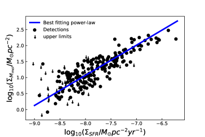
For this sub-sample, the SFR and molecular gas surface densities are related by the following formula;
| (2) |
which was determined by fitting a power-law (blue line) in hyper-fit111This same code has been used to determine all the best fits in this paper. (Robotham & Obreschkow, 2015) to the galaxies with H2 detections. Using equation 2, we obtain molecular gas masses from SFRs for the galaxies where a CO detection is not available. For two of the galaxies in our sample, we do not have SFRs or H2 detections (GASS123007 and GASS38198). For these, we determine the molecular gas mass by assuming that their Hi-to-H2 mass ratio is the average value observed in our sample (i.e., 20%). As H2 contributes very little to both and , these assumptions do not affect our results.
3.2 Specific Angular Momentum of the Baryons
To calculate the baryonic specific AM of the disc () we take the mass-weighted average of the specific AM of each component; stars, Hi and molecular gas, as follows:
| (3) |
where , and are the specific AM of the disc stars, molecular gas and Hi, respectively. We use the values of that are available from Paper 1.
We assume that is equal to . This is because it has been shown in works such as Bigiel & Blitz (2012) and Smith et al. (2016) that the surface density profile of the H2 follows closely that of the stars. The specific AM is primarily set by the surface mass density distribution (assuming that the rotation curves are similar for both components), so it follows that the specific AM of the H2 is the same as the stars.
To determine from spatially unresolved data, we proceed as follows. Firstly, we assume the Hi surface density profile () to be universal for all galaxies. This was shown to be a good approximation for the sample in Wang et al. (2016) when radii were normalised by the Hi diameter. To determine the Hi diameter we use the intrinsically tight Hi mass to size relation from Wang et al. (2016):
| (4) |
where is the diameter of the Hi disc measured at a surface density of . We tested the reliability of this approach by also allowing for a variation in diameter consistent with 1 above and below the relation. Accounting for the scatter in the Hi mass-diameter relation changes by a mean difference of dex. The profiles from Wang et al. (2016) are only given out to , (where ), which for the majority of our galaxies (92% of the sample) is less than the extent used to estimate (i.e., ). For consistency with all other quantities is also calculated within . To do so, we linearly extrapolate the universal profile (in log-log space). This extrapolation slightly increases the value of (less than 0.03 dex). Conversely, for the 46 galaxies, where , is reduced by an average of 0.02 dex up to a maximum of 0.15 dex, when compared to calculated within .
Lastly, we assume that the velocity profile is constant for all radii and given by the width of the Hi emission line. This is the same assumption made in Paper 1 for calculating stellar specific AM. This assumption was tested in Paper 1 by comparing constant velocity profiles to the template rotation curves in Catinella et al. (2006), where we showed that the most extreme case of low-mass dwarf galaxies (i.e. ), had a maximum systematic offset in j of dex, while high-mass galaxies had less discrepancy ( dex). Therefore, this assumption only introduces minor systematic effects which do not impact our result (for more details see Paper 1). We emphasise that, despite using a constant velocity profile, our approach does not rely on the approximation of (Romanowsky & Fall, 2012), and instead estimates j by directly integrating the AM profile obtained from the surface density profiles of each baryonic component. We found this to be a more accurate way to determine AM, as the Romanowsky & Fall (2012) approximation can overestimate a galaxies AM by up to 25% at low masses (e.g., Obreschkow & Glazebrook, 2014; Bouché et al., 2021).
Once all of these assumptions are combined, we obtain . When comparing and , on average is roughly twice the value of , although there is a considerable spread ( dex). Note that this factor 2 was also found in things (Obreschkow & Glazebrook, 2014) using resolved Hi kinematic maps.
We reiterate that although we have outlined many assumptions in this subsection, these choices are not likely to affect our results. Although we assume that stars and gas share the same rotation curve (by using Hi line widths to calculate AM for both), this does not impact our results. Stellar rotation curves rise more slowly than cold gas ones due to asymmetric drift, so our estimates of may be slightly overestimated. However, would not change considerably if was altered slightly. In addition, assumptions made when calculating were robustly tested in Paper 1. As mentioned above, the assumptions involving have been tested, and even if these assumptions are altered, they do not affect the result significantly. In addition, the molecular mass is only a small component of our galaxies, such that excluding molecular material, only alters by 0.02 dex and by 0.01 dex on average. In summary, the typical uncertainty on our estimate of is 0.14 dex, which is dominated by the assumptions made on . This is comparable to the statistical error on , i.e., 0.11 dex.
4 Results
In this section, we investigate the connection between , and atomic gas fractions.
4.1 Baryonic Fall Relation
As a first step, in Figure 2 we show the baryonic Fall relation for galaxies in xGASS.

The left panel shows the baryonic mass and specific AM for just the disc component ( and ), while on the right we show the total (i.e., disc and bulge component; and ). Although the majority of the paper will focus on just the disc components, we also show the right panel to compare with previous works. The best-fit linear relation to our data is shown as a thin black line, with 1 scatter shown by the dashed lines. The blue line shows the baryonic Fall relation found by Murugeshan et al. (2020) and the magenta line is from Mancera Piña et al. (2021a), which both agree well with the best-fitting relation to our work. This is not a trivial result given the difference in samples and techniques used to determine this relation. Therefore, the agreement with previous work gives us confidence that our approach is solid and we can move forward in our analysis.
As for previous works, we suggest caution when interpreting the slopes of the baryonic Fall relation at face value, as our sample is not selected by baryonic mass. xGASS is selected to only include galaxies with stellar masses greater than with an oversampling at the high stellar mass end to increase statistics (as shown in Paper 1 this distribution is conserved for our sub-sample). As such, the distribution in baryonic mass of our sample is not representative, with a deficiency of galaxies at lower baryonic masses. Below a baryonic mass of approximately , at fixed baryonic mass, our sample will preferentially miss galaxies at high gas fractions, whose stellar mass lies below the cut of . In addition, we know from the results of works such as Mancera Piña et al. (2021a, see also Paper 1) that galaxies with higher gas fractions also have higher . Therefore, we would expect the Fall relation to be shallower for a sample that is uniformly distributed in baryonic mass. This echoes the conclusions of Paper 1, which found that the sample used to determine a Fall relation will affect the slope obtained.
4.2 Hi content predicted from local stability
O16 developed a formalism to look at the connection between specific baryonic AM, baryonic mass and atomic gas. This resulted in a dimensionless effective stability parameter q;
| (5) |
where is the baryonic specific AM of the disc component, is the one-dimensional velocity dispersion of Hi, G is the gravitational constant and is the baryonic mass of the disc component. We use and as defined in sections 3.1 and 3.2 respectively. is assumed to be a constant 10 km s-1, which is set by the temperature of the warm neutral medium (following the assumption of O16). For a flat exponential disc, the q parameter relates to the expected fraction of atomic gas via;
| (6) |
Here the fraction of atomic gas is defined as the fraction of disc baryonic mass in neutral atomic hydrogen and helium;
| (7) |
This stability model assumes that any atomic gas that is unstable (following the Toomre 1964 stability parameter Q) will collapse to form stars. As a consequence, if , then the galaxy is over-saturated in Hi and is bound to form stars quickly (i.e., within a giant molecular clouds free-fall time). However, in the opposite case () a galaxy will remain stable, with no self-regulating processes to alter its atomic gas fraction. Therefore, the O16 relation (equation 6) can be thought of as an upper limit of the amount of atomic gas that a galaxy can hold (for further details of the models assumptions see O16).

Figure 3 shows the relationship between the q stability parameter and . We compare our sample (grey) to the data presented in O16 (coloured points) and their model (black line). The binned median of our data (thick blue line) shows good agreement with the theoretical relation shown in black, however, our data show a larger scatter. For our data the median 16th to 84th percentile is 0.52 dex, whereas it is 0.27 dex for the original O16 data. This result does not depend on the method used to determine , as only weakly depends on the molecular gas mass, and is mostly constrained by the Hi mass. The significant scatter observed for xGASS is an important result, as previous work have used the small observed scatter in the relation to support a scenario in which is the primary galaxy property physically connected to gas fraction (e.g., Obreschkow et al., 2016; Lutz et al., 2018; Murugeshan et al., 2019). Instead, for our sample, the relation shows a spread comparable to that of the well-known relation between gas fraction and colour (median 16th to 84th percentile 0.49 dex).
As mentioned above, the O16 model predicts that galaxies will not lie above the relation for long, as their Hi gas will be unstable and collapse to form stars. O16 expect most galaxies to lie within 40% of the analytical relation given the approximate uncertainties of the model, with only 6 out of their 105 galaxies lying above this point. In our data, above this limit, we have roughly double the fraction (61/559) than found in O16. To understand if this is simply due to issues with the data, we analysed the 61 outlier galaxies via the Tully-Fisher relation (Tully & Fisher, 1977) and found that only 11 of them appear to have underestimated rotational velocities. Therefore, as this issue does not affect the rest of the population scattering above the theoretical line, it suggests that the larger scatter compared to what is seen in O16 is not due to data quality but intrinsic to our sample.
Previous works have shown that the down-ward scatter of the relation can be due to environmental effects removing the gas from the disc without affecting the stability parameter (e.g. Li et al., 2020; Cortese et al., 2021). If we divide our sample into central (N=432) and satellites (N=122) according to the classification from the Yang et al. (2007) group catalogue, we find that even in our sample, at fixed q, satellites show a lower (0.2 dex on average) than central galaxies. This is intriguing, as xGASS includes less extreme density environments than the Virgo cluster analysed in Li et al. (2020). However, even if we focus on central galaxies alone, the scatter in the relation remains substantial, with a median 16th to 84th percentile of 0.42 dex. This means that the large spread in at fixed q does not only trace environmentally-driven gas stripping.
To further understand the physical origin for this large scatter, we tested many potential galaxy parameters that could be correlated with the vertical offset from the theoretical - q relation, defined as follows;
| (8) |
Namely, we investigated: the bulge-to-total mass ratio (B/T), Sersic index, Hi depletion time (/SFR), baryonic mass (), specific SFR and the offset of galaxies from the star-forming main sequence (MS, see Section 2). These parameters were chosen as they either related to morphology (which has been shown to relate to the scatter of the Fall relation; Romanowsky & Fall 2012; Cortese et al. 2016; Hardwick et al. 2022) or are an aspect of the model that we wanted to make sure was being encapsulated properly. We use the Spearman rank correlation coefficients () to quantify the correlation between each quantity and the offset from the theoretical line, as shown in Table 1 in descending order of correlation. We chose to use Spearman rank to measure the correlation as it does not make any assumptions on the type of correlation between the two quantities.
| Parameter | Spearman Correlation Coefficient |
|---|---|
| MS | |
| specific SFR | |
| Baryonic Mass | |
| Hi Depletion time | |
| B/T | |
| Sersic index |
The strongest correlation with is MS, which is known to be strongly linked to a galaxy’s atomic gas reservoir (e.g. Catinella et al., 2018; Janowiecki et al., 2020; Saintonge & Catinella, 2022). There is also a non-negligible correlation between and . This implies that the plane may not provide the best representation for the link between AM and gas content in our data, and that xGASS galaxies may be better described by a model with different dependencies on and . Therefore, the next step is to use a more empirical approach and look for the best way parameterise the correlation between , and .
4.3 Empirical 3D fit to j - M - fatm
By fitting a plane to specific AM, mass and gas fraction, we aim to quantify what functional form better describes our data and how this differs from the O16 model. We chose to fit two planes; one for the baryonic parameters (, and ) and one for stellar parameters (, and ). Although the majority of this work is focused on baryonic parameters, we also chose to investigate this parameter space using just stellar properties as, a) the stellar parameters have been more extensively studied in the literature (e.g., Mancera Piña et al., 2021b; Hardwick et al., 2022) and b) they allow us to check if any of our conclusions are affected by the assumptions made to estimate the baryonic AM. We fit these 3-dimensional planes using the following formula;
| (9) |
where is either disc baryons or stars (). The best-fitting parameters to equation 9 are shown in Table 2.
| This work | stellar | ||||
|---|---|---|---|---|---|
| baryonic | |||||
| O16 model | baryonic | 1 | 0.89 | -6.72 |
For comparison, when the O16 relation is converted into this formalism, the free parameters of equation 9 would be , and km s-1 km s-1 . Table 2 shows that, as hinted in the previous section, the best-fit parameters to our data are significantly different from those predicted by the O16 model. In particular, there is a slightly weaker dependence on the mass () term, and a significantly weaker dependence on the gas fraction () term, which is approximately half that expected by the O16 model. The empirical fit also has a smaller scatter (0.15 dex vertical scatter in , compared to 0.23 dex vertical scatter observed for our data in the O16 projection).
We obtain very similar results to that of Mancera Piña et al. (2021b) who, as mentioned in Section 1, also fit a 3D plane to baryonic AM, mass and atomic gas fraction. The coefficients of our planes are consistent within 3, despite their work focusing on a small sample (N = 157) of gas-rich disc galaxies. The only major difference between the results of this work and that of Mancera Piña et al. (2021b) was that they are very confident in their error analysis and quoted intrinsic scatter of their plane (which did not include measurement errors). Conversely, as we believe that we are not able to estimate proper errors for each individual galaxy in our sample, we chose to give which includes both measurement and intrinsic scatter of the plane. If we assume that our error estimates are correct, we find enticing evidence for nearly zero intrinsic scatter in our plane, i.e., a plane much tighter than what found in Mancera Piña et al. (2021b). However, as mentioned above, these errors are only approximations and we advice caution in over-interpreting this result.

Figure 4 shows the stellar (panel a) and baryonic (panel b) relations in the mass - AM plane. Projections of the best-fitting 3D relations from Table 2 are shown for fixed gas fractions as coloured lines. To easily compare, points are colour coded in the same way (i.e., by their gas fractions). The 2D best-fit Fall relation is shown as a thin black line (with the vertical 1 scatter as black dashed lines).

For comparison, Figure 5 shows the same baryonic Fall relation presented in 4b, but this time the lines of constant gas fraction correspond to the prediction from the O16 model. The comparison between Figure 4b and 5 helps visualising the differences between the O16 model and the best-fit empirical relation. Specifically, as already mentioned, the empirical relation has a weaker dependence on atomic gas fraction,which can be seen by the larger separation of the lines of constant gas fraction in Figure 5. The weaker dependence on baryonic mass is also evident, as the lines at fixed gas fraction have a shallower slope than the O16 projection.
A possible issue with the results presented so far is that xGASS was selected to have a nearly flat stellar distribution (Catinella et al., 2018; Hardwick et al., 2022), and the oversampling of high mass galaxies may affect our best-fitting results. To test this, we also fit the empirical relation including weights for each galaxy. Following Catinella et al. (2018), these weights were calculated to recover the distribution of a volume-limited sample using the local stellar mass function as defined in Baldry et al. (2012). We find that, even after including the weights, our best-fit parameters are within error of the values presented in Table 2. Therefore, for simplicity, we only present the values obtained without the weights.
Interestingly, the scatter of the empirical relation still shows a weak correlation with MS, with a Spearman rank correlation coefficient of . Thus, it is worth exploring whether such residual dependence needs to be included in our fit. We trialled fitting a 4D plane, with MS as a fourth parameter and found that the dependence on and was largely unchanged when compared to the 3D plane, with a very small dependence () given to the MS term. In addition to this, the standard deviation between the 4D and 3D fits was unchanged. We conclude that any third-order dependence on MS is negligible or at least within the scatter of the 3D fit presented here.

The choice to use a planar fit for our empirical relation was motivated by the aim of keeping a similar approach to the one adopted by O16, but we also tested for non-linear trends in the residuals of the empirical fit, to see if this choice was sensible. There is a slight curvature in the residuals, when binned in , as is shown in Figure 6. This is a potential indication that the 3D planar fit may be too restrictive. However, the curvature is very weak and would likely not change the fit considerably if fit with a curved surface. Therefore, while we cannot exclude a curvature in the plane, our sample size is too small to justify the use of a 3D curved surface to parametrise the , , plane.
5 Discussion
Our work shows that the O16 model provides a good first-order representation for the relation between gas fraction and AM. However, thanks to the larger dynamic range covered by xGASS compared to previous samples, we have been able to highlight where this analytical model breaks down (in a similar way to Mancera Piña et al. 2021b). Specifically, we show that the predicted slope of the baryonic mass - AM relation at fixed gas fraction is shallower than what is predicted by O16, with a significantly weaker dependence on gas fraction. This is most evident in Figure 7, where we directly compare the O16 model and our empirical best-fit relation to our data at fixed gas fraction. In the top row, our data (coloured points) follow a shallower relation than what is predicted by O16 (shaded region), with the largest deviation at lower gas fractions.

It is important to note that our findings are not a by-product of the methodology adopted to estimate . In fact, our main conclusions remain the same if we use stellar quantities alone (see left panel of Figure 4), showing that our results are not driven by assumptions made on or . Furthermore, the difference between the O16 model and our best-fit plane is also evident if we examine galaxies in different gas fraction bins separately (as shown in Figure 7), for which any systematic variation in the shape of the Hi surface density profile should be further reduced (see Wang et al., 2016).
The inability of the O16 model to fully reproduce our data should not come as a surprise. This analytic model makes some simplistic assumptions, such as assuming atomic gas and stars are distinct spatially and galaxies are thin axially symmetric equilibrium discs with perfectly circular orbits, any of which could be causing the discrepancies between the model and our sample.
A similar analytical model has been recently put forward by Romeo (2020), which uses stability arguments to develop scaling relations involving AM. Their model treats each galaxy component (stars, atomic and molecular gas) separately, with each component regulating its own stability, leading to the expression (where denotes either stars, atomic or molecular gas), which is then used to investigate the scaling relation between AM and gas or stellar mass fraction. We tested the prediction of the Romeo (2020) model on our sample focusing on atomic gas fraction, and found that our data disagree with the model. As with the disagreement with O16, our data prefer a model with a weaker dependence on gas fraction than the Romeo (2020) model predicts. This is also consistent with the recent work of Mancera Piña et al. (2021b), who found that the Romeo (2020) model was not able to reproduce their data either.
We can therefore go back and focus on the O16 model. Before proposing any new changes, it is first important to remember that, as discussed in Section 4.2, the O16 model does not predict a best-fitting scaling relation, but more simply identifies the parameter space in the plane in which galaxies with stable Hi discs should exist. Galaxies that have too much Hi to be stable (i.e., lying above the model) will start rapidly forming stars causing the galaxy to drop down onto the model. No such self-regulation is expected below the model, where there is less Hi than can be supported by the stability of the disc. This Hi depletion can be easily achieved by many processes such as environmental processes, outflows, etc. Therefore, galaxies are not necessarily expected to be normally distributed around this model and instead preferentially scatter below the relation. As such a best-fit to a sample of galaxies that obeys the O16 model will most likely be offset below the O16 model. If we assume that processes that cause galaxies to scatter below the relation affect all masses equally, then this best-fit would have the same dependence on and as the O16 model. However, as shown clearly in Figure 4 and 7, the best-fit empirical model has a different slope, implying a weaker dependence on baryonic mass and gas fraction than predicted. We briefly discuss if any processes could cause these changes.
One key assumption made in the O16 model is that galaxies live in isolation. As discussed in Section 4.2, environment plays a role in the scatter around the O16 relation, and can also introduce a mass dependence due to environmental processes being more efficient in low mass galaxies. However, this is unlikely to be the main driver of the deviations, as xGASS does not include galaxies in large cluster environments with the majority of the galaxies in our sample being central/ field galaxies. Even when we do exclude satellite galaxies from our sample, we still see a disparity between these galaxies and the O16 model. Major mergers are also unlikely to be causing this discrepancy, primarily because these are quite rare in the xGASS volume and confused galaxies (including close pairs and merging systems) were excluded from the sample.
The fact that galaxies are not isolated also implies that processes such as smooth gas inflows and outflows (and feedback in general) can play an important role in driving the deviations from the O16 model. The effect of these is quite challenging to predict analytically. However, it is possible that feedback could impact the connection between gas fraction and by affecting one or more of the key physical quantities at the basis of the O16 model: i.e., gas content, AM and velocity dispersion.
Lastly, the modelling of the 3D structure of galaxies itself most likely harbours some of the limitations of the model. Local instabilities caused by spiral arms (e.g. Goldreich & Lynden-Bell, 1965; Toomre, 1977; Dobbs & Baba, 2014), as well as the presence of a significant photometric bulge component in more than half of xGASS galaxies, makes our sample clearly deviating from the simple assumption of axis-symmetric thin discs made in the O16 model. All this can easily make the assumption of constant Hi velocity dispersion incorrect. In fact, it has been shown that the Hi velocity dispersion radial profiles of nearby galaxies are not constant and that even the average value across the disc varies from galaxy to galaxy (e.g. Bacchini et al., 2019). In addition, if the change in correlates with either baryonic mass or gas fraction, it may be even easier to reconcile the tension between our data and the O16 model. Unfortunately, observational constraints on the variation of with galaxy properties are still missing. However, this is an intriguing scenario which could address the issues emerged in this analysis without major changes to the overall physical framework of the O16 model.
Admittedly, what we discussed so far is primarily speculation, but it is likely that more than one of the issues described above are driving the differences between O16 and our data. This is because, as illustrated in Figure 7, the tension between our data and the O16 model are present even in the high gas fraction, disc-dominated regime for which this model has been calibrated, and then extends to more gas-poor disc plus bulge systems for which the assumptions of the O16 model naturally break. This highlights how understanding the physical drivers for the correlation between mass, AM and gas fraction is clearly a complex and multi-dimensional problem. The next step towards the solution of this problem may no longer come from a more elaborate analytical model, but instead from investigating this problem in a self-consistent cosmological framework. This will be our next step towards fully understanding the connection between AM and gas fraction and the origin of the weaker-than-expected correlation between these properties observed in the xGASS sample.
6 Summary and Conclusions
In this work, we have used a representative sample of galaxies in the local Universe with to investigate the connection between baryonic mass, specific AM and atomic gas fraction. We primarily focus on the comparison of our data with the predictions of the O16 stability model.
We show that, as a first-order approximation, the O16 model agrees well with our sample. However, when a full analysis is conducted, we see that our data show a slightly weaker dependence on baryonic mass, and half the dependence on atomic gas fraction than what suggested by the O16 model. This implies that the physical connection between AM and gas fraction may be weaker than claimed in previous works, and suggests that some of the assumptions made in the O16 model are not a good representation of the diversity of our data. While we speculate that part of this tension may be due to galaxy-to-galaxy variations, it is likely that multiple factors (e.g., internal galaxy properties and environmental effects) are simultaneously responsible for the weaker correlation between AM and gas fraction. In future work, we plan to further expand this analysis by performing a detailed study of cosmological simulations with the aim of gaining more insights into the exact cause of the discrepancy between our data and the O16 model.
Acknowledgements
We thank the anonymous referee for their comments which improved the clarity of our manuscript. JAH and LC acknowledge support from the Australian Research Council (FT180100066). Parts of this research were conducted by the Australian Research Council Centre of Excellence for All Sky Astrophysics in 3 Dimensions (ASTRO 3D), through project number CE170100013. DO is a recipient of an Australian Research Council Future Fellowship (FT190100083), funded by the Australian Government.
Data Availability
The data used in this work are publicly available at xgass.icrar.org/data.html.
References
- Accurso et al. (2017) Accurso G., et al., 2017, Monthly Notices of the Royal Astronomical Society
- Adelman-McCarthy et al. (2008) Adelman-McCarthy J. K., et al., 2008, The Astrophysical Journal Supplement Series, 175, 297
- Bacchini et al. (2019) Bacchini C., Fraternali F., Iorio G., Pezzulli G., 2019, Astronomy and Astrophysics, 622, A64
- Baldry et al. (2012) Baldry I. K., et al., 2012, Monthly Notices of the Royal Astronomical Society, 421, 621
- Bernardi et al. (2003) Bernardi M., et al., 2003, The Astronomical Journal, 125, 1849
- Bigiel & Blitz (2012) Bigiel F., Blitz L., 2012, The Astrophysical Journal, 756, 183
- Boissier & Prantzos (2000) Boissier S., Prantzos N., 2000, Monthly Notices of the Royal Astronomical Society, 312, 398
- Bouché et al. (2021) Bouché N. F., et al., 2021, A&A, 654, A49
- Catinella et al. (2006) Catinella B., Giovanelli R., Haynes M. P., 2006, The Astrophysical Journal, 640, 751
- Catinella et al. (2010) Catinella B., et al., 2010, Monthly Notices of the Royal Astronomical Society, 403, 683
- Catinella et al. (2018) Catinella B., et al., 2018, Monthly Notices of the Royal Astronomical Society, 476, 875
- Cook et al. (2019) Cook R. H. W., Cortese L., Catinella B., Robotham A., 2019, Monthly Notices of the Royal Astronomical Society, 490, 4060
- Cortese et al. (2016) Cortese L., et al., 2016, Monthly Notices of the Royal Astronomical Society, 463, 170
- Cortese et al. (2021) Cortese L., Catinella B., Smith R., 2021, Publications of the Astronomical Society of Australia, 38, e035
- Courteau et al. (2007) Courteau S., Dutton A. A., van den Bosch F. C., MacArthur L. A., Dekel A., McIntosh D. H., Dale D. A., 2007, The Astrophysical Journal, 671, 203
- Dobbs & Baba (2014) Dobbs C., Baba J., 2014, Publications of the Astronomical Society of Australia, 31, e035
- Džudžar et al. (2019) Džudžar R., et al., 2019, Monthly Notices of the Royal Astronomical Society, 483, 5409
- Fall (1983) Fall S. M., 1983, in Internal Kinematics and Dynamics of Galaxies. pp 391–398, http://adsabs.harvard.edu/abs/1983IAUS..100..391F
- Goldreich & Lynden-Bell (1965) Goldreich P., Lynden-Bell D., 1965, Monthly Notices of the Royal Astronomical Society, 130, 125
- Hardwick et al. (2022) Hardwick J. A., Cortese L., Obreschkow D., Catinella B., Cook R. H. W., 2022, Monthly Notices of the Royal Astronomical Society, 509, 3751
- Huang et al. (2012) Huang S., Haynes M. P., Giovanelli R., Brinchmann J., 2012, The Astrophysical Journal, 756, 113
- Janowiecki et al. (2017) Janowiecki S., Catinella B., Cortese L., Saintonge A., Brown T., Wang J., 2017, Monthly Notices of the Royal Astronomical Society, 466, 4795
- Janowiecki et al. (2020) Janowiecki S., Catinella B., Cortese L., Saintonge A., Wang J., 2020, Monthly Notices of the Royal Astronomical Society, 493, 1982
- Kennicutt (1989) Kennicutt Robert C. J., 1989, ApJ, 344, 685
- Kurapati et al. (2021) Kurapati S., Chengalur J. N., Verheijen M. A. W., 2021, Monthly Notices of the Royal Astronomical Society, 507, 565
- Lagos et al. (2017) Lagos C. d. P., Theuns T., Stevens A. R. H., Cortese L., Padilla N. D., Davis T. A., Contreras S., Croton D., 2017, Monthly Notices of the Royal Astronomical Society, 464, 3850
- Li et al. (2020) Li J., Obreschkow D., Lagos C., Cortese L., Welker C., Džudžar R., 2020, Monthly Notices of the Royal Astronomical Society, 493, 5024
- Lutz et al. (2018) Lutz K. A., et al., 2018, Monthly Notices of the Royal Astronomical Society, 476, 3744
- Mancera Piña et al. (2021a) Mancera Piña P. E., Posti L., Fraternali F., Adams E. A. K., Oosterloo T., 2021a, Astronomy & Astrophysics, 647, A76
- Mancera Piña et al. (2021b) Mancera Piña P. E., Posti L., Pezzulli G., Fraternali F., Fall S. M., Oosterloo T., Adams E. A. K., 2021b, Astronomy & Astrophysics, 651, L15
- Martin et al. (2005) Martin D. C., et al., 2005, The Astrophysical Journal, 619, L1
- Mo et al. (1998) Mo H. J., Mao S., White S. D. M., 1998, Monthly Notices of the Royal Astronomical Society, 295, 319
- Murugeshan et al. (2019) Murugeshan C., Kilborn V., Obreschkow D., Glazebrook K., Lutz K., Džudžar R., Dénes H., 2019, Monthly Notices of the Royal Astronomical Society, 483, 2398
- Murugeshan et al. (2020) Murugeshan C., Kilborn V., Jarrett T., Wong O. I., Obreschkow D., Glazebrook K., Cluver M. E., Fluke C. J., 2020, Monthly Notices of the Royal Astronomical Society, 496, 2516
- Murugeshan et al. (2021) Murugeshan C., et al., 2021, Monthly Notices of the Royal Astronomical Society, 507, 2949
- Obreschkow & Glazebrook (2014) Obreschkow D., Glazebrook K., 2014, The Astrophysical Journal, 784, 26
- Obreschkow et al. (2016) Obreschkow D., Glazebrook K., Kilborn V., Lutz K., 2016, The Astrophysical Journal Letters, 824, L26
- Robotham & Obreschkow (2015) Robotham A. S. G., Obreschkow D., 2015, Publications of the Astronomical Society of Australia, 32, e033
- Romanowsky & Fall (2012) Romanowsky A. J., Fall S. M., 2012, The Astrophysical Journal Supplement Series, 203, 17
- Romeo (2020) Romeo A. B., 2020, Monthly Notices of the Royal Astronomical Society, 491, 4843
- Saintonge & Catinella (2022) Saintonge A., Catinella B., 2022, Annual Review of Astronomy and Astrophysics, 60
- Saintonge et al. (2011) Saintonge A., et al., 2011, Monthly Notices of the Royal Astronomical Society, 415, 32
- Saintonge et al. (2017) Saintonge A., et al., 2017, The Astrophysical Journal Supplement Series, 233, 22
- Schmidt (1959) Schmidt M., 1959, ApJ, 129, 243
- Smith et al. (2016) Smith M. W. L., et al., 2016, Monthly Notices of the Royal Astronomical Society, 462, 331
- Stevens et al. (2018) Stevens A. R. H., Lagos C. d. P., Obreschkow D., Sinha M., 2018, Monthly Notices of the Royal Astronomical Society, 481, 5543
- Stevens et al. (2019) Stevens A. R. H., et al., 2019, Monthly Notices of the Royal Astronomical Society, 483, 5334
- Toomre (1964) Toomre A., 1964, The Astrophysical Journal, 139, 1217
- Toomre (1977) Toomre A., 1977, In: Annual review of astronomy and astrophysics. Volume 15. (A78-16576 04-90) Palo Alto, Calif., Annual Reviews, Inc., 1977, p. 437-478. NSF-supported research., 15, 437
- Tully & Fisher (1977) Tully R. B., Fisher J. R., 1977, Astronomy and Astrophysics, 54, 661
- Wang et al. (2016) Wang J., Koribalski B. S., Serra P., van der Hulst T., Roychowdhury S., Kamphuis P., Chengalur J. N., 2016, Monthly Notices of the Royal Astronomical Society, 460, 2143
- Wang et al. (2018) Wang L., et al., 2018, The Astrophysical Journal, 868, 93
- Wang et al. (2019) Wang L., et al., 2019, Monthly Notices of the Royal Astronomical Society, 482, 5477
- Wright et al. (2010) Wright E. L., et al., 2010, The Astronomical Journal, 140, 1868
- Yang et al. (2007) Yang X., Mo H. J., van den Bosch F. C., Pasquali A., Li C., Barden M., 2007, The Astrophysical Journal, 671, 153