This paper was converted on www.awesomepapers.org from LaTeX by an anonymous user.
Want to know more? Visit the Converter page.

aainstitutetext: Helmholtz-Zentrum Dresden-Rossendorf, Bautzner Landstraße 400, 01328 Dresden, Germanyccinstitutetext: Dipartimento di Fisica e Astronomia “Augusto Righi”, Università di Bologna, Via Irnerio 46, I-40126 Bologna, Italyddinstitutetext: INFN, Sezione di Bologna, Via Irnerio 46, I-40126 Bologna, Italyeeinstitutetext: Dipartimento di Scienze Fisiche, Informatiche e Matematiche, Università degli Studi di Modena e Reggio Emilia, Via Campi 213/A, I-41125 Modena, Italyffinstitutetext: Instituto de Física y Matemáticas Universidad Michoacana de San Nicolás de Hidalgo Edificio C-3, Apdo. Postal 2-82 C.P. 58040, Morelia, Michoacán, México

Worldline master formulas for the dressed electron propagator, part 2: On-shell amplitudes

N. Ahmadiniaz f    V. M. Banda Guzmán c,d    F. Bastianelli e,d    O. Corradini f    J.P. Edwards f    and C. Schubert [email protected] [email protected] [email protected] [email protected] [email protected] [email protected]
Abstract

In the first part of this series, we employed the second-order formalism and the “symbol” map to construct a particle path-integral representation of the electron propagator in a background electromagnetic field, suitable for open fermion-line calculations. Its main advantages are the avoidance of long products of Dirac matrices, and its ability to unify whole sets of Feynman diagrams related by permutation of photon legs along the fermion lines. We obtained a Bern-Kosower type master formula for the fermion propagator, dressed with NN photons, in terms of the “NN-photon kernel,” where this kernel appears also in “subleading” terms involving only N1N-1 of the NN photons.

In this sequel, we focus on the application of the formalism to the calculation of on-shell amplitudes and cross sections. Universal formulas are obtained for the fully polarised matrix elements of the fermion propagator dressed with an arbitrary number of photons, as well as for the corresponding spin-averaged cross sections. A major simplification of the on-shell case is that the subleading terms drop out, but we also pinpoint other, less obvious simplifications.

We use integration by parts to achieve manifest transversality of these amplitudes at the integrand level and exploit this property using the spinor helicity technique. We give a simple proof of the vanishing of the matrix element for “all ++” photon helicities in the massless case, and find a novel relation between the scalar and spinor spin-averaged cross sections in the massive case. Testing the formalism on the standard linear Compton scattering process, we find that it reproduces the known results with remarkable efficiency. Further applications and generalisations are pointed out.

1 Introduction

In the first part of this series 130 , simply to be called ‘I’ in the following, we developed a novel path-integral representation of the electron propagator in an external electromagnetic field suitable for practical calculations in the worldline approach to QED feynman:pr80 ; feynman:pr84 ; polyakovbook ; strassler1 ; strassler2 ; 5 ; 15 ; 41 ; UsRep , in particular for tree-level amplitudes involving multiple photons and related quantities. In contrast to the standard first-order Dirac formalism, it is based on the less-known but equivalent second order fermion approach to spinor QED feygel ; hostler ; berdun ; morgan . Let us briefly retrace the main steps of this derivation, referring the reader to I for the details.

1.1 Short review of the formalism

The starting point in the second-order formalism is the following factorisation of the xx-space Dirac propagator Sxx[A]S^{x^{\prime}x}[A] in a Maxwell background (we suppress spin indices for brevity),

Sxx[A]\displaystyle S^{x^{\prime}x}[A] =\displaystyle= [m+i]Kxx[A],\displaystyle\bigl{[}m+i\not{D}^{\prime}\bigr{]}K^{x^{\prime}x}[A]\,, (1)

where =γμDμ\not{D}^{\prime}=\gamma^{\mu}D^{\prime}_{\mu}, Dμ=μ+ieAμ(x)D_{\mu}^{\prime}=\partial_{\mu}^{\prime}+ieA_{\mu}(x^{\prime}) is the covariant derivative and we introduced the matrix elements111See appendix A for our conventions.

Kxx[A]\displaystyle K^{x^{\prime}x}[A] \displaystyle\equiv x|[m2+π^μπ^μ+i2eγμγνFμν(x^)]1|x\displaystyle\langle x^{\prime}\big{|}\bigl{[}m^{2}+\hskip 3.00003pt\widehat{\pi}\hskip 3.99994pt^{\mu}\hskip 3.00003pt\widehat{\pi}\hskip 3.99994pt_{\mu}+{i\over 2}\,e\gamma^{\mu}\gamma^{\nu}F_{\mu\nu}(\hskip 3.00003pt\widehat{x}\hskip 3.99994pt)\bigr{]}^{-1}\big{|}x\rangle (2)

where π^μ=p^μ+eAμ(x^)\hskip 3.00003pt\widehat{\pi}\hskip 3.99994pt_{\mu}=\hskip 3.00003pt\widehat{p}\hskip 3.99994pt_{\mu}+eA_{\mu}(\hskip 3.00003pt\widehat{x}\hskip 3.99994pt). For this “kernel” function, following fragit , we then derived the following path integral representation:

Kxx[A]\displaystyle K^{x^{\prime}x}[A] =\displaystyle= 0𝑑Tem2Te14(xx)2Tq(0)=0q(T)=0Dqe0T𝑑τ[14q˙2+ieq˙A(x0+q)+iexxTA(x0+q)]\displaystyle\int_{0}^{\infty}dT\,\,{\rm e}^{-m^{2}T}\,{\rm e}^{-{1\over 4}\frac{(x-x^{\prime})^{2}}{T}}\int_{q(0)=0}^{q(T)=0}Dq\,{\rm e}^{-\int_{0}^{T}d\tau\bigl{[}{1\over 4}\dot{q}^{2}+ie\,\dot{q}\cdot A(x_{0}+q)+ie\frac{x^{\prime}-x}{T}\cdot A(x_{0}+q)\bigr{]}} (3)
×2D2symb1ψ(0)+ψ(T)=0Dψe0Tdτ[12ψμψ˙μie(ψ+η)μFμν(x0+q)(ψ+η)ν].\displaystyle\times 2^{-\frac{D}{2}}{\rm symb}^{-1}\int_{\psi(0)+\psi(T)=0}D\psi\,\,{\rm e}^{-\int_{0}^{T}d\tau\,\bigl{[}{1\over 2}\psi_{\mu}\dot{\psi}^{\mu}-ie(\psi+\eta)^{\mu}F_{\mu\nu}(x_{0}+q)(\psi+\eta)^{\nu}\bigl{]}}\,.

Here x0=x+τT(xx)x_{0}=x+\frac{\tau}{T}(x^{\prime}-x) is the straight-line path between the endpoints, ημ\eta^{\mu} is an external Grassmann Lorentz vector, and the inverse of the “symbol map” symb converts products of η\eta’s into fully antisymmetrised products of Dirac matrices,

symb(γ[α1α2αn])(i2)nηα1ηα2ηαn.\displaystyle{\rm symb}\bigl{(}\gamma^{[\alpha_{1}\alpha_{2}\cdots\alpha_{n}]}\bigr{)}\equiv(-i\sqrt{2})^{n}\eta^{\alpha_{1}}\eta^{\alpha_{2}}\ldots\eta^{\alpha_{n}}\,. (4)

When working in four dimensions, this reduces to the three cases

symb1(1)\displaystyle{\rm symb}^{-1}(1) =\displaystyle= 1l,\displaystyle{\mathchoice{\rm 1\mskip-4.0mul}{\rm 1\mskip-4.0mul}{\rm 1\mskip-4.5mul}{\rm 1\mskip-5.0mul}}\,, (5)
symb1(ηα1ηα2)\displaystyle{\rm symb}^{-1}(\eta^{\alpha_{1}}\eta^{\alpha_{2}}) =\displaystyle= 14[γα1,γα2],\displaystyle-\frac{1}{4}[\gamma^{\alpha_{1}},\gamma^{\alpha_{2}}]\,, (6)
symb1(ηα1ηα2ηα3ηα4)\displaystyle{\rm symb}^{-1}(\eta^{\alpha_{1}}\eta^{\alpha_{2}}\eta^{\alpha_{3}}\eta^{\alpha_{4}}) =\displaystyle= i4εα1α2α3α4γ5.\displaystyle-\frac{i}{4}\varepsilon^{\alpha_{1}\alpha_{2}\alpha_{3}\alpha_{4}}\gamma_{5}\,. (7)

We then performed the usual projection onto an NN-photon background of fixed momenta and polarisations, and used Gaussian integration on both the orbital path integral, Dq(τ)\int Dq(\tau), and spin path integral, Dψ(τ)\int D\psi(\tau), to derive Bern-Kosower type master formulas for the NN-photon kernel KK both in configuration and in momentum space. We also showed a convenient way to decompose these amplitudes into contributions with a fixed number of orbital and spin interactions, which we refer to as a spin-orbit decomposition.

As in I, in our applications here we will focus entirely on momentum-space amplitudes. Fourier transforming the starting identity (1) to momentum space, and projecting it onto the NN-photon sector, it turns into

SNpp[k1,ε1;;kN,εN]\displaystyle S_{N}^{p^{\prime}p}[k_{1},\varepsilon_{1};\ldots;k_{N},\varepsilon_{N}] =\displaystyle= (+m)KNpp[k1,ε1;;kN,εN]\displaystyle({\not{p}^{\prime}}+m)K_{N}^{p^{\prime}p}[k_{1},\varepsilon_{1};\ldots;k_{N},\varepsilon_{N}] (8)
ei=1Nε̸iK(N1)p+ki,p[k1,ε1;;k^i,ε^i;;kN,εN].\displaystyle-e\sum_{i=1}^{N}{\not{\varepsilon}_{i}}K_{(N-1)}^{p^{\prime}+k_{i},p}[k_{1},\varepsilon_{1};\ldots;\hat{k}_{i},\hat{\varepsilon}_{i};\ldots;k_{N},\varepsilon_{N}]\,.

Here in the second term the ‘hat’ on εi\varepsilon_{i} and kik_{i} means omission. The terms involving K(N1)K_{(N-1)} are called “subleading” and arise because one of the NN photons could be taken from the AμA_{\mu} appearing in the covariant derivative in the factor [m+i]\bigl{[}m+i\not{D}^{\prime}\bigr{]} in (1). An important advantage of the “worldline representation” is that it automatically takes care of the permutations over the NN photons, and thus avoids the break-up of the amplitude into individual Feynman diagrams. This may not seem very relevant at the tree-level, but becomes an important issue when tree-level amplitudes are used for the construction of multiloop amplitudes by sewing 15 ; 41 ; 100 .

1.2 The on-shell case

In I our focus was on the use of the off-shell amplitudes as a building block for loop amplitudes, which we exemplified by a recalculation of the one-loop electron self-energy in an arbitrary gauge and dimension. Now, our objective is to explore the simplifications which can be achieved in the on-shell case, both for the amplitudes themselves as well as for the linear (N=2N=2) and non-linear (N>2N>2) Compton scattering cross sections that can be constructed out of them. Thus our principal object of interest is the on-shell matrix element corresponding to the dressed electron propagator with fixed spins s,ss,s^{\prime}. In its construction we must remember that the second-order representation of the dressed electron propagator still contains the external propagators, which must be removed before going on-shell. Thus the matrix element has to be written as

Nsspp=u¯s(p)(+m)SNpp(+m)us(p),\displaystyle{\cal M}_{Ns^{\prime}s}^{p^{\prime}p}=\bar{u}_{s^{\prime}}(-p^{\prime})(-{\not{p}^{\prime}}+m)S_{N}^{p^{\prime}p}(\not{p}+m)u_{s}(p)\,, (9)

where the spinors satisfy the on-shell relations

u¯s(p)(+m)=0=(+m)us(p).\displaystyle\bar{u}_{s^{\prime}}(-p^{\prime})(-{\not{p}^{\prime}}+m)=0=(\not{p}+m)u_{s}(p)\,. (10)

Thus these zeroes must be cancelled by corresponding poles to get a non-vanishing matrix element, which is the fermionic version of the LSZ theorem. Looking at the decomposition (8), we can see how this works for the leading term: as explained in part I, KNppK_{N}^{p^{\prime}p} is, in the second-order formalism, built from untruncated Feynman diagrams involving only scalar propagators. Thus it contains a factor 1(p2+m2)(p2+m2)\frac{1}{\left(p^{\prime 2}+m^{2}\right)\left(p^{2}+m^{2}\right)}, which led us to the redefinition (I. 5.11),

KNpp\displaystyle K_{N}^{p^{\prime}p} =\displaystyle= (ie)N𝔎Npp(p2+m2)(p2+m2).\displaystyle(-ie)^{N}\frac{\mathfrak{K}_{N}^{p^{\prime}p}}{\left(p^{\prime 2}+m^{2}\right)\left(p^{2}+m^{2}\right)}\,. (11)

Since m2+p2=(+m)(+m)m^{2}+p^{2}=(\not{p}+m)(-\not{p}+m), the cancellation of the poles can then be made explicit:

u¯s(p)(+m)(+m)𝔎Npp(p2+m2)(p2+m2)(+m)us(p)\displaystyle\bar{u}_{s^{\prime}}(-p^{\prime})(-{\not{p}^{\prime}}+m)(\not{p}^{\prime}+m)\frac{\mathfrak{K}_{N}^{p^{\prime}p}}{\left(p^{\prime 2}+m^{2}\right)\left(p^{2}+m^{2}\right)}(\not{p}+m)u_{s}(p)
=u¯s(p)𝔎Npp+mus(p)=u¯s(p)𝔎Npp2mus(p).\displaystyle=\bar{u}_{s^{\prime}}(-p^{\prime})\frac{\mathfrak{K}_{N}^{p^{\prime}p}}{-\not{p}+m}u_{s}(p)=\bar{u}_{s^{\prime}}(-p^{\prime})\frac{\mathfrak{K}_{N}^{p^{\prime}p}}{2m}u_{s}(p)\,. (12)

The same does not work for the subleading terms, K(N1)p+ki,pK_{(N-1)}^{p^{\prime}+k_{i},p}, since in those the pole 1p2+m2\frac{1}{p^{\prime 2}+m^{2}} has been shifted to 1(p+ki)2+m2\frac{1}{(p^{\prime}+k_{i})^{2}+m^{2}}. Thus they can be omitted in the calculation of on-shell matrix elements, and our final formula for the matrix elements of the NN-photon dressed electron propagator becomes

Nsspp\displaystyle{\cal M}_{Ns^{\prime}s}^{p^{\prime}p} =\displaystyle= (ie)N2mu¯s(p)𝔎Nppus(p).\displaystyle\frac{(-ie)^{N}}{2m}\bar{u}_{s^{\prime}}(-p^{\prime})\mathfrak{K}_{N}^{p^{\prime}p}u_{s}(p)\,. (13)

As is clear from (7), in D=4D=4 the Dirac matrix structure of 𝔎Npp\mathfrak{K}_{N}^{p^{\prime}p} is (I 5.11),

𝔎Npp\displaystyle\mathfrak{K}_{N}^{p^{\prime}p} =\displaystyle= AN11+BNαβσαβiCNγ5,\displaystyle A_{N}1\!\!1+B_{N{\alpha\beta}}\sigma^{\alpha\beta}-iC_{N}\gamma_{5}\,, (14)

with σαβ=12[γα,γβ]\sigma^{\alpha\beta}=\frac{1}{2}[\gamma^{\alpha},\gamma^{\beta}]. Moreover, from the spin-orbit decomposition it is clear that ANA_{N} can be split as

AN=ANscal+ANψ,\displaystyle A_{N}=A_{N}^{\rm scal}+A_{N}^{\psi}\,, (15)

where ANscalA_{N}^{\rm scal} is, up to the coupling constant factor, the truncated scalar propagator (see (I.1.2) for its path integral representation),

(ie)NANscal=D^Npp,\displaystyle(-ie)^{N}A_{N}^{\rm scal}=\hskip 3.00003pt\widehat{D}\hskip 3.99994pt_{N}^{p^{\prime}p}\,, (16)

while terms in ANψA_{N}^{\psi} involve the spin interaction at least once.

On-shell matrix elements in QED are guaranteed to be transversal in the photon polarisations, implying that it must be possible to write the amplitude entirely in terms of photon field-strength tensors, defined by

fμν=kμενεμkν.f_{\mu\nu}=k_{\mu}\varepsilon_{\nu}-\varepsilon_{\mu}k_{\nu}\,. (17)

for a photon of momentum kk with polarisation vector ε\varepsilon. Although this fact is even stated in some textbooks on QFT (see, e.g., peskinschroeder-book ), in the standard Feynman diagram approach it is by no means trivial to actually achieve this rewriting explicitly for an arbitrary number of photons (see, e.g., felihu ). Here we will show both for the dressed scalar propagator DNppD_{N}^{p^{\prime}p} as well as for the kernel KNppK_{N}^{p^{\prime}p} of the dressed electron propagator how this manifest transversality can be achieved at the integrand level by a simple integration-by-parts algorithm. We will also develop some useful formulas for the application of the standard spinor helicity technique to expressions where all polarisation vectors are contained in field-strength tensors.

A less obvious simplification concerning the coefficients AN,BNμν,CNA_{N},B_{N{\mu\nu}},C_{N} is that there are useful relations between them whenever both pp and pp^{\prime} are on-shell. We will see that, for D=4D=4 (B~\widetilde{B} is the dual to BB),

AN(m2pp)\displaystyle A_{N}(m^{2}-p\cdot p^{\prime}) =\displaystyle= 2pμBNμνpν\displaystyle 2p^{\mu}B_{N\mu\nu}p^{\prime\nu} (18)
CN(m2+pp)\displaystyle C_{N}(m^{2}+p\cdot p^{\prime}) =\displaystyle= 2pμB~Nμνpν,\displaystyle 2p^{\mu}\widetilde{B}_{N\mu\nu}p^{\prime\nu}\,, (19)

so that in principle the full information on the matrix element is already contained in BNμνB_{N\mu\nu}.

Our goal of obtaining general expressions for the fully polarised matrix elements, valid for any NN without the explicit knowledge of the coefficient functions AN,BNμν,CNA_{N},B_{N{\mu\nu}},C_{N}, made it necessary to dispose of explicit formulas for the Dirac bilinears appearing when (14) is put into (13). To our surprise, we could not find in the literature explicit formulas for those bilinears valid for general pp, pp^{\prime} and arbitrary spin axes. We have therefore derived suitable formulas ourselves, based on an algorithm proposed recently in olpozp (see section 5).

After summing over electron spins, which we are still able to do for arbitrary NN and photon helicity assignments, further simplification is possible, leading to the following very compact representation for the spin-averaged cross sections:

|Npp|2\displaystyle\big{\langle}\big{|}{\cal M}_{N}^{p^{\prime}p}\big{|}^{2}\big{\rangle} =\displaystyle= e2N[|AN|2+2BNαβBNαβ|CN|2].\displaystyle e^{2N}\Bigl{[}\left|A_{N}\right|^{2}+2B_{N}^{\alpha\beta}B_{N{\alpha\beta}}^{\ast}-\left|C_{N}\right|^{2}\Bigr{]}. (20)

We then apply all this machinery to the N=2N=2 case, performing a complete recalculation of the fully polarised matrix elements for Compton scattering, as well as the spin-averaged and the fully unpolarised cross sections, and recover the known results with relatively little effort.

The organisation of part 2 is as follows. Sections 2 - 6 are preparatory: in section 2 we explain the on-shell IBP procedure leading to the “R-representation” of the integrands of the on-shell photon-dressed scalar and electron propagator. Section 3 contains a collection of formulas involving the fixed-helicity field-strength tensors f±μνf^{\pm{\mu\nu}}. As a warm-up, in section 4 we apply the formalism to the scalar QED case, obtaining the N=2N=2 matrix elements and demonstrating the well-known vanishing of the “all +” amplitudes in the massless limit. Section 5 is devoted to the construction of Dirac bilinears, section 6 to the study of the coefficient functions AN,BNμν,CNA_{N},B_{N{\mu\nu}},C_{N}. The central section of this paper is 7, which contains the construction of the fully polarised matrix elements as well as the spin-averaged cross sections, for arbitrary photon number and helicity assignments. Section 8 deals with the “all +” case, which exhibits some further interesting simplifications related to the well-known connections between helicity, self-duality and supersymmetry thooft ; dadda ; brolee ; dufish1 ; dufish2 ; 51 . In section 9 we apply all these developments to the ordinary Compton scattering case. Our conclusions and directions of future work are offered in section 10.

There are four appendices. In appendix A we summarise our conventions; contrary to I, where Euclidean conventions were used throughout, for the computation of on-shell quantities it is, as usual, preferable to Wick rotate from Euclidean to Minkowski space. Apart from changing the metric from (++++)(++++) to (+++)(-+++), this will also induce a factor of (i)(-i) for each propagator and a factor of ii for each vertex. This amounts to a global factor of (i)(-i) for the dressed scalar or spinor propagators DNppD_{N}^{p^{\prime}p} or SNppS_{N}^{p^{\prime}p}, but a factor ii for their truncated versions D^Npp\hskip 3.00003pt\widehat{D}\hskip 3.99994pt_{N}^{p^{\prime}p} and S^Npp\hskip 3.00003pt\widehat{S}\hskip 3.99994pt_{N}^{p^{\prime}p}, defined by

D^Npp\displaystyle\hskip 3.00003pt\widehat{D}\hskip 3.99994pt_{N}^{p^{\prime}p} \displaystyle\equiv (p2+m2)DNpp(p2+m2),\displaystyle\left(p^{\prime 2}+m^{2}\right)D_{N}^{p^{\prime}p}\left(p^{2}+m^{2}\right)\,, (21)
S^Npp\displaystyle\hskip 3.00003pt\widehat{S}\hskip 3.99994pt_{N}^{p^{\prime}p} \displaystyle\equiv (+m)SNpp(+m).\displaystyle(-{\not{p}^{\prime}}+m)S_{N}^{p^{\prime}p}(\not{p}+m)\,. (22)

Thus in Minkowski space we have iscal,Npp=iD^Nppi{\cal M}_{{\rm scal},N}^{p^{\prime}p}=i\hskip 3.00003pt\widehat{D}\hskip 3.99994pt_{N}^{p^{\prime}p} and ispin,Npp=iS^Nppi{\cal M}_{{\rm spin},N}^{p^{\prime}p}=i\hskip 3.00003pt\widehat{S}\hskip 3.99994pt_{N}^{p^{\prime}p}.

In appendix B we provide explicit formulas for the Dirac bilinears of section 5 for the two most standard choices of electron polarisations, projection of the spin on the direction of motion or on the zz-axis in the electron’s rest frame. Appendix C derives recursion formulas for the coefficient functions AN,BNμν,CNA_{N},B_{N{\mu\nu}},C_{N} that provide an alternative algorithm for their determination. Finally some simplifications peculiar to the massless limit are discussed in appendix D.

2 Manifest transversality at the integrand level

An essential feature of the worldline formalism is the option of using integration-by-parts (‘IBP’) strassler1 ; strassler2 ; 41 ; 26 ; 91 to improve on the integrand of parameter integrals before their actual calculation. For the prototypical case, the one-loop NN-photon amplitudes, one can hope to reduce significantly the number of terms in the integrand, to achieve manifest gauge invariance at the integrand level, eliminate spurious UV divergences (for the N=4N=4 case), and realise the unification of the scalar and spinor QED cases through the “Bern-Kosower cycle replacement rule” berkosPRL ; berkosNPB . Although similar manipulations could also be done using Feynman diagrams, they would usually become much more cumbersome as well as harder to find since they do not involve individual Feynman diagrams but rather whole sets of them.

For general NN, two different IBP algorithms have already been developed: “symmetric IBP” 26 ; 41 which leads to the “Q-representation,” well-suited to the application of the “cycle replacement rule,” and the algorithm of 91 resulting in the “R-representation,” which provides manifest gauge invariance (it is also possible to combine the two 91 ).

Here in the open-line case, this becomes a matter of “off-shell” vs. “on-shell,” since the IBPs leading to the R-representation generate boundary terms that in the on-shell case can be omitted due to the LSZ theorem, but would be messy to deal with in the off-shell case; this is why in part I we focused on “symmetric IBP,” while for our present on-shell purposes we prefer to work with the R-representation. Thus we will now derive this representation, starting with the scalar line and then using the spin-orbit decomposition to extend it to the spinor line.

2.1 Manifestly transversal representation of the dressed scalar propagator

The basic idea of the R-representation has been explained already in section 2.3 of I. The electromagnetic potential is specialised to a sum of plane waves, Aμ(x)=i=1NεiμeikixA^{\mu}(x)=\sum_{i=1}^{N}\varepsilon_{i}^{\mu}\,{\rm e}^{ik_{i}\cdot x}, and we project onto the contribution to the kernel that is multi-linear in the εi\varepsilon_{i}. The photons inserted along the line are then represented by vertex operators,

Vscal[k,ε]=0T𝑑τεx˙(τ)eikx(τ).\displaystyle V_{\rm scal}[k,\varepsilon]=\int_{0}^{T}d\tau\,\varepsilon\cdot\dot{x}(\tau)\,{\rm e}^{ik\cdot x(\tau)}\,. (23)

The simplest way of achieving manifest transversality of photonic amplitudes is to rewrite each vertex operator from the beginning in terms of the photon field-strength tensor. In scalar QED one can do this by adding to the vertex operator a total-derivative term supplying the “missing half” of that tensor:

Vscal[k,ε;r]:=Vscal[k,ε]+iεrkr0T𝑑τddτeikx(τ)=0T𝑑τrfx˙rkeikx(τ).\displaystyle V_{\textrm{scal}}[k,\varepsilon;r]:=V_{\rm scal}[k,\varepsilon]+i\frac{\varepsilon\cdot r}{k\cdot r}\int_{0}^{T}d\tau\frac{d}{d\tau}\,{\rm e}^{ik\cdot x(\tau)}=\int_{0}^{T}d\tau\frac{r\cdot f\cdot{\dot{x}}}{r\cdot k}\,{\rm e}^{ik\cdot x(\tau)}\,. (24)

Here rr is a “reference vector” that is arbitrary except for the constraint kr0k\cdot r\neq 0. In the open-line case, adding this term causes non-vanishing boundary terms, but these do not have both of the poles necessary for contributing to the on-shell matrix element scal,Npp{\cal M}_{{\rm scal},N}^{p^{\prime}p}, defined by the on-shell limit of (p2+m2)DNpp(p2+m2)\left(p^{\prime 2}+m^{2}\right)D_{N}^{p^{\prime}p}\left(p^{2}+m^{2}\right). Thus, as far as the calculation of scal,Npp{\cal M}_{{\rm scal},N}^{p^{\prime}p} is concerned, the NN-photon dressed scalar propagator DNppD_{N}^{p^{\prime}p} could as well be used with the replacement

εirifiriki,i=1,,N\displaystyle\varepsilon_{i}\rightarrow\frac{r_{i}\cdot f_{i}}{r_{i}\cdot k_{i}},\quad i=1,\ldots,N (25)

throughout. Thus, in particular, the master formula (I. 2.25) (originally due to dashsu and ahmbassch-16 ),

DNpp(k1,ε1;;kN,εN)\displaystyle D_{N}^{p^{\prime}p}(k_{1},\varepsilon_{1};\cdots;k_{N},\varepsilon_{N}) =\displaystyle= (ie)N0𝑑Tem2T\displaystyle(-ie)^{N}\int_{0}^{\infty}dT\,{\rm e}^{-m^{2}T}
×\displaystyle\times 0Ti=1Ndτiei,j=0N+1[12|τiτj|kikjisgn(τiτj)εikj+δ(τiτj)εiεj]|ε1ε2εN,\displaystyle\int_{0}^{T}\prod_{i=1}^{N}d\tau_{i}\,{\rm e}^{\sum_{i,j=0}^{N+1}\big{[}\frac{1}{2}|\tau_{i}-\tau_{j}|k_{i}\cdot k_{j}-i{\rm sgn}(\tau_{i}-\tau_{j})\varepsilon_{i}\cdot k_{j}+\delta(\tau_{i}-\tau_{j})\varepsilon_{i}\cdot\varepsilon_{j}\big{]}}\Big{|}_{\varepsilon_{1}\varepsilon_{2}\cdots\varepsilon_{N}}\,,

(k0=p,kN+1=p,τ0=T,τN+1=ε0=εN+1=0)(k_{0}=p^{\prime}\,,k_{N+1}=p\,,\tau_{0}=T\,,\tau_{N+1}=\varepsilon_{0}=\varepsilon_{N+1}=0) can then as well be written purely in terms of the field strength tensors of the NN photons in the form

DNpp(k1,ε1,r1;;kN,εN,rN)\displaystyle D_{N}^{p^{\prime}p}(k_{1},\varepsilon_{1},r_{1};\cdots;k_{N},\varepsilon_{N},r_{N}) =(ie)N0𝑑Tem2T\displaystyle=(-ie)^{N}\int_{0}^{\infty}dT\,{\rm e}^{-m^{2}T}
×0Ti=1Ndτiei,j=0N+1[|τiτj|12kikjisgn(τiτj)rifikjrikiδ(τiτj)rififjrjrikirjkj]|f1f2fN\displaystyle\times\int_{0}^{T}\prod_{i=1}^{N}d\tau_{i}\,{\rm e}^{\sum_{i,j=0}^{N+1}\big{[}|\tau_{i}-\tau_{j}|{1\over 2}k_{i}\cdot k_{j}-i{\rm sgn}(\tau_{i}-\tau_{j}){r_{i}\cdot f_{i}\cdot k_{j}\over r_{i}\cdot k_{i}}-\delta(\tau_{i}-\tau_{j}){r_{i}\cdot f_{i}\cdot f_{j}\cdot r_{j}\over r_{i}\cdot k_{i}\,r_{j}\cdot k_{j}}\big{]}}\Bigg{|}_{f_{1}f_{2}\ldots f_{N}}

even though the right-hand sides of (LABEL:master-dss) and (LABEL:linemastercov) are not actually equal.

The result of expanding out the exponential factor in (LABEL:linemastercov) will be named (i)NR¯Ne()(-i)^{N}\bar{R}_{N}\,{\rm e}^{(\cdot)}, where e(){\rm e}^{(\cdot)} was already introduced in part I,

e()\displaystyle{\rm e}^{(\cdot)} \displaystyle\equiv e12i,j=0N+1|τiτi|kikj\displaystyle{\rm e}^{{1\over 2}\sum_{i,j=0}^{N+1}|\tau_{i}-\tau_{i}|k_{i}\cdot k_{j}} (28)
=\displaystyle= eTp2+12i,j=1N|τiτi|kikj+(pp)i=1Nkiτi.\displaystyle{\rm e}^{-Tp^{\prime 2}+\frac{1}{2}\sum_{i,j=1}^{N}|\tau_{i}-\tau_{i}|k_{i}\cdot k_{j}+(p-p^{\prime})\cdot\sum_{i=1}^{N}k_{i}\tau_{i}}\,.

The on-shell master formula (LABEL:linemastercov) can then be rewritten as

DNpp(k1,ε1,r1;;kN,εN,rN)\displaystyle D_{N}^{p^{\prime}p}(k_{1},\varepsilon_{1},r_{1};\cdots;k_{N},\varepsilon_{N},r_{N}) =\displaystyle= (e)N0𝑑Tem2T0Ti=1NdτiR¯Ne().\displaystyle(-e)^{N}\int_{0}^{\infty}dT\,{\rm e}^{-m^{2}T}\int_{0}^{T}\prod_{i=1}^{N}d\tau_{i}\ \bar{R}_{N}\,{\rm e}^{(\cdot)}. (29)

For use below let us also write down the first two polynomials R¯N\bar{R}_{N}:

R¯1=i=02sgn(τ1τi)r1f1kir1k1=r1f1(pp)r1k1,R¯2=i,j=03sgn(τ1τi)r1f1kir1k1sgn(τ2τj)r2f2kjr2k2+2δ(τ1τ2)r1f1f2r2r1k1r2k2.\displaystyle\begin{split}\bar{R}_{1}&=\sum_{i=0}^{2}{\rm sgn}(\tau_{1}-\tau_{i})\frac{r_{1}\cdot f_{1}\cdot k_{i}}{r_{1}\cdot k_{1}}=\frac{r_{1}\cdot f_{1}\cdot(p-p^{\prime})}{r_{1}\cdot k_{1}}\,,\\ \bar{R}_{2}&=\sum_{i,j=0}^{3}{\rm sgn}(\tau_{1}-\tau_{i})\frac{r_{1}\cdot f_{1}\cdot k_{i}}{r_{1}\cdot k_{1}}{\rm sgn}(\tau_{2}-\tau_{j})\frac{r_{2}\cdot f_{2}\cdot k_{j}}{r_{2}\cdot k_{2}}+2\delta(\tau_{1}-\tau_{2}){r_{1}\cdot f_{1}\cdot f_{2}\cdot r_{2}\over r_{1}\cdot k_{1}\,r_{2}\cdot k_{2}}\,.\end{split} (30)

To obtain additional simplifications, we observe that the most complicated term in R¯N\bar{R}_{N} is always given by the product

j=1N(ij=0N+1sgn(τjτij)rjfjkijrjkj)\displaystyle\prod\limits_{j=1}^{N}\Bigl{(}\sum_{i_{j}=0}^{N+1}{\rm sgn}(\tau_{j}-\tau_{i_{j}})\frac{r_{j}\cdot f_{j}\cdot k_{i_{j}}}{r_{j}\cdot k_{j}}\Bigr{)} (31)

which, upon choosing222Excluding the case when N=1N=1, since here pk1=0p^{\prime}\cdot k_{1}=0 on-shell. rj=pr_{j}=p^{\prime} for j=1,,Nj=1,\ldots,N, turns into

j=1Npfj(p+ij=1Nsgn(τjτij)kij)pkj.\displaystyle\prod\limits_{j=1}^{N}\frac{p^{\prime}\cdot f_{j}\cdot\bigl{(}p+\sum_{i_{j}=1}^{N}{\rm sgn}(\tau_{j}-\tau_{i_{j}})k_{i_{j}}\bigr{)}}{p^{\prime}\cdot k_{j}}\,. (32)

For every ordering of the variables τ1,,τN\tau_{1},\ldots,\tau_{N}, there is a jj such that the jjth term in the product is given by

pfj(p+ij=1Nsgn(τjτij)kij)=pfj(p+ij=1,ijjNkij)=pfj(p+kj)=0.\displaystyle p^{\prime}\cdot f_{j}\cdot\Bigl{(}p+\sum_{i_{j}=1}^{N}{\rm sgn}(\tau_{j}-\tau_{i_{j}})k_{i_{j}}\Bigr{)}=p^{\prime}\cdot f_{j}\cdot\Bigl{(}p+\sum_{i_{j}=1,i_{j}\neq j}^{N}k_{i_{j}}\Bigr{)}=-p^{\prime}\cdot f_{j}\cdot(p^{\prime}+k_{j})=0\,. (33)

Thus the term in question can be made to vanish by this choice of reference momenta, leaving only those contributions in R¯N\bar{R}_{N} that involve at least one of the δ(τiτj)\delta(\tau_{i}-\tau_{j}) (these δ\delta-functions generate the seagull vertex of scalar QED).

However, it is important to stress that the reference momenta rir_{i} cannot be chosen term-by-term, but rather have to be fixed globally. Their role is, in fact, very similar to the reference momenta of the spinor helicity formalism to be used below, except that they are not restricted to be null vectors.

2.2 Manifestly transversal representation of the N-photon kernel

Proceeding to the spinor-line case, in section 6 of part I we had seen that the NN-photon kernel KNppK_{N}^{p^{\prime}p} can be decomposed naturally as

KN\displaystyle K_{N} =\displaystyle= S=0NKNS,\displaystyle\sum_{S=0}^{N}K_{NS}\,, (34)

since in the representation (3) after specialising to an NN-photon background a certain number SS of photons have to be taken out of the spin path integral Dψ\int D\psi, and the remaining NSN-S ones out of the coordinate (orbital) path integral Dq\int Dq. The former ones are by convention associated to the variables τ1,,τS\tau_{1},\ldots,\tau_{S}, and since the spin path integral couples to the background field only through the field-strength tensor FμνF_{\mu\nu}, manifest transversality in those indices is automatic, as is also borne out by our explicit formula for these terms, written in terms of functions WηW_{\eta}, (6.8) of part I (some of these are given below). Thus only the transversality of the orbital part has to be taken care of, and here it is obvious that the only change necessary in the final formula for KNSK_{NS}, (I. 6.10), is to replace the orbital prefactor polynomials P¯NS{i1i2iS}\bar{P}_{NS}^{\{i_{1}i_{2}\ldots i_{S}\}} by the corresponding objects of the R representation, defined by (compare (LABEL:linemastercov) and (I.6.11))

ei,j=0N+1[isgn(τiτj)rifikjrikiδ(τiτj)rififjrjrikirjkj]|fi1==fiS=0|fiS+1fiN\displaystyle{\rm e}^{\sum_{i,j=0}^{N+1}\big{[}-i{\rm sgn}(\tau_{i}-\tau_{j}){r_{i}\cdot f_{i}\cdot k_{j}\over r_{i}\cdot k_{i}}-\delta(\tau_{i}-\tau_{j}){r_{i}\cdot f_{i}\cdot f_{j}\cdot r_{j}\over r_{i}\cdot k_{i}\,r_{j}\cdot k_{j}}\big{]}}\big{|}_{f_{i_{1}}=\cdots=f_{i_{S}}=0}\big{|}_{f_{i_{S+1}}\cdots f{i_{N}}} \displaystyle\equiv (i)NSR¯NS{i1i2iS}.\displaystyle(-i)^{N-S}\bar{R}_{NS}^{\{i_{1}i_{2}\ldots i_{S}\}}\,. (35)

Thus we arrive at the following manifestly transversal version of the spin-orbit decomposition (compare with (I 6.10)):

KNS\displaystyle K_{NS} =\displaystyle= {i1i2iS}KNS{i1i2iS},\displaystyle\sum_{\{i_{1}i_{2}\ldots i_{S}\}}K_{NS}^{\{i_{1}i_{2}\ldots i_{S}\}}\,,
KNS{i1i2iS}\displaystyle K_{NS}^{\{i_{1}i_{2}\ldots i_{S}\}} =\displaystyle= (e)Nsymb10𝑑Tem2Ti=1N0T𝑑τiWη(ki1,εi1;;kiS,εiS)R¯NS{i1i2iS}e(),\displaystyle(-e)^{N}\textrm{symb}^{-1}\int_{0}^{\infty}dT\,{\rm e}^{-m^{2}T}\prod_{i=1}^{N}\int_{0}^{T}d\tau_{i}\,W_{\eta}(k_{i_{1}},\varepsilon_{i_{1}};\ldots;k_{i_{S}},\varepsilon_{i_{S}})\bar{R}_{NS}^{\{i_{1}i_{2}\ldots i_{S}\}}{\rm e}^{(\cdot)}\,,

where the sum runs over all choices of SS out of the NN variables, and e(){\rm e}^{(\cdot)} was given in (28).

For example, the spin-orbit decomposition of the two-photon kernel will now, instead of (I.6.13), take the form

K2pp\displaystyle K_{2}^{p^{\prime}p} =e2symb10𝑑Te(m2+p2)T0T𝑑τ1𝑑τ2ek1k2|τ1τ2|(pp)(τ1k1+τ2k2)\displaystyle=e^{2}{\rm symb}^{-1}\int_{0}^{\infty}dT\,\,{\rm e}^{-(m^{2}+p^{\prime 2})T}\int_{0}^{T}d\tau_{1}d\tau_{2}\,\,{\rm e}^{k_{1}\cdot k_{2}|\tau_{1}-\tau_{2}|-(p^{\prime}-p)\cdot(\tau_{1}k_{1}+\tau_{2}k_{2})}
×{R¯2+Wη(k1,ε1)R¯21{1}+Wη(k2,ε2)R¯21{2}+Wη(k1,ε1;k2,ε2)}.\displaystyle\times\Bigl{\{}\bar{R}_{2}+W_{\eta}(k_{1},\varepsilon_{1})\bar{R}_{21}^{\{1\}}+W_{\eta}(k_{2},\varepsilon_{2})\bar{R}_{21}^{\{2\}}+W_{\eta}(k_{1},\varepsilon_{1};k_{2},\varepsilon_{2})\Bigr{\}}~{}. (37)

Here R¯2\bar{R}_{2} was given in (30), while

R¯21{1}=r2f2[pp+sgn(τ2τ1)k1]r2k2,R¯21{2}=r1f1[pp+sgn(τ1τ2)k2]r1k1,\displaystyle\begin{split}\bar{R}_{21}^{\{1\}}&=\frac{r_{2}\cdot f_{2}\cdot[p-p^{\prime}+{\rm sgn}(\tau_{2}-\tau_{1})k_{1}]}{r_{2}\cdot k_{2}}\,,\\ \bar{R}_{21}^{\{2\}}&=\frac{r_{1}\cdot f_{1}\cdot[p-p^{\prime}+{\rm sgn}(\tau_{1}-\tau_{2})k_{2}]}{r_{1}\cdot k_{1}}\,,\end{split} (38)

and

Wη(ki,εi)=ηfiη,Wη(k1,ε1;k2,ε2)=12tr(f1f2)+2GF12ηf1f2η+ηf1ηηf2η.\displaystyle\begin{split}W_{\eta}(k_{i},\varepsilon_{i})&=\eta f_{i}\eta\,,\\ W_{\eta}(k_{1},\varepsilon_{1};k_{2},\varepsilon_{2})&=\frac{1}{2}{\rm tr}\,(f_{1}f_{2})+2G_{F12}\eta f_{1}f_{2}\eta+\eta f_{1}\eta\,\eta f_{2}\eta\,.\end{split} (39)

We shall use these explicit results below when we recover the standard Compton cross section.

3 Photon polarisations and spinor helicity

As is usual in the high-energy physics context, we will fix the on-shell photon polarisations using a basis of helicity eigenstates, and employ the spinor helicity formalism for the construction of these states. Following the conventions of srednicki-book ; elvhua-book , they are given by

ε+μ(k;q)=q|γμ|k]2qk,εμ(k;q)=[q|γμ|k2[qk],\displaystyle\varepsilon^{+\mu}(k;q)=-\frac{\langle q|\gamma^{\mu}|k]}{\sqrt{2}\langle qk\rangle}\,,\qquad\varepsilon^{-\mu}(k;q)=-\frac{[q|\gamma^{\mu}|k\rangle}{\sqrt{2}[qk]}\,, (40)

where kk denotes the photon momentum and qq the reference vector. Since in our representation all polarisation vectors are already absorbed into field-strength tensors, let us also collect here a number of formulas involving field strength tensors of on-shell photons with fixed circular polarisations,

f±μν\displaystyle f^{\pm{\mu\nu}} \displaystyle\equiv kμε±νε±μkν\displaystyle k^{\mu}\varepsilon^{\pm\nu}-\varepsilon^{\pm\mu}k^{\nu} (41)

(some but not all of these formulas were already given in 56 ).

First, since the f±μνf^{\pm{\mu\nu}} are transversal they should be independent of the reference momentum qq. And indeed, one can show that they can be written purely in terms of kk as follows,

f+μν\displaystyle f^{+{\mu\nu}} =142[k|[γμ,γν]|k],fμν\displaystyle=-\frac{1}{4\sqrt{2}}[k|[\gamma^{\mu},\gamma^{\nu}]|k]\,,\qquad f^{-{\mu\nu}} =142k|[γμ,γν]|k.\displaystyle=-\frac{1}{4\sqrt{2}}\langle k|[\gamma^{\mu},\gamma^{\nu}]|k\rangle\,. (42)

The following matrix identities can then easily be established:

  • Hermitian conjugation:

    f+\displaystyle f^{+{\dagger}} =\displaystyle= f.\displaystyle f^{-}\,. (43)
  • (Anti-) self duality:

    f~±\displaystyle\widetilde{f}^{\pm} =\displaystyle= ±if±\displaystyle\pm if^{\pm} (44)

    where f~αβ12εαβγδfγδ\widetilde{f}^{\alpha\beta}\equiv{1\over 2}\varepsilon^{\alpha\beta\gamma\delta}f_{\gamma\delta} is the dual field-strength tensor.

  • Products:

    (f1+f2+)μν\displaystyle\bigl{(}f_{1}^{+}f_{2}^{+}\bigr{)}^{\mu\nu} =\displaystyle= 14[12][1|γμγν|2],\displaystyle\frac{1}{4}[12][1|\gamma^{\mu}\gamma^{\nu}|2]\,, (45)
    (f1f2)μν\displaystyle\bigl{(}f_{1}^{-}f_{2}^{-}\bigr{)}^{\mu\nu} =\displaystyle= 14121|γμγν|2,\displaystyle\frac{1}{4}\langle 12\rangle\langle 1|\gamma^{\mu}\gamma^{\nu}|2\rangle\,, (46)
    (f1+f2)μν=(f2f1+)μν\displaystyle\bigl{(}f_{1}^{+}f_{2}^{-}\bigr{)}^{\mu\nu}=\bigl{(}f_{2}^{-}f_{1}^{+}\bigr{)}^{\mu\nu} =\displaystyle= 14[1|γμ|2[1|γν|2.\displaystyle{1\over 4}\,[1|\gamma^{\mu}|2\rangle[1|\gamma^{\nu}|2\rangle\,. (47)

    Here and in the following we will often follow the usual notation of replacing a kik_{i} by ii inside spinorial expressions.

  • Anticommutators:

    {f1+,f2+}μν\displaystyle\{f_{1}^{+},f_{2}^{+}\}^{{\mu\nu}} =\displaystyle= 12[12]2ημν,\displaystyle-{1\over 2}[12]^{2}\eta^{{\mu\nu}}\,, (48)
    {f1,f2}μν\displaystyle\{f_{1}^{-},f_{2}^{-}\}^{{\mu\nu}} =\displaystyle= 12122ημν.\displaystyle-{1\over 2}\langle 12\rangle^{2}\eta^{{\mu\nu}}\,. (49)
  • Factorisation of traces:

    tr(fi1+fiM+fj1fjN)=14tr(fi1+fiM+)tr(fj1fjN).\displaystyle{\rm tr}\,(f^{+}_{i_{1}}\cdots f^{+}_{i_{M}}f^{-}_{j_{1}}\cdots f^{-}_{j_{N}})={1\over 4}{\rm tr}\,(f^{+}_{i_{1}}\cdots f^{+}_{i_{M}}){\rm tr}\,(f^{-}_{j_{1}}\cdots f^{-}_{j_{N}})\,. (50)
  • Same-helicity traces:

    tr(fi1+fiN+)\displaystyle{\rm tr}(f^{+}_{i_{1}}\cdots f^{+}_{i_{N}}) =\displaystyle= (1)N2N2[i1i2][iN1iN][iNi1],\displaystyle\dfrac{(-1)^{N}}{\sqrt{2^{N-2}}}\;[i_{1}i_{2}]\dots[i_{N-1}i_{N}][i_{N}i_{1}]\,, (51)
    tr(fi1fiN)\displaystyle{\rm tr}(f^{-}_{i_{1}}\cdots f^{-}_{i_{N}}) =\displaystyle= (1)N2N2i1i2iN1iNiNi1.\displaystyle\dfrac{(-1)^{N}}{\sqrt{2^{N-2}}}\;\langle i_{1}i_{2}\rangle\dots\langle i_{N-1}i_{N}\rangle\langle i_{N}i_{1}\rangle\,. (52)

Finally, let us also write down spinor helicity expressions for R¯1\bar{R}_{1} and R¯2\bar{R}_{2} for the case where the rir_{i} are null vectors:

rf+kirk=12rki[kik]rk,rfkirk=12[rki]kik[rk],\displaystyle\frac{r\cdot f^{+}\cdot k_{i}}{r\cdot k}=\frac{1}{\sqrt{2}}\frac{\langle rk_{i}\rangle[k_{i}k]}{\langle rk\rangle}\,,\qquad\frac{r\cdot f^{-}\cdot k_{i}}{r\cdot k}=\frac{1}{\sqrt{2}}\frac{[rk_{i}]\langle k_{i}k\rangle}{[rk]}\,, (53)
r1f1+f2+r2r1k1r2k2=r1r2[k1k2]r1k1r2k2,\displaystyle\frac{r_{1}\cdot f_{1}^{+}\cdot f_{2}^{+}\cdot r_{2}}{r_{1}\cdot k_{1}r_{2}\cdot k_{2}}=-\frac{\langle r_{1}r_{2}\rangle[k_{1}k_{2}]}{\langle r_{1}k_{1}\rangle\langle r_{2}k_{2}\rangle}\,, (54)
r1f1f2r2r1k1r2k2=[r1r2]k1k2[r1k1][r2k2],\displaystyle\frac{r_{1}\cdot f_{1}^{-}\cdot f_{2}^{-}\cdot r_{2}}{r_{1}\cdot k_{1}r_{2}\cdot k_{2}}=-\frac{[r_{1}r_{2}]\langle k_{1}k_{2}\rangle}{[r_{1}k_{1}][r_{2}k_{2}]}\,, (55)
r1f1+f2r2r1k1r2k2=r1k2[k1r2]r1k1[k2r2],\displaystyle\frac{r_{1}\cdot f_{1}^{+}\cdot f_{2}^{-}\cdot r_{2}}{r_{1}\cdot k_{1}r_{2}\cdot k_{2}}=\frac{\langle r_{1}k_{2}\rangle[k_{1}r_{2}]}{\langle r_{1}k_{1}\rangle[k_{2}r_{2}]}\,, (56)
r1f1f2+r2r1k1r2k2=[r1k2]k1r2[r1k1]k2r2.\displaystyle\frac{r_{1}\cdot f_{1}^{-}\cdot f_{2}^{+}\cdot r_{2}}{r_{1}\cdot k_{1}r_{2}\cdot k_{2}}=\frac{[r_{1}k_{2}]\langle k_{1}r_{2}\rangle}{[r_{1}k_{1}]\langle k_{2}r_{2}\rangle}\,. (57)

4 Some scalar-line calculations

As a warm-up, let us illustrate the use the formalism by rederiving some known results in scalar QED.

4.1 Vanishing of the “all +” amplitudes for the massless scalar line

For starters, let us rederive the fact that the scalar propagator dressed with any number of equal-helicity photons gives a vanishing amplitude in the limit of vanishing scalar mass (see, amongst others, Bernicot ).

This fact we can see most directly from the scalar master formula in its “first alternative version,” equation (I.2.23):

DNpp(k1,ε1;;kN,εN)=(ie)N0𝑑TeT(m2+p2)0Ti=1Ndτi\displaystyle D_{N}^{p^{\prime}p}(k_{1},\varepsilon_{1};\cdots;k_{N},\varepsilon_{N})=(-ie)^{N}\int_{0}^{\infty}dT\,{\rm e}^{-T(m^{2}+p^{\prime 2})}\int_{0}^{T}\prod_{i=1}^{N}d\tau_{i}
×ei=1N(2kipτi+2iεip)+i,j=1N[(|τiτj|2τi+τj2)kikji(sgn(τiτj)1)εikj+δ(τiτj)εiεj]|ε1ε2εN.\displaystyle\times{\rm e}^{\sum_{i=1}^{N}(-2k_{i}\cdot p^{\prime}\tau_{i}+2i\varepsilon_{i}\cdot p^{\prime})+\sum_{i,j=1}^{N}\big{[}\bigl{(}\frac{|\tau_{i}-\tau_{j}|}{2}-\frac{\tau_{i}+\tau_{j}}{2}\bigr{)}k_{i}\cdot k_{j}-i({\rm sgn}(\tau_{i}-\tau_{j})-1)\varepsilon_{i}\cdot k_{j}+\delta(\tau_{i}-\tau_{j})\varepsilon_{i}\cdot\varepsilon_{j}\big{]}}\Big{|}_{\varepsilon_{1}\varepsilon_{2}\cdots\varepsilon_{N}}\,. (58)

If the scalar is massless, pp^{\prime} is a null vector on-shell, so we can take it as the reference vector for all the photons. This removes the terms proportional to εip\varepsilon_{i}\cdot p^{\prime} in the exponent. Then if all the photons have the same helicity, the identity

ε±(ki;q)ε±(kj;q)=0\displaystyle\varepsilon^{\pm}(k_{i};q)\cdot\varepsilon^{\pm}(k_{j};q)=0 (59)

removes all the terms in the exponent involving εiεj\varepsilon_{i}\cdot\varepsilon_{j}. The only terms left are of the form

i=1N(sgn(τiτji)1)εikji.\displaystyle\prod_{i=1}^{N}\Bigl{(}{\rm sgn}(\tau_{i}-\tau_{j_{i}})-1\Bigr{)}\varepsilon_{i}\cdot k_{j_{i}}. (60)

Now we apply a similar argument to the one given below (30): for any given ordering of the τi\tau_{i} there will be one τi0\tau_{i_{0}} with the largest value, so that sgn(τi0τji0)=1{\rm sgn}(\tau_{i_{0}}-\tau_{j_{i_{0}}})=1, which makes the whole term vanish (taking also into account that on-shell we cannot have ji0=i0j_{i_{0}}=i_{0} since εi0ki0=0\varepsilon_{i_{0}}\cdot k_{i_{0}}=0). This completes the proof of the vanishing of this amplitude.

4.2 N=2 amplitudes for the massive scalar line

Next, let us have a look at the massive scalar line. In this case the vanishing theorem does not hold, so let us calculate the two independent matrix elements for the N=2N=2 case, scal 2pp++{\cal M}_{\rm{scal}\,2}^{p^{\prime}p++} and scal 2pp+{\cal M}_{\rm{scal}\,2}^{p^{\prime}p+-}.

For the ++++ case, we use the on-shell master formula (29) together with (30) and the observation that setting r1=r2=pr_{1}=r_{2}=p^{\prime} removes the first term in R¯2\bar{R}_{2}, leading to

D2pp(k1,ε1+,p;k2,ε2+,p)\displaystyle D_{2}^{p^{\prime}p}(k_{1},\varepsilon_{1}^{+},p^{\prime};k_{2},\varepsilon_{2}^{+},p^{\prime}) =\displaystyle= 2e2pf1+f2+ppk1pk20𝑑Te(m2+p2)T0T𝑑τ10T𝑑τ2δ(τ1τ2)\displaystyle 2e^{2}\frac{p^{\prime}\cdot f_{1}^{+}\cdot f_{2}^{+}\cdot p^{\prime}}{p^{\prime}\cdot k_{1}\,p^{\prime}\cdot k_{2}}\int_{0}^{\infty}dT\,{\rm e}^{-(m^{2}+p^{\prime 2})T}\int_{0}^{T}d\tau_{1}\int_{0}^{T}d\tau_{2}\,\delta(\tau_{1}-\tau_{2}) (61)
×e|τ1τ2|k1k2+(pp)(k1τ1+k2τ2).\displaystyle\times{\rm e}^{|\tau_{1}-\tau_{2}|k_{1}\cdot k_{2}+(p-p^{\prime})\cdot(k_{1}\tau_{1}+k_{2}\tau_{2})}\,.

The integrals simply give the propagators associated to the external legs,

0𝑑Te(m2+p2)T0T𝑑τ10T𝑑τ2δ(τ1τ2)ek1k2|τ1τ2|(pp)(τ1k1+τ2k2)=1(m2+p2)(m2+p2),,\int_{0}^{\infty}dT\,\,{\rm e}^{-(m^{2}+p^{\prime 2})T}\int_{0}^{T}d\tau_{1}\int_{0}^{T}d\tau_{2}\,\delta(\tau_{1}-\tau_{2})\,\,{\rm e}^{k_{1}\cdot k_{2}\left|\tau_{1}-\tau_{2}\right|-(p^{\prime}-p)\cdot(\tau_{1}k_{1}+\tau_{2}k_{2})}=\frac{1}{(m^{2}+p^{2})(m^{2}+p^{\prime 2})},, (62)

since there is no internal propagator when the two photons meet at the same point along the line. Therefore

scal 2pp++=D^2pp++=(m2+p2)(m2+p2)D2pp++=2e2pf1+f2+ppk1pk2.\displaystyle{\cal M}_{\rm{scal}\,2}^{p^{\prime}p++}=\hskip 3.00003pt\widehat{D}\hskip 3.99994pt_{2}^{p^{\prime}p++}=(m^{2}+p^{2})(m^{2}+p^{\prime 2})D_{2}^{p^{\prime}p++}=2e^{2}\frac{p^{\prime}\cdot f_{1}^{+}\cdot f_{2}^{+}\cdot p^{\prime}}{p^{\prime}\cdot k_{1}\,p^{\prime}\cdot k_{2}}\,. (63)

Now we can use the identity (48):

pf1+f2+p\displaystyle p^{\prime}\cdot f_{1}^{+}\cdot f_{2}^{+}\cdot p^{\prime} =\displaystyle= 12p{f1+,f2+}p=14[12]2p2=m24[12]2,\displaystyle\frac{1}{2}\;p^{\prime}\cdot\{f_{1}^{+},f_{2}^{+}\}\cdot p^{\prime}=-\frac{1}{4}\;[12]^{2}\;p^{\prime 2}=\frac{m^{2}}{4}\;[12]^{2}\,, (64)

so that the final result becomes

scal 2pp++=2e2m2[12]2λ1λ2,\displaystyle{\cal M}_{\rm{scal}\,2}^{p^{\prime}p++}=2e^{2}m^{2}\frac{[12]^{2}}{\lambda_{1}\lambda_{2}}\,, (65)

in which we have further introduced the notation

λi\displaystyle\lambda_{i} \displaystyle\equiv 2pki(i=1,2).\displaystyle 2p^{\prime}\cdot k_{i}\,\qquad(i=1,2)\,. (66)

Turning now to the ++- component, we refine our choice of reference momenta according to

ri\displaystyle r_{i} \displaystyle\equiv p+m2λiki(i=1,2).\displaystyle p^{\prime}+\frac{m^{2}}{\lambda_{i}}k_{i}\,\quad(i=1,2)\,. (67)

These reference momenta are equally good as pp^{\prime} for removing the first term in R¯2\bar{R}_{2} as in (32), but have the advantage of being null vectors. Thus we can now apply (56) to write, in the second term,

r1f1+f2r2r1k1r2k2=r1k2[k1r2]r1k1[k2r2],\displaystyle\frac{r_{1}\cdot f_{1}^{+}\cdot f_{2}^{-}\cdot r_{2}}{r_{1}\cdot k_{1}r_{2}\cdot k_{2}}=\frac{\langle r_{1}k_{2}\rangle[k_{1}r_{2}]}{\langle r_{1}k_{1}\rangle[k_{2}r_{2}]}\,, (68)

leading to the compact form for the amplitude

scal 2pp+=2e2r1k2[k1r2]r1k1[k2r2].\displaystyle{\cal M}_{\rm{scal}\,2}^{p^{\prime}p+-}=2e^{2}\frac{\langle r_{1}k_{2}\rangle[k_{1}r_{2}]}{\langle r_{1}k_{1}\rangle[k_{2}r_{2}]}\,. (69)

This should be independent of the choice of reference momentum, and indeed it is easy to see that it can be rewritten as

scal 2pp+=2e2[1||22λ1λ2.\displaystyle{\cal M}_{\rm{scal}\,2}^{p^{\prime}p+-}=2e^{2}\frac{[1|\not{p}^{\prime}|2\rangle^{2}}{\lambda_{1}\lambda_{2}}\;. (70)

5 Electron polarisations and Dirac bilinears

In this section we develop some general formulae for Dirac bilinears that will be central in arriving at universal formulae for fully polarised amplitudes without the need to have explicit knowledge of the coefficients ANA_{N}, BNμνB_{N\mu\nu} and CNC_{N} or of the number or helicity of the photons participating in the scattering process. The on-shell electron polarisations can be fixed by imposing the following conditions srednicki-book ,

γ5us(p)=sus(p),γ5us(p)=sus(p),\displaystyle\not{r}\gamma_{5}u_{s}(p)=su_{s}(p),\qquad\not{z}\gamma_{5}u_{s^{\prime}}(-p^{\prime})=s^{\prime}u_{s^{\prime}}(-p^{\prime}), (71)

with spin labels s,s=±s,s^{\prime}=\pm, and where the vectors rμr^{\mu} and zμz^{\mu}, which define the directions for measuring the particle spins, satisfy r2=z2=1r^{2}=z^{2}=1 and rp=0=zpr\cdot p=0=z\cdot p^{\prime}. Using the approach outlined in olpozp , we introduce a set of 44-vectors with which we can construct quantities that span the space of the Dirac bilinears u¯s(p)us(p)\bar{u}_{s^{\prime}}(-p^{\prime})u_{s}(p), u¯s(p)σμνus(p)\bar{u}_{s^{\prime}}(-p^{\prime})\sigma^{\mu\nu}u_{s}(p) and u¯s(p)γ5us(p)\bar{u}_{s^{\prime}}(-p^{\prime})\gamma_{5}u_{s}(p) appearing in (13) for the polarised amplitudes.

To achieve this we introduce the null vector dμd^{\mu} and its conjugate given with respect to the physical outgoing momentum p-p^{\prime}, as

dμ=14mu¯+(p)γμγ5u(p),dμ=14mu¯(p)γμγ5u+(p).\displaystyle\begin{split}d^{\mu}&=\dfrac{1}{4m}\overline{u}_{+}(-p^{\prime})\gamma^{\mu}\gamma_{5}u_{-}(-p^{\prime})\,,\\ d^{\ast\mu}&=\dfrac{1}{4m}\overline{u}_{-}(-p^{\prime})\gamma^{\mu}\gamma_{5}u_{+}(-p^{\prime})\,.\end{split} (72)

These vectors are orthogonal to p-p^{\prime} and zz and the set {p,z,d,d}\{-p^{\prime},z,d,d^{*}\} forms a basis in the space of four-vectors. We further define the following four scalars,

α1=14m2[pzrp+(1+rz)(m2+pp)],α2=12m2[pdrp+rd(m2+pp)],α3=12m[pd(1+rz)pzrd],α4=14m[pz+rp2pdrd+2pdrd],\displaystyle\begin{split}\alpha_{1}&=\dfrac{1}{4m^{2}}\left[-p\cdot z\,r\cdot p^{\prime}+(1+r\cdot z)(m^{2}+p\cdot p^{\prime})\right],\\ \alpha_{2}&=\dfrac{1}{2m^{2}}\left[-p\cdot d^{\ast}\,r\cdot p^{\prime}+r\cdot d^{\ast}(m^{2}+p\cdot p^{\prime})\right],\\ \alpha_{3}&=\dfrac{1}{2m}\left[p\cdot d^{\ast}(1+r\cdot z)-p\cdot z\,r\cdot d^{\ast}\right],\\ \alpha_{4}&=-\dfrac{1}{4m}\left[p\cdot z+r\cdot p^{\prime}-2p\cdot d^{\ast}r\cdot d+2p\cdot dr\cdot d^{\ast}\right]\,,\end{split} (73)

and the normalisation factor

𝒩=2mα1.\displaystyle\mathcal{N}=\dfrac{2m}{\sqrt{\alpha_{1}}}. (74)

One can now decompose the spinor us(p)u_{s}(p) as a linear combination of the us(p)u_{s^{\prime}}(-p^{\prime}) and their Dirac adjoints whose coefficients can be written in terms of the αi\alpha_{i}. The Dirac bilinears u¯s(p)us(p)\bar{u}_{s^{\prime}}(-p^{\prime})u_{s}(p) (scalar), and u¯s(p)γ5us(p)\bar{u}_{s^{\prime}}(-p^{\prime})\gamma_{5}u_{s}(p) (pseudoscalar) can then be expressed in terms of these same scalars as follows,

u¯+(p)u+(p)\displaystyle\overline{u}_{+}(-p^{\prime})u_{+}(p) =𝒩α1,\displaystyle=\mathcal{N}\alpha_{1},\quad u¯+(p)u(p)\displaystyle\overline{u}_{+}(-p^{\prime})u_{-}(p) =𝒩α2,\displaystyle=-\mathcal{N}\alpha_{2}^{\ast},
u¯(p)u+(p)\displaystyle\overline{u}_{-}(-p^{\prime})u_{+}(p) =𝒩α2,\displaystyle=\mathcal{N}\alpha_{2},\quad u¯(p)u(p)\displaystyle\overline{u}_{-}(-p^{\prime})u_{-}(p) =𝒩α1,\displaystyle=\mathcal{N}\alpha_{1},
u¯+(p)γ5u+(p)\displaystyle\overline{u}_{+}(-p^{\prime})\gamma_{5}u_{+}(p) =𝒩α4,\displaystyle=-\mathcal{N}\alpha_{4},\quad u¯+(p)γ5u(p)\displaystyle\overline{u}_{+}(-p^{\prime})\gamma_{5}u_{-}(p) =𝒩α3,\displaystyle=\mathcal{N}\alpha_{3}^{\ast},
u¯(p)γ5u+(p)\displaystyle\overline{u}_{-}(-p^{\prime})\gamma_{5}u_{+}(p) =𝒩α3,\displaystyle=\mathcal{N}\alpha_{3},\quad u¯(p)γ5u(p)\displaystyle\overline{u}_{-}(-p^{\prime})\gamma_{5}u_{-}(p) =𝒩α4.\displaystyle=\mathcal{N}\alpha_{4}^{\ast}. (75)

Similarly, we can obtain the tensor bilinears decomposed in terms of antisymmetric combinations of the basis constructed above as

u¯s(p)σμνus(p)\displaystyle\overline{u}_{s^{\prime}}(-p^{\prime})\sigma_{\mu\nu}u_{s}(p) =\displaystyle= βpzss(pμzν+zμpν)+βpdss(pμdν+dμpν)\displaystyle\beta_{-p^{\prime}z}^{s^{\prime}s}(-p^{\prime}_{\mu}z_{\nu}+z_{\mu}p^{\prime}_{\nu})+\beta_{-p^{\prime}d}^{s^{\prime}s}(-p^{\prime}_{\mu}d_{\nu}+d_{\mu}p^{\prime}_{\nu}) (76)
+\displaystyle+ βpdss(pμdν+dμpν)+βzdss(zμdνdμzν)\displaystyle\beta_{-p^{\prime}d^{\ast}}^{s^{\prime}s}(-p^{\prime}_{\mu}d^{\ast}_{\nu}+d^{\ast}_{\mu}p^{\prime}_{\nu})+\beta_{zd}^{s^{\prime}s}(z_{\mu}d_{\nu}-d_{\mu}z_{\nu})
+\displaystyle+ βzdss(zμdνdμzν)+βddss(dμdνdμdν),\displaystyle\beta_{zd^{\ast}}^{s^{\prime}s}(z_{\mu}d^{\ast}_{\nu}-d^{\ast}_{\mu}z_{\nu})+\beta_{dd^{\ast}}^{s^{\prime}s}(d_{\mu}d^{\ast}_{\nu}-d^{\ast}_{\mu}d_{\nu}),

where

βpz++\displaystyle\beta_{-p^{\prime}z}^{++} =𝒩mα4,\displaystyle=-\dfrac{\mathcal{N}}{m}\alpha_{4}, βpd++\displaystyle\beta_{-p^{\prime}d}^{++} =2𝒩mα3,\displaystyle=\dfrac{2\mathcal{N}}{m}\alpha_{3}, βpd++\displaystyle\beta_{-p^{\prime}d^{\ast}}^{++} =0,\displaystyle=0,
βzd++\displaystyle\beta_{zd}^{++} =2𝒩α2,\displaystyle=-2\mathcal{N}\alpha_{2}, βzd++\displaystyle\beta_{zd^{\ast}}^{++} =0,\displaystyle=0, βdd++\displaystyle\beta_{dd^{\ast}}^{++} =2𝒩α1,\displaystyle=-2\mathcal{N}\alpha_{1},
βpz+\displaystyle\beta_{-p^{\prime}z}^{+-} =𝒩mα3,\displaystyle=\dfrac{\mathcal{N}}{m}\alpha_{3}^{\ast}, βpd+\displaystyle\beta_{-p^{\prime}d}^{+-} =2𝒩mα4,\displaystyle=\dfrac{2\mathcal{N}}{m}\alpha_{4}^{\ast}, βpd+\displaystyle\beta_{-p^{\prime}d^{\ast}}^{+-} =0,\displaystyle=0,
βzd+\displaystyle\beta_{zd}^{+-} =2𝒩α1,\displaystyle=-2\mathcal{N}\alpha_{1}, βzd+\displaystyle\beta_{zd^{\ast}}^{+-} =0,\displaystyle=0, βdd+\displaystyle\beta_{dd^{\ast}}^{+-} =2𝒩α2,\displaystyle=2\mathcal{N}\alpha_{2}^{\ast},
βpz+\displaystyle\beta_{-p^{\prime}z}^{-+} =𝒩mα3,\displaystyle=-\dfrac{\mathcal{N}}{m}\alpha_{3}, βpd+\displaystyle\beta_{-p^{\prime}d}^{-+} =0,\displaystyle=0, βpd+\displaystyle\beta_{-p^{\prime}d^{\ast}}^{-+} =2𝒩mα4,\displaystyle=-\dfrac{2\mathcal{N}}{m}\alpha_{4},
βzd+\displaystyle\beta_{zd}^{-+} =0,\displaystyle=0, βzd+\displaystyle\beta_{zd^{\ast}}^{-+} =2𝒩α1,\displaystyle=2\mathcal{N}\alpha_{1}, βdd+\displaystyle\beta_{dd^{\ast}}^{-+} =2𝒩α2,\displaystyle=2\mathcal{N}\alpha_{2},
βpz\displaystyle\beta_{-p^{\prime}z}^{--} =𝒩mα4,\displaystyle=-\dfrac{\mathcal{N}}{m}\alpha_{4}^{\ast}, βpd\displaystyle\beta_{-p^{\prime}d}^{--} =0,\displaystyle=0, βpd\displaystyle\beta_{-p^{\prime}d^{\ast}}^{--} =2𝒩mα3,\displaystyle=\dfrac{2\mathcal{N}}{m}\alpha_{3}^{\ast},
βzd\displaystyle\beta_{zd}^{--} =0,\displaystyle=0, βzd\displaystyle\beta_{zd^{\ast}}^{--} =2𝒩α2,\displaystyle=-2\mathcal{N}\alpha_{2}^{\ast}, βdd\displaystyle\beta_{dd^{\ast}}^{--} =2𝒩α1.\displaystyle=2\mathcal{N}\alpha_{1}. (77)

In appendix B we compute the coefficients α1,,α4\alpha_{1},\ldots,\alpha_{4} explicitly for the two most common choices of the spin axes (i) along the zz-axis in the rest frame of the electron (ii) along the direction of motion.

6 Relations between the functions AN,BNμν,CNA_{N},B_{N{\mu\nu}},C_{N}

Evaluating the dressed electron propagator SNS_{N} between on-shell spinors allows us to exhibit hidden relations between the coefficient functions AN,BNμν,CNA_{N},B_{N{\mu\nu}},C_{N} that hold whenever both electrons are on-shell. This works in the following way. Rather than factorising SNS_{N} from the left, as we did in (8), we could as well have used the “reversed” identity (see (I.7.2))

SNpp[k1,ε1;;kN,εN]\displaystyle S_{N}^{p^{\prime}p}[k_{1},\varepsilon_{1};\ldots;k_{N},\varepsilon_{N}] =\displaystyle= KNpp[k1,ε1;;kN,εN](+m)\displaystyle K_{N}^{p^{\prime}p}[k_{1},\varepsilon_{1};\ldots;k_{N},\varepsilon_{N}](-\not{p}+m) (78)
ei=1NK(N1)p,p+ki[k1,ε1;;k^i,ε^i;;kN,εN]ε̸i.\displaystyle-e\sum_{i=1}^{N}K_{(N-1)}^{p^{\prime},p+k_{i}}[k_{1},\varepsilon_{1};\ldots;\hat{k}_{i},\hat{\varepsilon}_{i};\ldots;k_{N},\varepsilon_{N}]{\not{\varepsilon}_{i}}\,.

We equate the two expressions for SNS_{N}, multiply by (p2+m2)(p2+m2)\left(p^{\prime 2}+m^{2}\right)\left(p^{2}+m^{2}\right), and then take p,pp,p^{\prime} on-shell. This is sufficient to make the subleading terms drop out, since they all lack one of the two poles. Using (11), (14) we get the identity

(AN11+BNαβσαβiCNγ5)=(AN11+BNαβσαβiCNγ5)(),\displaystyle\not{p}^{\prime}(A_{N}1\!\!1+B_{N\alpha\beta}\sigma^{\alpha\beta}-iC_{N}\gamma_{5})=(A_{N}1\!\!1+B_{N\alpha\beta}\sigma^{\alpha\beta}-iC_{N}\gamma_{5})(-\not{p})\,, (79)

which by a comparison of the terms linear and cubic in Dirac matrices yields the identities

AN(p+p)α\displaystyle A_{N}(p+p^{\prime})^{\alpha} =\displaystyle= 2BNνα(pp)ν,\displaystyle 2B_{N\,\,\nu}^{\,\,\,\,\alpha}(p-p^{\prime})^{\nu}\,, (80)
CN(pp)α\displaystyle C_{N}(p-p^{\prime})^{\alpha} =\displaystyle= 2B~Nνα(p+p)ν.\displaystyle-2\widetilde{B}_{N\,\,\nu}^{\,\,\,\,\alpha}(p+p^{\prime})^{\nu}\,. (81)

Here we found it convenient to further introduce the dual tensor B~Nμν=12εμναβBNαβ\widetilde{B}_{N{\mu\nu}}={1\over 2}\varepsilon_{\mu\nu\alpha\beta}B_{N}^{\alpha\beta}. Contracting these with either pαp_{\alpha} or pαp^{\prime}_{\alpha} we obtain scalar relations,

AN(m2pp)\displaystyle A_{N}(m^{2}-p\cdot p^{\prime}) =\displaystyle= 2pμBNμνpν,\displaystyle 2p^{\mu}B_{N\mu\nu}p^{\prime\nu}\,, (82)
CN(m2+pp)\displaystyle C_{N}(m^{2}+p\cdot p^{\prime}) =\displaystyle= 2pμB~Nμνpν.\displaystyle 2p^{\mu}\widetilde{B}_{N\mu\nu}p^{\prime\nu}\,. (83)

We see that knowledge of BNμνB_{N\mu\nu} is sufficient to reconstruct the other coefficients. Note further that (82) implies that AN=0A_{N}=0 for p=pp=p^{\prime}, while (83) implies that CN=0C_{N}=0 for p=pp=-p^{\prime}.

Aside from the identities presented here between coefficients at fixed NN, there are some useful recurrence relations between coefficients for different numbers of photons: for brevity these are derived in Appendix C.

7 On-shell matrix elements for the dressed electron propagator

We are now ready for our main task, namely the construction of the on-shell matrix elements corresponding to the fermion line dressed with NN photons. We will treat these matrix elements in full generality - the fully polarised matrix elements, the spin-averaged polarised cross sections and the totally unpolarised cross section - albeit only for the electron-electron case; the electron-positron, positron-electron and positron-positron cases can be obtained from this by crossing as usual.

7.1 Fully polarised spinor-line matrix element

Using (13), (14) and formulas (75), (76) for the Dirac bilinears, we get the following universal formulas for the polarised matrix elements Nsspp\mathcal{M}_{N\,s^{\prime}s}^{p^{\prime}p}, independently of the photon number and helicity assignments (we recall that the fermion spins are defined with respect to the vectors zμz^{\mu} and rμr^{\mu} that enter the expressions for the coefficients above):

N++pp\displaystyle\mathcal{M}_{N\,++}^{p^{\prime}p} =(ie)N𝒩2m[α1(AN4dBNd)4α2zBNd+4mα3dBNp+α4(iCN2mzBNp)],\displaystyle=(-ie)^{N}\dfrac{\mathcal{N}}{2m}\bigg{[}\alpha_{1}\big{(}A_{N}-4d\cdot B_{N}\cdot d^{\ast}\big{)}-4\,\alpha_{2}\,z\cdot B_{N}\cdot d+\dfrac{4}{m}\,\alpha_{3}\,d\cdot B_{N}\cdot p^{\prime}+\alpha_{4}\big{(}iC_{N}-\dfrac{2}{m}z\cdot B_{N}\cdot p^{\prime}\big{)}\bigg{]},
N+pp\displaystyle\mathcal{M}_{N\,+-}^{p^{\prime}p} =(ie)N𝒩2m[α2(AN4dBNd)4α1zBNd+4mα4dBNpα3(iCN2mzBNp)],\displaystyle=(-ie)^{N}\dfrac{\mathcal{N}}{2m}\bigg{[}\!-\!\alpha_{2}^{\ast}\big{(}A_{N}-4d\cdot B_{N}\cdot d^{\ast}\big{)}-4\alpha_{1}\,z\cdot B_{N}\cdot d+\dfrac{4}{m}\,\alpha_{4}^{\ast}\,d\cdot B_{N}\cdot p^{\prime}-\alpha_{3}^{\ast}\big{(}iC_{N}-\dfrac{2}{m}z\cdot B_{N}\cdot p^{\prime}\big{)}\bigg{]},
N+pp\displaystyle\mathcal{M}_{N\,-+}^{p^{\prime}p} =(ie)N𝒩2m[α2(AN+4dBNd)+4α1zBNd4mα4dBNpα3(iCN+2mzBNp)],\displaystyle=(-ie)^{N}\dfrac{\mathcal{N}}{2m}\bigg{[}\alpha_{2}\big{(}A_{N}+4d\cdot B_{N}\cdot d^{\ast}\big{)}+4\alpha_{1}\,z\cdot B_{N}\cdot d^{\ast}-\dfrac{4}{m}\,\alpha_{4}\,d^{\ast}\cdot B_{N}\cdot p^{\prime}-\alpha_{3}\big{(}iC_{N}+\dfrac{2}{m}z\cdot B_{N}\cdot p^{\prime}\big{)}\bigg{]},
Npp\displaystyle\mathcal{M}_{N\,--}^{p^{\prime}p} =(ie)N𝒩2m[α1(AN+4dBNd)4α2zBNd+4mα3dBNpα4(iCN+2mzBNp)].\displaystyle=(-ie)^{N}\dfrac{\mathcal{N}}{2m}\bigg{[}\alpha_{1}\big{(}A_{N}+4d\cdot B_{N}\cdot d^{\ast}\big{)}-4\,\alpha_{2}^{\ast}\,z\cdot B_{N}\cdot d^{\ast}+\dfrac{4}{m}\,\alpha_{3}^{\ast}\,d^{\ast}\cdot B_{N}\cdot p^{\prime}-\alpha_{4}^{\ast}\big{(}iC_{N}+\dfrac{2}{m}\,z\cdot B_{N}\cdot p^{\prime}\big{)}\bigg{]}. (84)

7.2 Summing over electron spins

For the construction of the spin-averaged cross section, we could either sum over the polarised matrix elements,

|Npp|2\displaystyle\langle|\mathcal{M}^{p^{\prime}p}_{N}|^{2}\rangle =\displaystyle= 12s,s|Nsspp|2,\displaystyle\frac{1}{2}\sum_{s,s^{\prime}}|{\cal M}_{Ns^{\prime}s}^{p^{\prime}p}|^{2}\,, (85)

using our results (84), or start directly from (13), (14). In either case the result reads, after simple algebra,

|Npp|2\displaystyle\langle|\mathcal{M}^{p^{\prime}p}_{N}|^{2}\rangle =\displaystyle= e2N2m2{(pp+m2)(|AN|2+2BNαβBNαβ)+(ppm2)|CN|2\displaystyle\dfrac{e^{2N}}{2m^{2}}\Big{\{}\left(p^{\prime}\cdot p+m^{2}\right)\left(|A_{N}|^{2}+2B_{N}^{\alpha\beta}B^{\ast}_{N\alpha\beta}\right)+\left(p^{\prime}\cdot p-m^{2}\right)|C_{N}|^{2} (86)
2[2pBNpAN4pBNBNp2pB~NpCN]}.\displaystyle\hskip 30.0pt-2\Re\left[2p^{\prime}\cdot B_{N}\cdot p\ A_{N}^{\ast}-4p^{\prime}\cdot B_{N}\cdot B_{N}^{\ast}\cdot p-2p^{\prime}\cdot\tilde{B}_{N}\cdot p\ C_{N}^{\ast}\right]\Big{\}}.

However, this expression can still be drastically simplified using the relations (80), (81). For this purpose, we start with rewriting (omitting now the subscript ‘NN’)

2[4pBBp]=2[(p+p)BB(p+p)(pp)BB(pp)].\displaystyle-2\Re\left[-4p^{\prime}\cdot B\cdot B^{\ast}\cdot p\right]=2\Bigl{[}(p+p^{\prime})\cdot B^{\ast}\cdot B\cdot(p+p^{\prime})-(p-p^{\prime})\cdot B^{\ast}\cdot B\cdot(p-p^{\prime})\Bigr{]}\;.\quad (87)

From (80) we have

4(pp)BB(pp)=(p+p)2|A|2=2(m2pp)|A|2.\displaystyle 4(p-p^{\prime})\cdot B^{\ast}\cdot B\cdot(p-p^{\prime})=-(p+p^{\prime})^{2}|A|^{2}=2(m^{2}-p\cdot p^{\prime})|A|^{2}\;. (88)

For the other term, we can use Bμν=12εμναβB~αβB_{\mu\nu}=-\frac{1}{2}\varepsilon_{\mu\nu\alpha\beta}\tilde{B}^{\alpha\beta} to show

4(p+p)BB(p+p)=4(p+p)B~B~(p+p)2(p+p)2BαβBαβ\displaystyle 4(p+p^{\prime})\cdot B^{\ast}\cdot B\cdot(p+p^{\prime})=4(p+p^{\prime})\cdot\tilde{B}^{\ast}\cdot\tilde{B}\cdot(p+p^{\prime})-2(p+p^{\prime})^{2}B^{\ast}_{\alpha\beta}B^{\alpha\beta} (89)

and then use (81) to write

4(p+p)B~B~(p+p)=(pp)2|C|2=2(m2+pp)|C|2.\displaystyle 4(p+p^{\prime})\cdot\tilde{B}^{\ast}\cdot\tilde{B}\cdot(p+p^{\prime})=-(p-p^{\prime})^{2}|C|^{2}=2(m^{2}+p\cdot p^{\prime})|C|^{2}\;. (90)

Using these various relations in (86) together with (82), (83) and their complex conjugates, it can be transformed into the surprisingly compact form that we wrote down already in the introduction, equation (20):

|Npp|2\displaystyle\big{\langle}\big{|}{\cal M}_{N}^{p^{\prime}p}\big{|}^{2}\big{\rangle} =\displaystyle= e2N[|A|2+2BαβBαβ|C|2].\displaystyle e^{2N}\Bigl{[}\left|A\right|^{2}+2B^{\alpha\beta}B_{{\alpha\beta}}^{\ast}-\left|C\right|^{2}\Bigr{]}. (91)

7.3 Summing over photon polarisations

Finally, summing over photon polarisations can be done using

λ=±εiλμεiλνημν.\displaystyle\sum_{\lambda=\pm}\varepsilon_{i\lambda}^{\mu}\varepsilon_{i\lambda}^{\nu\ast}\to\eta^{{\mu\nu}}\,. (92)

Here it should be remembered that, in the spinor-helicity formalism, this completeness relation normally would involve additional longitudinal terms on the right-hand-side,

λ=±εiλμεiλν=ημν+kiμqiν+kiνqiμkiqi\displaystyle\sum_{\lambda=\pm}\varepsilon_{i\lambda}^{\mu}\varepsilon_{i\lambda}^{\nu\ast}=\eta^{\mu\nu}+{k_{i}^{\mu}q_{i}^{\nu}+k_{i}^{\nu}q_{i}^{\mu}\over k_{i}\cdot q_{i}} (93)

(with qiq_{i} the reference momentum of εi\varepsilon_{i}) but here they can be omitted due to the on-shell transversality of the coefficients AN,BNμν,CNA_{N},B_{N{\mu\nu}},C_{N}.

8 The “all +” helicity case

Finally, let us have a closer look at the “all +” case. Here we can expect something special to happen because of the well-known connections between helicity, duality, and supersymmetry thooft ; dadda ; brolee ; dufish1 ; dufish2 ; 51 . A background field consisting of photons with only “+” helicities is self dual, which in our present conventions means (compare (44))

F~μν=iFμν.\displaystyle\widetilde{F}_{\mu\nu}=iF_{\mu\nu}\,. (94)

This relation can equivalently be expressed as

Fμνσμν(1l+γ5)=0,\displaystyle F_{\mu\nu}\sigma^{\mu\nu}\cdot({\mathchoice{\rm 1\mskip-4.0mul}{\rm 1\mskip-4.0mul}{\rm 1\mskip-4.5mul}{\rm 1\mskip-5.0mul}}+\gamma_{5})=0\,, (95)

which is also a step towards exhibiting the associated supersymmetry of the Dirac operator in a self-dual background thooft ; dufish1 ; dufish2 . From the definition (2) of the kernel KNppK_{N}^{p^{\prime}p}, and the fact that it reduces to DNppD_{N}^{p^{\prime}p} in the absence of the FμνσμνF_{\mu\nu}\sigma^{\mu\nu} term, we conclude (e.g. by expanding KNppK_{N}^{p^{\prime}p} in that term) that in the all ++ case

KNpp(1l+γ5)=DNpp(1l+γ5),\displaystyle K_{N}^{p^{\prime}p}\cdot({\mathchoice{\rm 1\mskip-4.0mul}{\rm 1\mskip-4.0mul}{\rm 1\mskip-4.5mul}{\rm 1\mskip-5.0mul}}+\gamma_{5})=D_{N}^{p^{\prime}p}({\mathchoice{\rm 1\mskip-4.0mul}{\rm 1\mskip-4.0mul}{\rm 1\mskip-4.5mul}{\rm 1\mskip-5.0mul}}+\gamma_{5})\,, (96)

leading to the following relations for the coefficient functions AN,BNμν,CNA_{N},B_{N{\mu\nu}},C_{N}, and ANscalA_{N}^{\rm scal}:

ANiCN\displaystyle A_{N}-iC_{N} =\displaystyle= ANscal,\displaystyle A_{N}^{\rm scal}\,, (97)
B~Nμν\displaystyle\widetilde{B}_{N{\mu\nu}} =\displaystyle= iBNμν.\displaystyle iB_{N{\mu\nu}}\,. (98)

Since AN=ANscal+ANψA_{N}=A_{N}^{\rm scal}+A_{N}^{\psi}, the first of these relations can also be written as

ANψ=iCN.\displaystyle A_{N}^{\psi}=iC_{N}\,. (99)

Combining the second relation (98) with (82) and (83), we get a further relation

(ppm2)AN=iCN(pp+m2),\displaystyle(p\cdot p^{\prime}-m^{2})A_{N}=iC_{N}(p\cdot p^{\prime}+m^{2})\,, (100)

and combining this equation with (99) enables us to express ANψA_{N}^{\psi} in terms of ANscalA_{N}^{\rm scal}:

ANψ=ppm22m2ANscal.\displaystyle A_{N}^{\psi}=\frac{p\cdot p^{\prime}-m^{2}}{2m^{2}}A_{N}^{\rm scal}\,. (101)

Turning our attention now to the spin-averaged cross section, further simplification follows from the fact that in Minkowski space

B~~μν=Bμν.\displaystyle\widetilde{\widetilde{B}}_{\mu\nu}=-B_{\mu\nu}\,. (102)

Combined with the self-duality relation (98) this leads to the vanishing of BNαβBNαβB^{\ast}_{N\alpha\beta}B_{N}^{\alpha\beta}. Thus (91) now reduces to

|Npp|2\displaystyle\big{\langle}\big{|}{\cal M}_{N}^{p^{\prime}p}\big{|}^{2}\rangle =\displaystyle= e2N[|AN|2|CN|2],\displaystyle e^{2N}\Bigl{[}\left|A_{N}\right|^{2}-\left|C_{N}\right|^{2}\Bigr{]}, (103)

which furthermore by (99) and (101) can be expressed entirely in terms of the scalar coefficient ANscalA_{N}^{\rm scal}:

|Npp|2\displaystyle\big{\langle}\big{|}{\cal M}_{N}^{p^{\prime}p}\big{|}^{2}\rangle =\displaystyle= e2Nppm2|ANscal|2.\displaystyle e^{2N}\frac{p\cdot p^{\prime}}{m^{2}}\big{|}A_{N}^{\rm scal}\big{|}^{2}\,. (104)

Therefore by (16) we are getting a relation between the scalar and spinor cross sections,

|Npp|2\displaystyle\big{\langle}\big{|}{\cal M}_{N}^{p^{\prime}p}\big{|}^{2}\rangle =\displaystyle= ppm2|scalNpp|2.\displaystyle\frac{p\cdot p^{\prime}}{m^{2}}\big{|}{\cal M}_{{\rm scal}N}^{p^{\prime}p}\big{|}^{2}\,. (105)

This relation is, to the best of our knowledge, new. Note that it becomes equality for p=pp^{\prime}=-p,

|Np,p|2\displaystyle\big{\langle}\big{|}{\cal M}_{N}^{-p,p}\big{|}^{2}\rangle =\displaystyle= |scalNp,p|2,\displaystyle\big{|}{\cal M}_{{\rm scal}N}^{-p,p}\big{|}^{2}\,, (106)

a clear manifestation of the underlying supersymmetry.

Note that equation (104) cannot be used in the massless limit. Instead, we can conclude directly from (100) that, for m=0m=0, AN=iCNA_{N}=iC_{N}, leading to the vanishing of (103) for the massless fermion line, and thus of the matrix elements themselves, in agreement with DeCaus ; StirlingSH ; Ozeren ; Badger2 (we also show this directly at the level of the amplitudes in appendix D).

9 Compton scattering

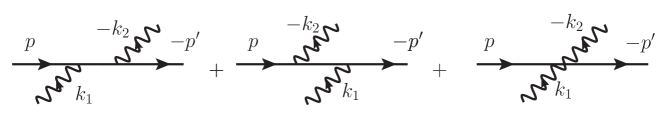
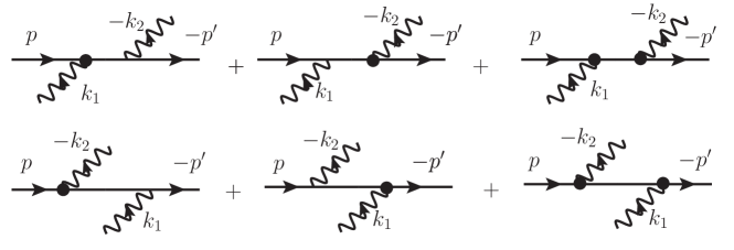
Let us now test our formalism on a recalculation of the Compton scattering amplitude and cross section in spinor QED. We would like to stress once more here that the underlying Feynman rules are not the standard Dirac ones, but second-order rules as explained in part I. As such they contain the diagrams that exist already in scalar QED, depicted in Fig. 1, and other ones involving at least one σμν\sigma^{\mu\nu} (spin) interaction, shown in Fig.2.

Refer to caption
Figure 1: Scalar QED like contributions to the Compton scattering in spinor QED. We use p,k1p,k_{1} as incoming and p,k2-p^{\prime},-k_{2} as outgoing momenta.
Refer to caption
Figure 2: Extra diagrammatic contributions to the spinor case. The bullets represent the coupling with σμν\sigma^{\mu\nu} in the second order formalism, see Fig. 1 of I. We use p,k1p,k_{1} as incoming and p,k2-p^{\prime},-k_{2} as outgoing momenta.

9.1 The N=2 case

For N=2N=2, we already calculated the coefficient functions A2,B2μν,C2A_{2},B_{2{\mu\nu}},C_{2} off-shell in part I using the fermion line master formula, leading to (I 5.19), and we could use these expressions with on-shell conditions, whereafter it is possible to rewrite them in terms of field-strength tensors. Instead, it is more convenient to follow our present approach and get the on-shell coefficient functions using the spin-orbit decomposition from I and the RR-representation.

Using at first the same reference momenta of our scalar calculation above, (67), we find, using (37), (30), and (I 6.9), after simple algebra, the coefficients

A2scal\displaystyle A_{2}^{\rm scal} =\displaystyle= 2r1f1f2r2r1k1r2k2,\displaystyle-2\frac{r_{1}\cdot f_{1}\cdot f_{2}\cdot r_{2}}{r_{1}\cdot k_{1}\,r_{2}\cdot k_{2}}\,,
A2ψ\displaystyle A_{2}^{\psi} =\displaystyle= (12pk1+12pk2)Wη=0=12(12pk1+12pk2)tr(f1f2),\displaystyle-\left(\frac{1}{2p^{\prime}\cdot k_{1}}+\frac{1}{2p^{\prime}\cdot k_{2}}\right)W_{\eta=0}=-\frac{1}{2}\left(\frac{1}{2p^{\prime}\cdot k_{1}}+\frac{1}{2p^{\prime}\cdot k_{2}}\right){\rm tr}\,(f_{1}f_{2})\,,
B2μν\displaystyle B_{2}^{\mu\nu} =\displaystyle= 12r1f1k2f2μν+r2f2k1f1μνr1k1r2k2+12(12pk112pk2)([f1,f2])μν\displaystyle-\frac{1}{2}\frac{r_{1}\cdot f_{1}\cdot k_{2}f_{2}^{\mu\nu}+r_{2}\cdot f_{2}\cdot k_{1}f_{1}^{\mu\nu}}{r_{1}\cdot k_{1}r_{2}\cdot k_{2}}+\frac{1}{2}\left(\frac{1}{2p^{\prime}\cdot k_{1}}-\frac{1}{2p^{\prime}\cdot k_{2}}\right)([f_{1},f_{2}])^{\mu\nu}
C2\displaystyle C_{2} =\displaystyle= 14(12pk1+12pk2)ϵαβγδf1αβf2γδ=12(12pk1+12pk2)tr(f1f~2).\displaystyle-\frac{1}{4}\left(\frac{1}{2p^{\prime}\cdot k_{1}}+\frac{1}{2p^{\prime}\cdot k_{2}}\right)\epsilon_{\alpha\beta\gamma\delta}f_{1}^{\alpha\beta}f_{2}^{\gamma\delta}=\frac{1}{2}\left(\frac{1}{2p^{\prime}\cdot k_{1}}+\frac{1}{2p^{\prime}\cdot k_{2}}\right)\text{tr}(f_{1}\widetilde{f}_{2})\,.

At this stage it becomes clear that the part of each of the reference vectors (67) proportional to their photon’s momentum drops out of the scalar products in each coefficient. As such, we could at this stage replace the rir_{i} by pp^{\prime} without losing information (since this does not invalidate our removal of the more complicated term in R¯2\bar{R}_{2}) – the same is true for scalar QED as is clear from (69) and its correspondence with A2scalA_{2}^{\textrm{scal}}.

Below we shall make use of both representations of the coefficients. In general it is useful to keep the rir_{i} null vectors, for use with the spinor helicity representation (section 3). However, it turns out that for calculating the amplitude in a particular reference frame, it is more convenient to take advantage of the freedom to use ri=pr_{i}=p^{\prime}, since the explicit construction of the spinors |ri|r_{i}\rangle, |ri]|r_{i}] etc, is complicated by their dependence on the photon momenta. On the other hand, at the level of the cross section, spinor products turn into (44-vector) scalar products and here the vector form of the rir_{i} can be applied directly.

9.2 The functions A2,B2αβ,C2A_{2},B_{2{\alpha\beta}},C_{2} with fixed helicities

We begin by providing the coefficients in (LABEL:ABCfinal) in an arbitrary Lorentz frame for the construction of the fully polarised amplitudes in (84) for N=2N=2. Since also the vectors dμd^{\mu} and dμd^{\ast\mu} are defined for an arbitrary frame (likewise zμz^{\mu} and rμr^{\mu} can be chosen with any direction in this frame), this achieves a representation of the polarised amplitudes valid for a general system of reference.

We will denote the polarised amplitudes by 2ssh1h2\mathcal{M}_{2\,s^{\prime}s}^{h_{1}h_{2}}, suppressing the superscript ‘ppp^{\prime}p’ and as above denoting the helicity of photon ii by hih_{i}. For the calculation of 2ss++\mathcal{M}_{2\,s^{\prime}s}^{++}, we require the coefficients

A2scal++\displaystyle A_{2}^{\textrm{scal}++} =2[12]2m2λ1λ2,\displaystyle=-2[12]^{2}\frac{m^{2}}{\lambda_{1}\lambda_{2}}\,,
A2ψ++\displaystyle A_{2}^{\psi++} =12[12]2λ1+λ2λ1λ2,\displaystyle=\frac{1}{2}[12]^{2}\frac{\lambda_{1}+\lambda_{2}}{\lambda_{1}\lambda_{2}}\,,
B2μν++\displaystyle B_{2}^{\mu\nu++} =[12]8λ1λ2[(λ2λ1)[1|[γμ,γν]|2]λ1r12r11[2|[γμ,γν]|2]+λ2r21r22[1|[γμ,γν]|1]]\displaystyle=\frac{[12]}{8\lambda_{1}\lambda_{2}}\Big{[}(\lambda_{2}-\lambda_{1})[1|[\gamma^{\mu},\gamma^{\nu}]|2]-\lambda_{1}\frac{\langle r_{1}2\rangle}{\langle r_{1}1\rangle}[2|[\gamma^{\mu},\gamma^{\nu}]|2]+\lambda_{2}\frac{\langle r_{2}1\rangle}{\langle r_{2}2\rangle}[1|[\gamma^{\mu},\gamma^{\nu}]|1]\Big{]}
=[12]8λ1λ2[(λ2λ1)[1|[γμ,γν]|2][1||2[2|[γμ,γν]|2]+[2||1[1|[γμ,γν]|1]]\displaystyle=\frac{[12]}{8\lambda_{1}\lambda_{2}}\Big{[}(\lambda_{2}-\lambda_{1})[1|[\gamma^{\mu},\gamma^{\nu}]|2]-[1|\not{p}^{\prime}|2\rangle[2|[\gamma^{\mu},\gamma^{\nu}]|2]+[2|\not{p}^{\prime}|1\rangle[1|[\gamma^{\mu},\gamma^{\nu}]|1]\Big{]}
=[12]28λ1λ2[1|[γμ,γν]|1]+2|[γμ,γν]|2]],\displaystyle=\frac{[12]^{2}}{8\lambda_{1}\lambda_{2}}\Big{[}\langle 1|\not{p}^{\prime}[\gamma^{\mu},\gamma^{\nu}]|1]+\langle 2|\not{p}^{\prime}[\gamma^{\mu},\gamma^{\nu}]|2]\Big{]}\,,
C2++\displaystyle C_{2}^{++} =i2[12]2λ1+λ2λ1λ2\displaystyle=-\frac{i}{2}[12]^{2}\frac{\lambda_{1}+\lambda_{2}}{\lambda_{1}\lambda_{2}} (108)

(recall that λi=2pki\lambda_{i}=2p^{\prime}\cdot k_{i}). With these coefficients one readily verifies the general results of sections 6 (equations (82) and (83)) and 8 (equations (99)–(101)). In particular, we shall use the important result C2++=iA2ψ++C_{2}^{++}=-iA_{2}^{\psi++} below. For the amplitudes 2ss+\mathcal{M}_{2\,s^{\prime}s}^{+-} we find

A2scal+\displaystyle A_{2}^{\textrm{scal}+-} =2r12[1r2]r11[2r2]=2[1||22λ1λ2,\displaystyle=-2\frac{\langle r_{1}2\rangle[1r_{2}]}{\langle r_{1}1\rangle[2r_{2}]}=-2\frac{[1|\not{p}^{\prime}|2\rangle^{2}}{\lambda_{1}\lambda_{2}}\,,
A2ψ+\displaystyle A_{2}^{\psi+-} =0,\displaystyle=0\,,
B2μν+\displaystyle B_{2}^{\mu\nu+-} =18λ1λ2[λ1r12[21]r112|[γμ,γν]|2+λ2[r21]12[r22][1|[γμ,γν]|1]]\displaystyle=\frac{1}{8\lambda_{1}\lambda_{2}}\Big{[}\lambda_{1}\frac{\langle r_{1}2\rangle[21]}{\langle r_{1}1\rangle}\langle 2|[\gamma^{\mu},\gamma^{\nu}]|2\rangle+\lambda_{2}\frac{[r_{2}1]\langle 12\rangle}{[r_{2}2]}[1|[\gamma^{\mu},\gamma^{\nu}]|1]\Big{]}
=[1||28λ1λ2[12[1|[γμ,γν]|1][12]2|[γμ,γν]|2],\displaystyle=\frac{[1|\not{p}^{\prime}|2\rangle}{8\lambda_{1}\lambda_{2}}\Big{[}\langle 12\rangle[1|[\gamma^{\mu},\gamma^{\nu}]|1]-[12]\langle 2|[\gamma^{\mu},\gamma^{\nu}]|2\rangle\Big{]}\,,
C2+\displaystyle C_{2}^{+-} =0.\displaystyle=0\,. (109)

Again, these results satisfy the relations given in section 6. These coefficients can be substituted directly into (84) to find the fully polarised amplitudes in any reference frame (we detail the determination of the coefficients αi\alpha_{i} in the following subsection).

9.3 The fully polarised amplitudes

We now further specialise to the centre-of-mass frame, where

pcmμ\displaystyle p_{cm}^{\prime\mu} =Ee(1,βsinθ,0,βcosθ),\displaystyle=-E_{e}\,(1,\beta\sin\theta,0,\beta\cos\theta)\,, pcmμ\displaystyle p_{cm}^{\mu} =Ee(1,0,0,β),\displaystyle=E_{e}\,(1,0,0,\beta)\,,
k1cmμ\displaystyle k_{1\,cm}^{\mu} =Eγ(1,0,0,1),\displaystyle=E_{\gamma}\,(1,0,0,-1)\,, k2cmμ\displaystyle k_{2\,cm}^{\mu} =Eγ(1,sinθ,0,cosθ),\displaystyle=-E_{\gamma}\,(1,-\sin\theta,0,-\cos\theta)\,, (110)

with

β=EγEe,Ee2Eγ2=m2.\displaystyle\beta=\dfrac{E_{\gamma}}{E_{e}},\qquad E^{2}_{e}-E_{\gamma}^{2}=m^{2}. (111)

Measuring the particle spins along their direction of motion (“helicity basis”), we can use the general formulas derived in appendix B with E=E=EeE=E^{\prime}=E_{e} and |𝐩|=|𝐩|=Eγ|{\bf p}|=|{\bf p}^{\prime}|=E_{\gamma}. From (140), (144) and (145) we get

zcmμ\displaystyle z_{cm}^{\mu} =Eem(β,sinθ,0,cosθ),\displaystyle=\dfrac{E_{e}}{m}\,(\beta,\sin\theta,0,\cos\theta)\,, rcmμ\displaystyle r_{cm}^{\mu} =Eem(β,0,0,1),\displaystyle=\dfrac{E_{e}}{m}\,(\beta,0,0,1)\,,
dcmμ\displaystyle d_{cm}^{\mu} =12(0,cosθ,i,sinθ)\displaystyle=\dfrac{1}{2}\,(0,\cos\theta,-i,-\sin\theta) (112)

and the coefficients αi\alpha_{i} can be read off from (146):

α1\displaystyle\alpha_{1} =\displaystyle= 12(1+cosθ)=cos2θ2\displaystyle{1\over 2}(1+\cos\theta)=\cos^{2}\frac{\theta}{2}
α2\displaystyle\alpha_{2} =\displaystyle= Ee2msinθ=Eemsinθ2cosθ2\displaystyle-\frac{E_{e}}{2m}\sin\theta=-\frac{E_{e}}{m}\sin\frac{\theta}{2}\cos\frac{\theta}{2}
α3\displaystyle\alpha_{3} =\displaystyle= Eγ2msinθ=Eγmsinθ2cosθ2\displaystyle-\frac{E_{\gamma}}{2m}\sin\theta=-\frac{E_{\gamma}}{m}\sin\frac{\theta}{2}\cos\frac{\theta}{2}
α4\displaystyle\alpha_{4} =\displaystyle= 0.\displaystyle 0\;. (113)

When written in terms of the Mandelstam variables

s\displaystyle s =\displaystyle= (p+k1)2=(p+k2)2=m2λ2=(Ee+Eγ)2,\displaystyle-(p+k_{1})^{2}=-(p^{\prime}+k_{2})^{2}=m^{2}-\lambda_{2}=(E_{e}+E_{\gamma})^{2}\,,
u\displaystyle u =\displaystyle= (p+k2)2=(p+k1)2=m2λ1=(EeEγ)24Eγ2cos2θ2,\displaystyle-(p+k_{2})^{2}=-(p^{\prime}+k_{1})^{2}=m^{2}-\lambda_{1}=(E_{e}-E_{\gamma})^{2}-4E_{\gamma}^{2}\cos^{2}\dfrac{\theta}{2}\,,
t\displaystyle t =\displaystyle= 2k1k2=2k1k2=4Eγ2sin2θ2.\displaystyle-2k_{1}\cdot k_{2}=-2k_{1}\cdot k_{2}=-4E_{\gamma}^{2}\sin^{2}\dfrac{\theta}{2}\,. (114)

the non-zero coefficients turn into

𝒩α1\displaystyle\mathcal{N}\alpha_{1} =\displaystyle= 2mm4susm2,\displaystyle 2m\dfrac{\sqrt{m^{4}-su}}{s-m^{2}}\,,
𝒩α2\displaystyle\mathcal{N}\alpha_{2} =\displaystyle= s+m2sm2t,\displaystyle-\dfrac{s+m^{2}}{s-m^{2}}\sqrt{-t}\,,
𝒩α3\displaystyle\mathcal{N}\alpha_{3} =\displaystyle= t.\displaystyle-\sqrt{-t}\,. (115)

We shall again provide the amplitudes 2ss++\mathcal{M}_{2\,s^{\prime}s}^{++} and 2ss+\mathcal{M}_{2\,s^{\prime}s}^{+-} using (LABEL:ABCfinal) and (84) in this frame. Since in the coefficients A2,B2μνA_{2},B_{2\mu\nu} and C2C_{2} we represent the field strength tensors in terms of spinor helicity variables, we need the explicit components of the spinors related to the vector k1cmk_{1\,cm} and k2cmk_{2\,cm},

|1a˙\displaystyle|1\rangle^{\dot{a}} =2Eγ(01),\displaystyle=\sqrt{2E_{\gamma}}\begin{pmatrix}0\\ 1\end{pmatrix}, |1]a\displaystyle|1]_{a} =2Eγ(10),\displaystyle=\sqrt{2E_{\gamma}}\begin{pmatrix}-1\\ 0\end{pmatrix}\,,
|2a˙\displaystyle|2\rangle^{\dot{a}} =2Eγ(sinθ2cosθ2),\displaystyle=-\sqrt{2E_{\gamma}}\begin{pmatrix}\sin\frac{\theta}{2}\\ -\cos\frac{\theta}{2}\end{pmatrix}, |2]a\displaystyle|2]_{a} =2Eγ(cosθ2sinθ2).\displaystyle=\sqrt{2E_{\gamma}}\begin{pmatrix}\cos\frac{\theta}{2}\\ \sin\frac{\theta}{2}\end{pmatrix}\,. (116)

For the actual calculation of the coefficients, however, it is now more convenient to replace the ripr_{i}\rightarrow p^{\prime} to avoid having to determine the explicit form of the spinors for the reference vectors in this frame. Doing this in (LABEL:ABCfinal), we obtain,

A2++\displaystyle A_{2}^{++} =t(4m2t)2(sm2)(um2),\displaystyle=\dfrac{t(4m^{2}-t)}{2(s-m^{2})(u-m^{2})}\,,\quad C2++\displaystyle C_{2}^{++} =it22(sm2)(um2),\displaystyle=i\dfrac{t^{2}}{2(s-m^{2})(u-m^{2})}\,, (117)
dB2++p\displaystyle d\cdot B_{2}^{++}\cdot p^{\prime} =m2tt(m4su)4(sm2)2(um2),\displaystyle=m^{2}\,\dfrac{t\sqrt{-t(m^{4}-su)}}{4(s-m^{2})^{2}(u-m^{2})}\,,\quad zB2++p\displaystyle z\cdot B_{2}^{++}\cdot p^{\prime} =mt2(s+m2)4(sm2)2(um2),\displaystyle=-\dfrac{mt^{2}(s+m^{2})}{4(s-m^{2})^{2}(u-m^{2})}\,, (118)

and we can express the remaining scalars in terms of these:

zB2++d\displaystyle z\cdot B_{2}^{++}\cdot d =\displaystyle= 1mdB2++p,\displaystyle\frac{1}{m}d\cdot B_{2}^{++}\cdot p^{\prime}\,, (119)
dB2++d\displaystyle\,d\cdot B_{2}^{++}\cdot d^{\ast} =\displaystyle= 12mzB2++p,\displaystyle\frac{1}{2m}z\cdot B_{2}^{++}\cdot p^{\prime}\,, (120)
zB2++d\displaystyle\;z\cdot B_{2}^{++}\cdot d^{\ast} =\displaystyle= 1mdB2++p,\displaystyle-\frac{1}{m}d\cdot B_{2}^{++}\cdot p^{\prime}\,, (121)
dB2++p\displaystyle d^{\ast}\cdot B_{2}^{++}\cdot p^{\prime} =\displaystyle= dB2++p.\displaystyle d\cdot B_{2}^{++}\cdot p^{\prime}\,. (122)

Using (84), and the above equations, the fully polarised 2ss++\mathcal{M}_{2\,s^{\prime}s}^{++} amplitudes read as,

2++++\displaystyle\mathcal{M}_{2\,++}^{++} =2e2m2tm4su(sm2)2(um2),\displaystyle=-2e^{2}m^{2}\dfrac{t\sqrt{m^{4}-su}}{(s-m^{2})^{2}(u-m^{2})}\,,\quad 2+++\displaystyle\mathcal{M}_{2\,+-}^{++} =2e2m3tt(sm2)2(um2),\displaystyle=-2e^{2}m^{3}\dfrac{t\sqrt{-t}}{(s-m^{2})^{2}(u-m^{2})}\,,
2+++\displaystyle\mathcal{M}_{2\,-+}^{++} =2e2mstt(sm2)2(um2),\displaystyle=2e^{2}m\dfrac{st\sqrt{-t}}{(s-m^{2})^{2}(u-m^{2})}\,,\quad 2++\displaystyle\mathcal{M}_{2\,--}^{++} =2e2m2tm4su(sm2)2(um2).\displaystyle=-2e^{2}m^{2}\dfrac{t\sqrt{m^{4}-su}}{(s-m^{2})^{2}(u-m^{2})}\,. (123)

Likewise for the 2ss+\mathcal{M}_{2\,s^{\prime}s}^{+-} amplitudes we find

A2+\displaystyle A_{2}^{+-} =2(m4su)(sm2)(um2),\displaystyle=\dfrac{-2(m^{4}-su)}{(s-m^{2})(u-m^{2})}\,,\quad C2+\displaystyle C_{2}^{+-} =0,\displaystyle=0\,, (124)
dB2+p\displaystyle d\cdot B_{2}^{+-}\cdot p^{\prime} =(m4su)32t4(sm2)2(um2),\displaystyle=-\dfrac{(m^{4}-su)^{\frac{3}{2}}\sqrt{-t}}{4(s-m^{2})^{2}(u-m^{2})}\,,\quad dB2+p\displaystyle d^{\ast}\cdot B_{2}^{+-}\cdot p^{\prime} =t(m4su)[(sm2)2+m2t]4(sm2)2(um2),\displaystyle=-\dfrac{\sqrt{-t(m^{4}-su)}\left[(s-m^{2})^{2}+m^{2}t\right]}{4(s-m^{2})^{2}(u-m^{2})}, (125)
zB2+p\displaystyle z\cdot B_{2}^{+-}\cdot p^{\prime} =mt(m4su)2(sm2)2(um2),\displaystyle=\dfrac{mt(m^{4}-su)}{2(s-m^{2})^{2}(u-m^{2})}\,,\quad zB2+d\displaystyle z\cdot B_{2}^{+-}\cdot d^{\ast} =t(m4su)[(sm2)2m2t]4m(sm2)2(um2),\displaystyle=-\dfrac{\sqrt{-t(m^{4}-su)}\left[(s-m^{2})^{2}-m^{2}t\right]}{4m(s-m^{2})^{2}(u-m^{2})}, (126)

along with

zB2+d\displaystyle z\cdot B_{2}^{+-}\cdot d =\displaystyle= 1mdB2+p,\displaystyle\frac{1}{m}d\cdot B_{2}^{+-}\cdot p^{\prime}\,, (127)
dB2++d\displaystyle\,d\cdot B_{2}^{++}\cdot d^{\ast} =\displaystyle= 12mzB2+p,\displaystyle\frac{1}{2m}z\cdot B_{2}^{+-}\cdot p^{\prime}\,, (128)

which lead to

2+++\displaystyle\mathcal{M}_{2\,++}^{+-} =2e2(m4su)32(sm2)2(um2),\displaystyle=2e^{2}\dfrac{(m^{4}-su)^{\frac{3}{2}}}{(s-m^{2})^{2}(u-m^{2})}\,,\quad 2++\displaystyle\mathcal{M}_{2\,+-}^{+-} =2e2mt(m4su)(sm2)2(um2),\displaystyle=2e^{2}m\dfrac{\sqrt{-t}(m^{4}-su)}{(s-m^{2})^{2}(u-m^{2})}\,,
2++\displaystyle\mathcal{M}_{2\,-+}^{+-} =2e2mt(m4su)(sm2)2(um2),\displaystyle=-2e^{2}m\dfrac{\sqrt{-t}(m^{4}-su)}{(s-m^{2})^{2}(u-m^{2})}\,,\quad 2+\displaystyle\mathcal{M}_{2\,--}^{+-} =2e2m4su[(sm2)2+m2t](sm2)2(um2).\displaystyle=2e^{2}\dfrac{\sqrt{m^{4}-su}\left[(s-m^{2})^{2}+m^{2}t\right]}{(s-m^{2})^{2}(u-m^{2})}\,. (129)

All these matrix elements agree, up to signs due to differing conventions, with the results presented by Denner and Dittmaier Denner (to be precise, our 2ssh1h2\mathcal{M}_{2\,s^{\prime}s}^{h_{1}h_{2}} corresponds to their 0(s,h1,s,h2)\mathcal{M}_{0}(s,-h_{1},s^{\prime},h_{2}), with a relative sign (1)s+s+h1+h2+1(-1)^{s+s^{\prime}+h_{1}+h_{2}+1}). For historical discussion and derivation of Compton scattering from density matrix and operator techniques, and using the Stokes parameters for the description of polarisation, we refer the reader to fano ; mcmaster .

9.4 Polarised photons, unpolarised electrons

Moving on to the cross section, we can complete the electron spin sums whilst leaving the photon helicities arbitrary. For this calculation, it is useful to use (108) and (109) as they stand (rather than replacing the r1,2r_{1,2} by pp^{\prime}), since upon multiplication of the coefficients with their complex conjugates, the spinor products are turned into 44-vector scalar products. We begin with the amplitudes for the ++++ helicity assignment. Noting that

2k1k2=(λ1+λ2),\displaystyle 2k_{1}\cdot k_{2}=-(\lambda_{1}+\lambda_{2})\,, (130)

we find, after simple algebra,

|A2++|2\displaystyle\left|A_{2}^{++}\right|^{2} =\displaystyle= 1λ12λ22(k1k2)2(λ1+λ2+4p2)2=(λ1+λ2)24λ12λ22(λ1+λ24m2)2,\displaystyle\frac{1}{\lambda_{1}^{2}\lambda_{2}^{2}}\,(k_{1}\cdot k_{2})^{2}(\lambda_{1}+\lambda_{2}+4p^{\prime 2})^{2}=\frac{(\lambda_{1}+\lambda_{2})^{2}}{4\lambda_{1}^{2}\lambda_{2}^{2}}\,(\lambda_{1}+\lambda_{2}-4m^{2})^{2}\,,
B2μν++(B2μν++)\displaystyle B_{2}^{\mu\nu++}(B_{2\mu\nu}^{++})^{\ast} =\displaystyle= 0,\displaystyle 0\,,
|C2++|2\displaystyle\left|C_{2}^{++}\right|^{2} =\displaystyle= 1λ12λ22(k1k2)2(λ1+λ2)2=(λ1+λ2)44λ12λ22,\displaystyle\frac{1}{\lambda_{1}^{2}\lambda_{2}^{2}}\,(k_{1}\cdot k_{2})^{2}(\lambda_{1}+\lambda_{2})^{2}=\frac{(\lambda_{1}+\lambda_{2})^{4}}{4\lambda_{1}^{2}\lambda_{2}^{2}}\,, (131)

so that (91) provides

|2++|2\displaystyle\langle\left|{\cal M}_{2}^{++}\right|^{2}\rangle =\displaystyle= e4(λ1+λ2)24λ12λ22[(λ1+λ24m2)2(λ1+λ2)2].\displaystyle e^{4}\frac{(\lambda_{1}+\lambda_{2})^{2}}{4\lambda_{1}^{2}\lambda_{2}^{2}}\,\Bigl{[}(\lambda_{1}+\lambda_{2}-4m^{2})^{2}-(\lambda_{1}+\lambda_{2})^{2}\Bigr{]}\,. (132)

Note that we could have obtained this result more easily using (65) and (105).

Similarly for the ++- helicity amplitude we find

|A2+|2\displaystyle\left|A_{2}^{+-}\right|^{2} =\displaystyle= 4λ12λ22(2(k1k2)p2λ1λ2)2=4λ12λ22[m2(λ1+λ2)λ1λ2]2,\displaystyle\frac{4}{\lambda_{1}^{2}\lambda_{2}^{2}}\,(2(k_{1}\cdot k_{2})p^{\prime 2}-\lambda_{1}\lambda_{2})^{2}=\frac{4}{\lambda_{1}^{2}\lambda_{2}^{2}}\,\Bigl{[}m^{2}(\lambda_{1}+\lambda_{2})-\lambda_{1}\lambda_{2}\Bigr{]}^{2}\,,
B2μν+(B2μν+)\displaystyle B_{2}^{\mu\nu+-}(B_{2\mu\nu}^{+-})^{\ast} =\displaystyle= 4λ12λ22(k1k2)2(2(k1k2)p2λ1λ2)=(λ1+λ2)2λ12λ22[m2(λ1+λ2)λ1λ2],\displaystyle\frac{4}{\lambda_{1}^{2}\lambda_{2}^{2}}\,(k_{1}\cdot k_{2})^{2}(2(k_{1}\cdot k_{2})p^{\prime 2}-\lambda_{1}\lambda_{2})=\frac{(\lambda_{1}+\lambda_{2})^{2}}{\lambda_{1}^{2}\lambda_{2}^{2}}\Bigl{[}m^{2}(\lambda_{1}+\lambda_{2})-\lambda_{1}\lambda_{2}\Bigr{]}\,,
|C2+|2\displaystyle\left|C_{2}^{+-}\right|^{2} =\displaystyle= 0,\displaystyle 0\,, (133)

giving in total

|2+|2\displaystyle\langle\left|{\cal M}_{2}^{+-}\right|^{2}\rangle =\displaystyle= e42λ12λ22[m2(λ1+λ2)λ1λ2][λ12+λ22+2m2(λ1+λ2)].\displaystyle e^{4}\frac{2}{\lambda_{1}^{2}\lambda_{2}^{2}}\,\Bigl{[}m^{2}(\lambda_{1}+\lambda_{2})-\lambda_{1}\lambda_{2}\Bigr{]}\Bigl{[}\lambda_{1}^{2}+\lambda_{2}^{2}+2m^{2}(\lambda_{1}+\lambda_{2})\Bigr{]}\,. (134)

Writing these results in terms of the usual Mandelstam variables introduced above we arrive at

|2++|2=4e4m2t2(m2t2)(m2u)2(m2s)2,|2+|2=4e4(usm4)(ust22m4)(m2u)2(m2s)2.\displaystyle\begin{split}\langle\left|{\cal M}_{2}^{++}\right|^{2}\rangle&=4e^{4}\frac{m^{2}t^{2}(m^{2}-\frac{t}{2})}{(m^{2}-u)^{2}(m^{2}-s)^{2}}\,,\\ \langle\left|{\cal M}_{2}^{+-}\right|^{2}\rangle&=4e^{4}\frac{(us-m^{4})(us-\frac{t^{2}}{2}-m^{4})}{(m^{2}-u)^{2}(m^{2}-s)^{2}}\,.\end{split} (135)

In the massless limit, this gives the well-known results

|2++|2=0,|2+|2=2e4(su+us).\displaystyle\begin{split}\langle\left|{\cal M}_{2}^{++}\right|^{2}\rangle&=0\,,\\ \langle\left|{\cal M}_{2}^{+-}\right|^{2}\rangle&=-2e^{4}\Bigl{(}\frac{s}{u}+\frac{u}{s}\Bigr{)}\,.\end{split} (136)

Note that, in our conventions, the ++++ amplitude is the helicity violating one, correctly vanishing in the massless case. In the present formalism, it is clear from (131) that this comes about by a cancellation between the AA and CC terms. We discuss some aspects of the massless amplitudes in greater detail in appendix D.

9.5 The unpolarised Compton cross section

Finally, let us also sum over photon polarisations to write down the unpolarised cross section:

12λ,λ|2λλ|2\displaystyle\frac{1}{2}\sum_{\lambda,\lambda^{\prime}}\big{\langle}\big{|}{\cal M}_{2}^{\lambda\lambda^{\prime}}\big{|}^{2}\big{\rangle} =\displaystyle= |2++|2+|2+|2\displaystyle\big{\langle}\left|{\cal M}_{2}^{++}\right|^{2}\big{\rangle}+\big{\langle}\left|{\cal M}_{2}^{+-}\right|^{2}\big{\rangle}
=\displaystyle= 2e4{λ1λ2λ2λ14m2(1λ1+1λ2)+4m4(1λ1+1λ2)2}.\displaystyle 2e^{4}\biggl{\{}-\frac{\lambda_{1}}{\lambda_{2}}-\frac{\lambda_{2}}{\lambda_{1}}-4m^{2}\Bigl{(}\frac{1}{\lambda_{1}}+\frac{1}{\lambda_{2}}\Bigr{)}+4m^{4}\Bigl{(}\frac{1}{\lambda_{1}}+\frac{1}{\lambda_{2}}\Bigr{)}^{2}\biggr{\}}\,.

This is again in agreement, of course, with the standard textbook result, see, for example, eq. (5.87) in peskinschroeder-book .

10 Conclusions and Outlook

In the second part of this series of papers, we have worked out the simplifications that can be achieved using the new, first-quantised worldline representation of the fermion propagator developed in part 1 for the photon-dressed fermion line, when both the fermion legs as well as all photons are taken on-shell (although it should be emphasised that many of the formulas presented here would still be valid if only the fermions were taken on-shell, not the photons). For general kinematics and helicity assignments, we have found three types of simplifications:

  1. 1.

    Most importantly, the “subleading” contributions to the dressed propagator can be omitted.

  2. 2.

    The coefficient functions AN,BNμν,CNA_{N},B_{N{\mu\nu}},C_{N} become manifestly transversal and can be rewritten in terms of photon field-strength tensors in a systematic way.

  3. 3.

    There exist NN-independent relations between those coefficient functions. As a consequence, all on-shell information is contained in the coefficient BNμνB_{N\mu\nu}.

Further simplifications have been exhibited for special kinematics (p=±pp^{\prime}=\pm p) or helicity assignments (the “all +” case). We have also derived recursion formulas for the functions AN,BNμν,CNA_{N},B_{N{\mu\nu}},C_{N} that may become useful as an alternative to the direct calculation methods of I.

On a technical level, we have provided a number of useful relations involving the fixed-helicity photon field-strength tensors, and we have derived explicit formulas for all the relevant Dirac bilinears, for arbitray on-shell momenta p,pp,p^{\prime} and spin vectors r,zr,z. These formulas have allowed us to give expressions for the fully polarised amplitudes valid in an arbitrary Lorentz frame in terms of a canonical set of numerical coefficients and reference vectors defined in that frame. For the fixed-helicity but spin-summed cross sections we have found that the result can be derived purely from the squared moduli of the coefficients.

Applying this machinery to the linear Compton scattering process we have found it to lead to significant simplifications over the standard calculation in the first-order Dirac formalism333R. Stora once told one of the authors (C.S.) that V. Weisskopf was so dissatisfied with the standard textbook calculation of the Compton cross section that he asked not only him, but several others of his PhD students to look for a better way to get the simple final result.. The reasons are easy to pinpoint: first, the encoding of the Dirac algebra structure in the Grassmann path integral replaces the “partially antisymmetric” (in the Lorentz indices) Dirac matrices by the “fully antisymmetric” vectors ημ\eta^{\mu}, and therefore in D=4D=4 leads effectively to an early projection on the Clifford basis, avoiding the appearance of products of more than four Dirac matrices. We find it curious that, although this representation including the “symbol map” have in principle been known for decades fradkin ; fragit , this attractive feature has apparently never been noted. This also implies an early disentanglement of the photon polarisations and fermion spins, allowing them to be treated completely independently. In particular it makes it possible to perform the average over the latter without having to fix the photon number or helicity assignments.

Thus we expect the formalism to be very well-suited for future calculations of non-linear Compton scattering King1 ; Boca1 ; Heinzl1 ; Seipt1 ; Seipt2 ; Boca2 ; King2 , including at higher orders, as well as its crossed process, multiple photon Bremsstrahlung (see, for example, Haug ; Gupta ; Majumdae ; Nadzhafov ; DeCausmaeckerI ; BerendsII ; BerendsIV ; BerendsVI ) and electron-positron annihilation into several photons acfpc ; eidkur ; berkle ; lee-epannihilation . This will, of course, require a computer algebra implementation, which is in progress.

Another very natural application would be to multiloop contributions to the QED anomalous magnetic moment of the type shown in Fig. 3.

Refer to caption
Figure 3: Single fermion line contributions to the QED g2g-2 factor.

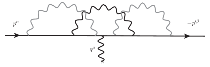
A version of this formalism taylored to this specific purpose (p=pp^{\prime}=-p, one photon taken at low energy, the remaining ones taken off-shell and sewn off in pairs) will be presented elsewhere. As an additional attractive feature, the formalism makes it relatively easy to extract the form factor F2F_{2}.

In the forthcoming third part of this series, we extend the formalism to the construction of the dressed electron propagator in a constant external field, a case where the absence of a practicable extension of the worldline formalism to open fermion lines had been particularly felt (partial results of the third part have already been published in 113 ).

However, there are many other possible generalisations, let us mention here only a few:

As a final remark, let us emphasise that although here we have focused on the implementation of the formalism in terms of path integrals, nowadays often simply called the “worldline formalism,” we could also have worked more directly with the Feynman diagrams of the second-order formalism. However, such an approach would obscure some of the important advantages of the formalism, such as its ability to combine Feynman diagrams that differ only by the position of the photon legs along the fermion line, and the flexibility provided by IBP in the proper-time parameters.

Acknowledgements.
We thank P. Cvitanović, G.V. Dunne and A. Ilderton for useful conversations and correspondence. CS and JPE thank CONACYT for support through project Ciencias Basicas 2014 No. 242461. JPE further acknowledges financial support from UMSNH through CiC project #483224-2019. VMBG received support from PRODEP project 511-6/19-4990 for part of this work.

Appendix A Conventions

On the side of the worldline formalism, we work in Euclidean space with metric (++++)(+++\,+), and use Dirac matrices fulfilling {γμ,γν}=2δμν\{\gamma^{\mu},\gamma^{\nu}\}=-2\delta^{\mu\nu}. On the field theory side, we Wick rotate to Minkowski space with metric ημν=diag(+++)\eta_{\mu\nu}=\textrm{diag}(-++\,+), and use {γμ,γν}=2ημν\{\gamma^{\mu},\gamma^{\nu}\}=-2\eta^{\mu\nu}. We further define ε0123=+1\varepsilon^{0123}=+1 and γ5=iγ0γ1γ2γ3\gamma_{5}=i\gamma^{0}\gamma^{1}\gamma^{2}\gamma^{3}. These Minkowski space conventions coincide with the textbook of Srednicki srednicki-book except for the sign of the electric charge, and the fact that we use all ingoing momenta in Feynman diagrams instead of all outgoing ones.

Appendix B Special cases of Dirac bilinears

In this appendix, which supplements section 5, we compute the coefficients α1,,α4\alpha_{1},\ldots,\alpha_{4} explicitly for the electron-electron case and for the two most common choices of the spin-axis vectors rμr^{\mu} and zμz^{\mu}, corresponding to a projection on the electron’s direction of motion (the helicity basis) or on the direction corresponding to the zz-axis in its rest frame. As an overall convention, we take the ingoing electron to move along the zz axis and the outgoing one in the xx-zz plane. Thus we can write their four-vectors as

pμ=(E,0,0,|𝐩|),pμ=(E,|𝐩|sinθ,0,|𝐩|cosθ).\displaystyle p^{\mu}=(E,0,0,|{\bf p}|)\,,\quad-{p^{\prime}}^{\mu}=(E^{\prime},|{\bf p}^{\prime}|\sin\theta,0,|{\bf p}^{\prime}|\cos\theta)\;. (138)

B.1 Standard basis

If we use the most common definition of the electron polarizations, the vectors rμr^{\mu} and zμz^{\mu} are taken as (0,0,0,1)(0,0,0,1) in the respective rest frames, and then subjected to the same Lorentz boost that brings their electron up to speed. With our convention (138) this results in

rμ\displaystyle r^{\mu} =1m(|𝐩|,0,0,E)\displaystyle=\frac{1}{m}(|{\bf p}|,0,0,E) (139)
zμ\displaystyle z^{\mu} =1m(|𝐩|cosθ,(Em)cosθsinθ,0,Ecos2θ+msin2θ).\displaystyle=\frac{1}{m}\bigl{(}|{\bf p}^{\prime}|\cos\theta,(E^{\prime}-m)\cos\theta\sin\theta,0,E^{\prime}\cos^{2}\theta+m\sin^{2}\theta\bigr{)}. (140)

Finally, the null vector (72)

dμ\displaystyle d^{\mu} =14mu¯+(p)γμγ5u(p)\displaystyle=\dfrac{1}{4m}\overline{u}_{+}(-p^{\prime})\gamma^{\mu}\gamma_{5}u_{-}(-p^{\prime}) (141)

must be constructed using the corresponding spinorial Lorentz boost. This gives, after a lengthy but simple calculation,

dμ=12m(|𝐩|sinθ,Esin2θ+mcos2θ,im,(Em)sinθcosθ).\displaystyle d^{\mu}=\frac{1}{2m}\bigl{(}|{\bf p}^{\prime}|\sin\theta,E^{\prime}\sin^{2}\theta+m\cos^{2}\theta,-im,(E^{\prime}-m)\sin\theta\cos\theta\bigr{)}\;. (142)

This is all we need for the evaluation of (73). One finds, after substantial cancellations,

4m2α1\displaystyle 4m^{2}\alpha_{1} =\displaystyle= (E+m)(E+m)2|𝐩||𝐩|cosθ+(Em)(Em)cos2θ\displaystyle(E+m)(E^{\prime}+m)-2|{\bf p}||{\bf p}^{\prime}|\cos\theta+(E-m)(E^{\prime}-m)\cos^{2}\theta
4m2α2\displaystyle 4m^{2}\alpha_{2} =\displaystyle= |𝐩||𝐩|sinθ+(Em)(Em)sinθcosθ\displaystyle-|{\bf p}||{\bf p}^{\prime}|\sin\theta+(E-m)(E^{\prime}-m)\sin\theta\cos\theta
4m2α3\displaystyle 4m^{2}\alpha_{3} =\displaystyle= |𝐩|(Em)sinθcosθ|𝐩|(E+m)sinθ\displaystyle|{\bf p}|(E^{\prime}-m)\sin\theta\cos\theta-|{\bf p}^{\prime}|(E+m)\sin\theta
4m2α4\displaystyle 4m^{2}\alpha_{4} =\displaystyle= |𝐩|[(E+m)+(Em)cos2θ]+2E|𝐩|cosθ.\displaystyle-|{\bf p}|\bigl{[}(E^{\prime}+m)+(E^{\prime}-m)\cos^{2}\theta\bigr{]}+2E|{\bf p}^{\prime}|\cos\theta\;. (143)

B.2 Helicity basis

Due to our convention of the incoming particle moving in the zz direction, changing to the helicity basis leaves rμr^{\mu} unchanged. The vectors zμz^{\mu} and dμd^{\mu} become simpler:

zμ\displaystyle z^{\mu} =\displaystyle= 1m(|𝐩|,Esinθ,0,Ecosθ)\displaystyle\frac{1}{m}(|{\bf p}^{\prime}|,E^{\prime}\sin\theta,0,E^{\prime}\cos\theta) (144)
dμ\displaystyle d^{\mu} =\displaystyle= 12(0,cosθ,i,sinθ).\displaystyle\frac{1}{2}(0,\cos\theta,-i,-\sin\theta)\;. (145)

The coefficients also simplify,

4m2α1\displaystyle 4m^{2}\alpha_{1} =\displaystyle= (EE|𝐩||𝐩|+m2)(1+cosθ)\displaystyle(EE^{\prime}-|{\bf p}||{\bf p}^{\prime}|+m^{2})(1+\cos\theta)
4m2α2\displaystyle 4m^{2}\alpha_{2} =\displaystyle= m(E+E)sinθ\displaystyle-m(E+E^{\prime})\sin\theta
4m2α3\displaystyle 4m^{2}\alpha_{3} =\displaystyle= m(|𝐩|+|𝐩|)sinθ\displaystyle-m(|{\bf p}|+|{\bf p}^{\prime}|)\sin\theta
4m2α4\displaystyle 4m^{2}\alpha_{4} =\displaystyle= (E|𝐩|E|𝐩|)(1+cosθ).\displaystyle(E|{\bf p}^{\prime}|-E^{\prime}|{\bf p}|)(1+\cos\theta)\;. (146)

Note that in the case of forward scattering, θ=0\theta=0, both bases coincide. If the scattering is forward and elastic, |𝐩|=|𝐩||{\bf p}|=|{\bf p}^{\prime}|, the coefficients become trivial, α1=1,α2=α3=α4=0\alpha_{1}=1,\alpha_{2}=\alpha_{3}=\alpha_{4}=0.

Appendix C Recursion relations for kernel coefficients

Various relations between the coefficients, ANA_{N}, BNμνB_{N\mu\nu} and CNC_{N} have been presented in the main text. Here we follow a different path, taking advantage of the definition of the kernel as the inverse of a Klein-Gordon-like operator, to derive some recursive identities that hold between coefficients for different numbers of photons. These could be useful if one had already determined the coefficients up to a given NN, since they can be used to produce the coefficients at order N+1N+1 and higher.

Scalar QED

Beginning with scalar QED the full scalar propagator, DxxD^{x^{\prime}x}, is the inverse of the Klein-Gordon operator in position space so that it satisfies the defining equation:

(D2+m2)Dxx=x|x=δD(xx).(-D^{\prime 2}+m^{2})D^{x^{\prime}x}=\langle x^{\prime}|x\rangle=\delta^{D}(x^{\prime}-x)\,. (147)

Our path integral representation of the NN-photon dressed propagator, (I.2.1) and (LABEL:linemastercov) is an inverse for this operator projected onto the subspace multi-linear in photon polarisations. Thus, writing the propagator as a sum over photon numbers,

D=D0+D1+,D=D_{0}+D_{1}+\ldots\,, (148)

where the term DND_{N} is taken multi-linear in ε1εN\varepsilon_{1}\ldots\varepsilon_{N}, the defining equation (147) in momentum space becomes

(p2+m2)Dppeiεi(2p+ki)Dp+ki,p+e2i,jεiεjDp+ki+kj,p|multi=(2π)DδD(p+p),(p^{\prime 2}+m^{2})D^{p\prime p}-e\sum_{i}\varepsilon_{i}\cdot(2p^{\prime}+k_{i})D^{p^{\prime}+k_{i},p}+e^{2}\sum_{i,j}\varepsilon_{i}\cdot\varepsilon_{j}D^{p^{\prime}+k_{i}+k_{j},p}\Big{|}_{\textrm{multi}}=(2\pi)^{D}\delta^{D}(p^{\prime}+p)\,, (149)

where we truncate at some multi-linear order. Defining the amputated propagator via

DN:=D^N(p2+m2)(p2+m2)D_{N}:=\frac{\widehat{D}_{N}}{(p^{\prime 2}+m^{2})(p^{2}+m^{2})} (150)

we extract the 𝒪(ε1εN)\mathcal{O}(\varepsilon_{1}\ldots\varepsilon_{N}) contribution to find a recursion relation,

D^Npp\displaystyle\widehat{D}^{p^{\prime}p}_{N} =(p2+m2)[ei=1Nεi(2p+ki)DN1p+ki,p(ε1,k1;;εi^,k^i;;εN,kN)\displaystyle=(p^{2}+m^{2})\Big{[}e\sum_{i=1}^{N}\varepsilon_{i}\cdot(2p^{\prime}+k_{i})D_{N-1}^{p^{\prime}+k_{i},p}(\varepsilon_{1},k_{1};\ldots;\hat{\varepsilon_{i}},\hat{k}_{i};\ldots;\varepsilon_{N},k_{N})
e2ijNεiεjDN2p+ki+kj,p(ε1,k1;;εi^,k^i;;εj^,k^i;;εN,kN)],\displaystyle-e^{2}\sum_{i\neq j}^{N}\varepsilon_{i}\cdot\varepsilon_{j}D_{N-2}^{p^{\prime}+k_{i}+k_{j},p}(\varepsilon_{1},k_{1};\ldots;\hat{\varepsilon_{i}},\hat{k}_{i};\ldots;\hat{\varepsilon_{j}},\hat{k}_{i};\ldots;\varepsilon_{N},k_{N})\Big{]}\,, (151)

where as usual the hat indicates that the variable is removed. The terms in brackets represent the addition of extra (scalar QED) vertices glued on to a sum of (N1)(N-1)- and (N2)(N-2)-photon amplitudes to “promote” them to an NN-photon amplitude.

In the case of on-shell photons, we can simplify the recursion relation by replacing the polarisation vectors εiμ\varepsilon_{i\,\mu} according to

εipfipki,\varepsilon_{i}\longrightarrow\dfrac{p^{\prime}\cdot f_{i}}{p^{\prime}\cdot k_{i}}, (152)

in the recursion relation, which then turns into

D^Npp\displaystyle\widehat{D}^{p^{\prime}p}_{N} =e2(p2+m2)ijNpfifjppkipkjDN2p+ki+kj,p(ε1,k1;;εi^,k^i;;εj^,k^i;;εN,kN).\displaystyle=e^{2}(p^{2}+m^{2})\,\sum_{i\neq j}^{N}\dfrac{p^{\prime}\cdot f_{i}\cdot f_{j}\cdot p^{\prime}}{p^{\prime}\cdot k_{i}p^{\prime}\cdot k_{j}}\,D_{N-2}^{p^{\prime}+k_{i}+k_{j},p}(\varepsilon_{1},k_{1};\ldots;\hat{\varepsilon_{i}},\hat{k}_{i};\ldots;\hat{\varepsilon_{j}},\hat{k}_{i};\ldots;\varepsilon_{N},k_{N}). (153)

So if we use the RR-representation of the amplitude, (29), then we produce the NN-photon propagator already written in a manifestly gauge invariant way.

Spinor QED

For the spinor case we proceed analogously, but with respect to the kernel KK, (2) which is a Green function for the Klein-Gordon plus spin coupling operator,

(D2+m2+ie2σμνFμν)Kxx=δD(xx).(-D^{\prime 2}+m^{2}+\frac{ie}{2}\sigma^{\mu\nu}F_{\mu\nu})K^{x^{\prime}x}=\delta^{D}(x^{\prime}-x)\,. (154)

Going to momentum space and projecting onto terms multi-linear in photon polarisation leads to the requirement that

(p2+m2)Kpp\displaystyle(p^{\prime 2}+m^{2})K^{p\prime p} eiεi(2p+ki)Kp+ki,pe2iσμνfiμνKp+ki,p\displaystyle-e\sum_{i}\varepsilon_{i}\cdot(2p^{\prime}+k_{i})K^{p^{\prime}+k_{i},p}-\frac{e}{2}\sum_{i}\sigma^{\mu\nu}f_{i\,\mu\nu}K^{p^{\prime}+k_{i},p}
+e2i,jεiεjKp+ki+kj,p|multi=(2π)DδD(p+p).\displaystyle+e^{2}\sum_{i,j}\varepsilon_{i}\cdot\varepsilon_{j}K^{p^{\prime}+k_{i}+k_{j},p}\Big{|}_{\textrm{multi}}=(2\pi)^{D}\delta^{D}(p^{\prime}+p)\,. (155)

If we now also use the identification (11)

KNpp(ie)N𝔎Npp(p2+m2)(p2+m2),K_{N}^{p^{\prime}p}\equiv(-ie)^{N}\frac{\mathfrak{K}_{N}^{p^{\prime}p}}{(p^{\prime 2}+m^{2})(p^{2}+m^{2})}\,, (156)

then we can solve the relation for the 𝔎N\mathfrak{K}_{N}, for N1N\geqslant 1:

𝔎Npp\displaystyle\mathfrak{K}_{N}^{p^{\prime}p} =iiεi(2p+ki)(p+ki)2+m2𝔎N1p+ki,p+i2iσμνfiμν(p+ki)2+m2𝔎N1p+ki,p\displaystyle=i\sum_{i}\frac{\varepsilon_{i}\cdot(2p^{\prime}+k_{i})}{(p^{\prime}+k_{i})^{2}+m^{2}}\mathfrak{K}_{N-1}^{p^{\prime}+k_{i},p}+\frac{i}{2}\sum_{i}\frac{\sigma^{\mu\nu}f_{i\,\mu\nu}}{(p^{\prime}+k_{i})^{2}+m^{2}}\mathfrak{K}_{N-1}^{p^{\prime}+k_{i},p}
+ijεiεj(p+ki+kj)2+m2𝔎N2p+ki+kj,p.\displaystyle+\sum_{i\neq j}\frac{\varepsilon_{i}\cdot\varepsilon_{j}}{(p^{\prime}+k_{i}+k_{j})^{2}+m^{2}}\mathfrak{K}_{N-2}^{p^{\prime}+k_{i}+k_{j},p}\,. (157)

This equation is analogous to (151), but with the inclusion of the additional spin vertex present in the second order Feynman rules. Now we decompose the matrix structure as in (14) and find three recursion relations between the coefficients. Firstly for AA,

ANpp\displaystyle A_{N}^{p^{\prime}p} =ii[εi(2p+ki)(p+ki)2+m2AN1p+ki,p(ε^i,k^i)+fiμν(p+ki)2+m2BN1,νμp+ki,p(ε^i,k^i)]\displaystyle=i\sum_{i}\Big{[}\frac{\varepsilon_{i}\cdot(2p^{\prime}+k_{i})}{(p^{\prime}+k_{i})^{2}+m^{2}}A_{N-1}^{p^{\prime}+k_{i},p}(\hat{\varepsilon}_{i},\hat{k}_{i})+\frac{f_{i\,\mu\nu}}{(p^{\prime}+k_{i})^{2}+m^{2}}B_{N-1,\nu\mu}^{p^{\prime}+k_{i},p}(\hat{\varepsilon}_{i},\hat{k}_{i})\Big{]}
+ijεiεj(p+ki+kj)2+m2AN2p+ki+kj,p(ε^i,k^i,ε^j,k^j),\displaystyle+\sum_{i\neq j}\frac{\varepsilon_{i}\cdot\varepsilon_{j}}{(p^{\prime}+k_{i}+k_{j})^{2}+m^{2}}A_{N-2}^{p^{\prime}+k_{i}+k_{j},p}(\hat{\varepsilon}_{i},\hat{k}_{i},\hat{\varepsilon}_{j},\hat{k}_{j})\,, (158)

then for BB:

BNαβpp\displaystyle B_{N\alpha\beta}^{p^{\prime}p} =ii[εi(2p+ki)(p+ki)2+m2BN1,αβp+ki,p(ε^i,k^i)2fiμβ(p+ki)2+m2BN1p+ki,p,μ(ε^i,k^i)α]\displaystyle=i\sum_{i}\Big{[}\frac{\varepsilon_{i}\cdot(2p^{\prime}+k_{i})}{(p^{\prime}+k_{i})^{2}+m^{2}}B_{N-1,\alpha\beta}^{p^{\prime}+k_{i},p}(\hat{\varepsilon}_{i},\hat{k}_{i})-2\frac{f_{i\,\mu\beta}}{(p^{\prime}+k_{i})^{2}+m^{2}}B_{N-1}^{p^{\prime}+k_{i},p,\mu}{}_{\alpha}(\hat{\varepsilon}_{i},\hat{k}_{i})\Big{]}
+i2i[fiαβ(p+ki)2+m2AN1p+ki,p(ε^i,k^i)+f~iαβ(p+ki)2+m2CN1p+ki,p(ε^i,k^i)]\displaystyle+\frac{i}{2}\sum_{i}\Big{[}\frac{f_{i\,\alpha\beta}}{(p^{\prime}+k_{i})^{2}+m^{2}}A_{N-1}^{p^{\prime}+k_{i},p}(\hat{\varepsilon}_{i},\hat{k}_{i})+\frac{{\widetilde{f}}_{i}^{\alpha\beta}}{(p^{\prime}+k_{i})^{2}+m^{2}}C_{N-1}^{p^{\prime}+k_{i},p}(\hat{\varepsilon}_{i},\hat{k}_{i})\Big{]}
+ijεiεj(p+ki+kj)2+m2BN2,αβp+ki+kj,p(ε^i,k^i,ε^j,k^j),\displaystyle+\sum_{i\neq j}\frac{\varepsilon_{i}\cdot\varepsilon_{j}}{(p^{\prime}+k_{i}+k_{j})^{2}+m^{2}}B_{N-2,\alpha\beta}^{p^{\prime}+k_{i}+k_{j},p}(\hat{\varepsilon}_{i},\hat{k}_{i},\hat{\varepsilon}_{j},\hat{k}_{j})\,, (159)

and finally for CC,

CNpp\displaystyle C_{N}^{p^{\prime}p} =i2i[2εi(2p+ki)(p+ki)2+m2CN1p+ki,p(ε^i,k^i)+ϵμνρσfiμν(p+ki)2+m2BN1,ρσp+ki,p(ε^i,k^i)]\displaystyle=\frac{i}{2}\sum_{i}\Big{[}2\frac{\varepsilon_{i}\cdot(2p^{\prime}+k_{i})}{(p^{\prime}+k_{i})^{2}+m^{2}}C_{N-1}^{p^{\prime}+k_{i},p}(\hat{\varepsilon}_{i},\hat{k}_{i})+\frac{\epsilon^{\mu\nu\rho\sigma}f_{i\,\mu\nu}}{(p^{\prime}+k_{i})^{2}+m^{2}}B_{N-1,\rho\sigma}^{p^{\prime}+k_{i},p}(\hat{\varepsilon}_{i},\hat{k}_{i})\Big{]}
+ijεiεj(p+ki+kj)2+m2CN2p+ki+kj,p(ε^i,k^i,ε^j,k^j).\displaystyle+\sum_{i\neq j}\frac{\varepsilon_{i}\cdot\varepsilon_{j}}{(p^{\prime}+k_{i}+k_{j})^{2}+m^{2}}C_{N-2}^{p^{\prime}+k_{i}+k_{j},p}(\hat{\varepsilon}_{i},\hat{k}_{i},\hat{\varepsilon}_{j},\hat{k}_{j})\,. (160)

These can be used to convert the N=2N=2 coefficients presented in the main text into the coefficients for N=3N=3 and greater numbers of photons.

There are two simplification that can be made on-shell. Firstly, the relations between coefficients, (80) and (82), allow for the right hand sides of the recursion relations to be written entirely in terms of the BB and B~\widetilde{B}. Secondly, since AN,BNαβ,CNA_{N},B_{N\,\alpha\beta},C_{N} are transversal on-shell, we can again substitute εipfipki\varepsilon_{i}\rightarrow\dfrac{p^{\prime}\cdot f_{i}}{p^{\prime}\cdot k_{i}}, to rewrite the relations in terms of the field strength tensors of the photons. Since all on-shell information is contained in BNαβB_{N\,\alpha\beta}, it suffices to give this coefficient. For N=2N=2, we have

B2αβpp\displaystyle B_{2\alpha\beta}^{p^{\prime}p} =ii(p+ki)2+m2[2fiμβB1p+ki,p,μ(ε^i,k^i)α+12A1p+ki,p(ε^i,k^i)fiαβ],\displaystyle=\sum_{i}\dfrac{i}{(p^{\prime}+k_{i})^{2}+m^{2}}\Big{[}-2f_{i\,\mu\beta}B_{1}^{p^{\prime}+k_{i},p,\mu}{}_{\alpha}(\hat{\varepsilon}_{i},\hat{k}_{i})+\dfrac{1}{2}A_{1}^{p^{\prime}+k_{i},p}(\hat{\varepsilon}_{i},\hat{k}_{i})f_{i\,\alpha\beta}\Big{]}, (161)

with

B1αβpp\displaystyle B^{p^{\prime}p}_{1\,\alpha\beta} =\displaystyle= i2fαβ,A1pp=irf(pp)rk.\displaystyle\dfrac{i}{2}f_{\alpha\beta},\qquad\qquad A^{p^{\prime}p}_{1}=-\dfrac{ir\cdot f\cdot(p-p^{\prime})}{r\cdot k}. (162)

In the general case, (N>2N>2)

BNαβpp\displaystyle B_{N\alpha\beta}^{p^{\prime}p} =ii1(p+ki)2+m2[pBN1p+ki,p(ε^i,k^i)(p+ki)m2p(p+ki)fiαβ+pB~N1p+ki,p(ε^i,k^i)(p+ki)m2+p(p+ki)f~iαβ\displaystyle=i\sum_{i}\dfrac{1}{(p^{\prime}+k_{i})^{2}+m^{2}}\Big{[}\dfrac{p\cdot B_{N-1}^{p^{\prime}+k_{i},p}(\hat{\varepsilon}_{i},\hat{k}_{i})\cdot(p^{\prime}+k_{i})}{m^{2}-p\cdot(p^{\prime}+k_{i})}f_{i\,\alpha\beta}+\dfrac{p\cdot\widetilde{B}_{N-1}^{p^{\prime}+k_{i},p}(\hat{\varepsilon}_{i},\hat{k}_{i})\cdot(p^{\prime}+k_{i})}{m^{2}+p\cdot(p^{\prime}+k_{i})}{\widetilde{f}}_{i\alpha\beta}
2fiμβBN1p+ki,p,μ(ε^i,k^i)α]ij(1(p+ki+kj)2+m2)(pfifjppkipkj)BN2,αβp+ki+kj,p(ε^i,k^i,ε^j,k^j).\displaystyle-2f_{i\,\mu\beta}B_{N-1}^{p^{\prime}+k_{i},p,\mu}{}_{\alpha}(\hat{\varepsilon}_{i},\hat{k}_{i})\Big{]}-\sum_{i\neq j}\left(\frac{1}{(p^{\prime}+k_{i}+k_{j})^{2}+m^{2}}\right)\left(\dfrac{p^{\prime}\cdot f_{i}\cdot f_{j}\cdot p^{\prime}}{p^{\prime}\cdot k_{i}p^{\prime}\cdot k_{j}}\right)B_{N-2,\alpha\beta}^{p^{\prime}+k_{i}+k_{j},p}(\hat{\varepsilon}_{i},\hat{k}_{i},\hat{\varepsilon}_{j},\hat{k}_{j})\,. (163)

Now we have a manifestly gauge invariant recursion relation that can be used to determine the coefficients at order NN from those of lower order.

Appendix D Helicity amplitudes in the massless limit

In the worldline formalism the massless fermion amplitudes corresponding to (9) can be obtained in two ways. One of them is using the formula (13) and computing the limit when m0m\rightarrow 0,

Nsspp=limm0(ie)N2mu¯s(p)𝔎Nppus(p).\displaystyle{\cal M}_{Ns^{\prime}s}^{p^{\prime}p}=\lim_{m\rightarrow 0}\frac{(-ie)^{N}}{2m}\bar{u}_{s^{\prime}}(-p^{\prime})\mathfrak{K}_{N}^{p^{\prime}p}u_{s}(p). (164)

The second way is by setting first m=0m=0 in (9), and then taking the limit when p20p^{2}\rightarrow 0. With the aid of equations (8) and (11), we arrive at

Nsspp\displaystyle{\cal M}_{Ns^{\prime}s}^{p^{\prime}p} =\displaystyle= (ie)N(limp20[u¯s(p)𝔎Nppp2us(p)]|p2=p2+ii=1Nu¯s(p)ε̸i𝔎N1p+ki,p(p+ki)2us(p)),\displaystyle(-ie)^{N}\left(\lim_{p^{2}\rightarrow 0}\left.\left[\bar{u}_{s^{\prime}}(-p^{\prime})\frac{\mathfrak{K}_{N}^{p^{\prime}p}}{\sqrt{-p^{2}}}u_{s}(p)\right]\right|_{p^{\prime 2}=p^{2}}+i\sum_{i=1}^{N}\,\bar{u}_{s^{\prime}}(-p^{\prime})\,\not{\varepsilon}_{i}\frac{\mathfrak{K}_{N-1}^{p^{\prime}+k_{i},p}}{(p^{\prime}+k_{i})^{2}}u_{s}(p)\right),

where the spinors in the subleading contribution satisfy the massless on-shell relations in (10).

The leading contribution in (LABEL:am_massless_prev) is equivalent to

limm0(ie)Nmu¯s(p)𝔎Nppus(p).\displaystyle\lim_{m\rightarrow 0}\frac{(-ie)^{N}}{m}\bar{u}_{s^{\prime}}(-p^{\prime})\mathfrak{K}_{N}^{p^{\prime}p}u_{s}(p). (166)

Then, from (164) and (LABEL:am_massless_prev), we obtain the second formula to compute the massless amplitude,

Nsspp\displaystyle{\cal M}_{Ns^{\prime}s}^{p^{\prime}p} =\displaystyle= e(ie)N1i=1Nu¯s(p)ε̸i𝔎N1p+ki,p(p+ki)2us(p)\displaystyle-e(-ie)^{N-1}\sum_{i=1}^{N}\,\bar{u}_{s^{\prime}}(-p^{\prime})\,\not{\varepsilon}_{i}\frac{\mathfrak{K}_{N-1}^{p^{\prime}+k_{i},p}}{(p^{\prime}+k_{i})^{2}}u_{s}(p) (167)

that now comes only from the subleading piece that depends upon the kernel with N1N-1 photons. Let us corroborate that both (164) and (167) give the correct amplitude for N=1,2N=1,2. According to (I 5.13), (I 5.14), and (I 5.20), we obtain that,

𝔎0pp\displaystyle\mathfrak{K}_{0}^{p^{\prime}p} =\displaystyle= p2+m2=p2+m2,\displaystyle p^{2}+m^{2}=p^{\prime 2}+m^{2}\,, (168)
𝔎1pp\displaystyle\mathfrak{K}_{1}^{p^{\prime}p} =\displaystyle= i(ε̸ε̸),\displaystyle i\left(\not{\varepsilon}{\not{p}}-{\not{p}}^{\prime}\not{\varepsilon}\right)\,, (169)
𝔎2pp\displaystyle\mathfrak{K}_{2}^{p^{\prime}p} =\displaystyle= 1m2+(p+k1)2[ε̸1(+1+m)ε̸2(m)(m)ε̸1ε̸2(m)\displaystyle\frac{-1}{m^{2}+(p^{\prime}+k_{1})^{2}}\Bigl{[}-\not{\varepsilon}_{1}(\not{p}^{\prime}+\not{k}_{1}+m)\not{\varepsilon}_{2}(\not{p}-m)-(\not{p}^{\prime}-m)\not{\varepsilon}_{1}\not{\varepsilon}_{2}(\not{p}-m) (170)
+(m)ε̸1(+1m)ε̸2]+(12).\displaystyle\hskip 100.0pt+(\not{p}^{\prime}-m)\not{\varepsilon}_{1}(\not{p}^{\prime}+\not{k}_{1}-m)\not{\varepsilon}_{2}\Bigr{]}+(1\leftrightarrow 2).

Using the formula (164), the amplitude for N=1N=1 is calculated as,

1sspp\displaystyle{\cal M}_{1s^{\prime}s}^{p^{\prime}p} =\displaystyle= limm0e2mu¯s(p)(ε̸ε̸)us(p)\displaystyle\lim_{m\rightarrow 0}\frac{e}{2m}\bar{u}_{s^{\prime}}(-p^{\prime})\left(\not{\varepsilon}{\not{p}}-{\not{p}}^{\prime}\not{\varepsilon}\right)u_{s}(p) (171)
=\displaystyle= limm0(2me2mu¯s(p)ε̸us(p))\displaystyle\lim_{m\rightarrow 0}\Bigl{(}-2m\,\frac{e}{2m}\bar{u}_{s^{\prime}}(-p^{\prime})\not{\varepsilon}u_{s}(p)\Bigr{)}
=\displaystyle= u¯s(p)ε̸us(p),\displaystyle-\bar{u}_{s^{\prime}}(-p^{\prime})\not{\varepsilon}u_{s}(p)\,,

where before the limiting process we have used the on-shell relations (10). The result in (171) is the same as the one computed from the standard formalism using Feynman diagrams. Similarly for N=2N=2, we obtain that

2sspp\displaystyle{\cal M}_{2s^{\prime}s}^{p^{\prime}p} =\displaystyle= limm0e22mu¯s(p)(1m2+(p+k1)2[ε̸1(+1+m)ε̸2(m)(m)ε̸1ε̸2(m)\displaystyle\lim_{m\rightarrow 0}\frac{e^{2}}{2m}\bar{u}_{s^{\prime}}(-p^{\prime})\Big{(}\frac{1}{m^{2}+(p^{\prime}+k_{1})^{2}}\Bigl{[}-\not{\varepsilon}_{1}(\not{p}^{\prime}+\not{k}_{1}+m)\not{\varepsilon}_{2}(\not{p}-m)-(\not{p}^{\prime}-m)\not{\varepsilon}_{1}\not{\varepsilon}_{2}(\not{p}-m) (172)
+(m)ε̸1(+1m)ε̸2]+(12))us(p)\displaystyle\hskip 100.0pt+(\not{p}^{\prime}-m)\not{\varepsilon}_{1}(\not{p}^{\prime}+\not{k}_{1}-m)\not{\varepsilon}_{2}\Bigr{]}+(1\leftrightarrow 2)\Big{)}u_{s}(p)
=\displaystyle= limm02me22mu¯s(p)(ε̸1(+1+m)ε̸2m2+(p+k1)2+(12))us(p)\displaystyle\lim_{m\rightarrow 0}2m\frac{e^{2}}{2m}\bar{u}_{s^{\prime}}(-p^{\prime})\left(\frac{\not{\varepsilon}_{1}(\not{p}^{\prime}+\not{k}_{1}+m)\not{\varepsilon}_{2}}{m^{2}+(p^{\prime}+k_{1})^{2}}+(1\leftrightarrow 2)\right)u_{s}(p)
=\displaystyle= e2u¯s(p)(ε̸1(+1)ε̸2(p+k1)2+(12))us(p),\displaystyle e^{2}\bar{u}_{s^{\prime}}(-p^{\prime})\left(\frac{\not{\varepsilon}_{1}(\not{p}^{\prime}+\not{k}_{1})\not{\varepsilon}_{2}}{(p^{\prime}+k_{1})^{2}}+(1\leftrightarrow 2)\right)u_{s}(p),

where we have recovered again the result from the standard formalism in the massless case.

Let us compute now the amplitudes with the formula (167), using (168) and (169) and the massless on-shell relation in (10). In doing so, we arrive at,

1sspp\displaystyle{\cal M}_{1s^{\prime}s}^{p^{\prime}p} =\displaystyle= eu¯s(p)ε̸1(p+k)2(p+k)2us(p)\displaystyle-e\,\bar{u}_{s^{\prime}}(-p^{\prime})\,\not{\varepsilon}_{1}\frac{(p^{\prime}+k)^{2}}{(p^{\prime}+k)^{2}}u_{s}(p) (173)
=\displaystyle= eu¯s(p)ε̸1us(p),\displaystyle-e\,\bar{u}_{s^{\prime}}(-p^{\prime})\,\not{\varepsilon}_{1}u_{s}(p)\,,
2sspp\displaystyle{\cal M}_{2s^{\prime}s}^{p^{\prime}p} =\displaystyle= e2u¯s(p)[ε̸1ε̸2(+1)ε̸2(p+k1)2+(12)]us(p)\displaystyle-e^{2}\,\bar{u}_{s^{\prime}}(-p^{\prime})\,\left[\not{\varepsilon}_{1}\frac{\not{\varepsilon}_{2}{\not{p}}-({\not{p}}^{\prime}+\not{k}_{1})\not{\varepsilon}_{2}}{(p^{\prime}+k_{1})^{2}}+(1\leftrightarrow 2)\right]u_{s}(p) (174)
=\displaystyle= e2u¯s(p)[ε̸1(+1)(p+k1)2ε̸2+(12)]us(p),\displaystyle e^{2}\,\bar{u}_{s^{\prime}}(-p^{\prime})\,\left[\not{\varepsilon}_{1}\frac{({\not{p}}^{\prime}+\not{k}_{1})}{(p^{\prime}+k_{1})^{2}}\not{\varepsilon}_{2}+(1\leftrightarrow 2)\right]u_{s}(p),

which give the correct amplitudes.

One of the advantages of working with the formula (167) is that, instead of the coefficients for the kernel KNK_{N}, we need only those for KN1K_{N-1} which are simpler. In the decomposition (14), the formula (167) reads as,

Nsspp\displaystyle{\cal M}_{Ns^{\prime}s}^{p^{\prime}p} =\displaystyle= e(ie)N1i=1Nu¯±(p)ε̸iAN1p+ki,p+BN1αβp+ki,pσαβiCN1p+ki,pγ5(p+ki)2u±(p),\displaystyle-e(-ie)^{N-1}\sum_{i=1}^{N}\,\bar{u}_{\pm}(-p^{\prime})\,\not{\varepsilon}_{i}\frac{A_{N-1}^{p^{\prime}+k_{i},p}+B_{N-1\,\alpha\beta}^{p^{\prime}+k_{i},p}\sigma^{\alpha\beta}-iC_{N-1}^{p^{\prime}+k_{i},p}\gamma^{5}}{(p^{\prime}+k_{i})^{2}}u_{\pm}(p), (175)
=\displaystyle= e(ie)N1i=1N1(p+ki)2[(AN1p+ki,piCN1p+ki,p)u¯±(p)ε̸iu±(p)\displaystyle-e(-ie)^{N-1}\sum_{i=1}^{N}\,\frac{1}{(p^{\prime}+k_{i})^{2}}\Big{[}\left(A_{N-1}^{p^{\prime}+k_{i},p}\mp\,iC_{N-1}^{p^{\prime}+k_{i},p}\right)\bar{u}_{\pm}(-p^{\prime})\,\not{\varepsilon}_{i}u_{\pm}(p)
+BN1αβp+ki,pu¯±(p)ε̸iγαγβu±(p)],\displaystyle\hskip 150.0pt+B_{N-1\,\alpha\beta}^{p^{\prime}+k_{i},p}\bar{u}_{\pm}(-p^{\prime})\,\not{\varepsilon}_{i}\gamma^{\alpha}\gamma^{\beta}u_{\pm}(p)\Big{]},

where in the last line, we have used the antisymmetry of BN1αβB_{N-1\,\alpha\beta}, and the equation,

γ5u±(p)=±u±(p).\gamma^{5}u_{\pm}(p)=\pm u_{\pm}(p). (176)

On the other hand in the derivation of the second formula for the massless amplitude, we could have used the reversed identity (78). In this case (175) becomes,

Nsspp\displaystyle{\cal M}_{Ns^{\prime}s}^{p^{\prime}p} =\displaystyle= e(ie)N1i=1N1(p+ki)2[(AN1p,p+kiiCN1p,p+ki)u¯±(p)ε̸iu±(p)\displaystyle-e(-ie)^{N-1}\sum_{i=1}^{N}\,\frac{1}{(p+k_{i})^{2}}\Big{[}\left(A_{N-1}^{p^{\prime},p+k_{i}}\mp\,iC_{N-1}^{p^{\prime},p+k_{i}}\right)\bar{u}_{\pm}(-p^{\prime})\,\not{\varepsilon}_{i}u_{\pm}(p) (177)
+BN1αβp,p+kiu¯±(p)γαγβε̸iu±(p)].\displaystyle\hskip 150.0pt+B_{N-1\,\alpha\beta}^{p^{\prime},p+k_{i}}\bar{u}_{\pm}(-p^{\prime})\,\gamma^{\alpha}\gamma^{\beta}\not{\varepsilon}_{i}u_{\pm}(p)\Big{]}.

Now, in the spinor helicity formalism the photon polarisation vectors are given by equation (40), and the fermion spinors by srednicki-book ; elvhua-book ,

u+(p)\displaystyle u_{+}(p) =\displaystyle= |p,u(p)=|p],\displaystyle|p\rangle,\quad u_{-}(p)=|p],
u¯+(p)\displaystyle\bar{u}_{+}(p) =\displaystyle= [p|,u¯(p)=p|.\displaystyle[p|,\quad\bar{u}_{-}(p)=\langle p|. (178)

Then, from either (175) or (177), the amplitudes when the ingoing and the outgoing fermion have different physical helicities vanish since

p|oddnumberofγ|p\displaystyle\langle-p^{\prime}|\;\text{odd}\;\text{number}\;\text{of}\;\gamma\;|p\rangle =\displaystyle= 0,\displaystyle 0,
[p|oddnumberofγ|p]\displaystyle[-p^{\prime}|\;\text{odd}\;\text{number}\;\text{of}\;\gamma\;|p] =\displaystyle= 0.\displaystyle 0. (179)

Furthermore, if all photons have the same helicities as the incoming fermion, or the opposite helicity of the outgoing one, the amplitude also vanishes since, choosing the reference momenta of the polarisation vectors to be p-p^{\prime} or pp, we have that srednicki-book ,

ε̸(k;p)|p]\displaystyle\not{\varepsilon}^{-}(k;p)|p] =\displaystyle= 0,[p|ε̸(k;p)=0,\displaystyle 0,\quad[-p^{\prime}|\,\not{\varepsilon}^{-}(k;-p^{\prime})=0,
ε̸+(k;p)|p\displaystyle\not{\varepsilon}^{+}(k;p)|p\rangle =\displaystyle= 0,p|ε̸+(k;p)=0.\displaystyle 0,\quad\langle-p^{\prime}|\,\not{\varepsilon}^{+}(k;-p^{\prime})=0. (180)

These all imply that when all photons have the same helicities, the corresponding tree level amplitude with one incoming and one outgoing massless fermion must vanishes, which agrees with the results of section 8.

Now, to calculate the non-zero massless amplitudes, we can choose the reference momenta for the photon polarisations such that the terms u¯±(p)ε̸iu±(p)\bar{u}_{\pm}(-p^{\prime})\,\not{\varepsilon}_{i}\,u_{\pm}(p) in (175), or equivalently in (177), do not contribute to the amplitude. Then, we only need to calculate the terms with the coefficient BN1αβB_{N-1\alpha\beta}.

For the amplitudes Npp{\cal M}_{N\;--}^{p^{\prime}p} where the incoming and outgoing fermion have negative physical helicity, we choose the reference momenta pp for the polarisation vectors with negative helicity, and p-p^{\prime} for the polarisation vectors with positive helicities. Then, the amplitude, according to (175), reads as

Npp\displaystyle{\cal M}_{N\;--}^{p^{\prime}p} =\displaystyle= e(ie)N1i;neg2pkipki(pfi)αBN1αβp+ki,pp|γβ|p],\displaystyle e(-ie)^{N-1}\sum_{i;\;neg}\,\frac{2}{p^{\prime}\cdot k_{i}p\cdot k_{i}}\left(p\cdot f_{i}^{-}\right)^{\alpha}B_{N-1\,\alpha\beta}^{p^{\prime}+k_{i},p}\langle-p^{\prime}|\,\gamma^{\beta}\,|p], (181)

where we have used the identity

εiα(ki,p)=(pfi)αpki,\displaystyle\varepsilon_{i}^{\alpha\;-}(k_{i},p)=\dfrac{\left(p\cdot f_{i}^{-}\right)^{\alpha}}{p\cdot k_{i}}, (182)

and with the sum running only over photons with negative helicity.

For the amplitudes N++pp{\cal M}_{N\;++}^{p^{\prime}p}, we choose the reference momenta to be pp for the polarisation vectors with positive helicity, and p-p^{\prime} for the polarisation vectors with negative helicities. Then, the amplitude, according to (177), reads as,

N++pp\displaystyle{\cal M}_{N\;++}^{p^{\prime}p} =\displaystyle= e(ie)N1i;neg2pkipki(pfi)αBN1αβp,p+ki[p|γβ|p.\displaystyle-e(-ie)^{N-1}\sum_{i;\;neg}\,\frac{2}{p\cdot k_{i}p^{\prime}\cdot k_{i}}\left(p^{\prime}\cdot f_{i}^{-}\right)^{\alpha}B_{N-1\,\alpha\beta}^{p^{\prime},p+k_{i}}[-p^{\prime}|\,\gamma^{\beta}\,|p\rangle. (183)

As an example, let us compute the unpolarised-electron cross section for N=2N=2. According to (169), the coefficient B1αβp,pB_{1\alpha\beta}^{p^{\prime},p} is given by,

B1αβp,p=i2(kαεβεαkβ)=i2fαβ.B_{1\alpha\beta}^{p^{\prime},p}=\dfrac{i}{2}\left(k_{\alpha}\varepsilon_{\beta}-\varepsilon_{\alpha}k_{\beta}\right)=\dfrac{i}{2}f_{\alpha\beta}. (184)

Therefore, from (181), we obtain that

2pp+\displaystyle{\cal M}_{2\;--}^{p^{\prime}p\;+-} =\displaystyle= e21pk2pk2(pf2f1+)βp|γβ|p]\displaystyle e^{2}\frac{1}{p^{\prime}\cdot k_{2}p\cdot k_{2}}\left(p\cdot f_{2}^{-}\cdot f_{1}^{+}\right)_{\beta}\langle-p^{\prime}|\,\gamma^{\beta}\,|p] (185)
=\displaystyle= e212pk2pk2[1p]2p22(p).\displaystyle e^{2}\frac{1}{2p^{\prime}\cdot k_{2}p\cdot k_{2}}[1p]^{2}\langle p2\rangle\langle 2(-p^{\prime})\rangle.

Similarly, from (183) we find

2++pp+\displaystyle{\cal M}_{2\;++}^{p^{\prime}p\;+-} =\displaystyle= e212pk2pk2[1(p)]2(p)22p.\displaystyle-e^{2}\frac{1}{2p\cdot k_{2}p^{\prime}\cdot k_{2}}[1(-p^{\prime})]^{2}\langle(-p^{\prime})2\rangle\langle 2p\rangle. (186)

Thus the unpolarised-electron cross section turns into

|2pp|2+\displaystyle\langle|{\cal M}_{2}^{p^{\prime}p}|^{2}\rangle^{+-} =\displaystyle= 12(|2pp+|2+|2++pp+|2)\displaystyle\dfrac{1}{2}\left(|{\cal M}_{2\;--}^{p^{\prime}p\;+-}|^{2}+|{\cal M}_{2\;++}^{p^{\prime}p\;+-}|^{2}\right) (187)
=\displaystyle= 2e4(pk2pk1+pk1pk2).\displaystyle-2e^{4}\left(\dfrac{p^{\prime}\cdot k_{2}}{p^{\prime}\cdot k_{1}}+\dfrac{p^{\prime}\cdot k_{1}}{p^{\prime}\cdot k_{2}}\right).

This agrees with (LABEL:comptonunpol) in the massless limit.

References

  • (1) N. Ahmadiniaz, V. M. Banda Guzmán, F. Bastianelli, O. Corradini, J. P. Edwards and C. Schubert, Worldline master formulas for the dressed electron propagator. Part I. Off-shell amplitudes, JHEP 08 (2020) 049, arXiv:2004.01391 [hep-th].
  • (2) R. P. Feynman, Mathematical formulation of the quantum theory of electromagnetic interaction, Phys. Rev. 80 (1950) 440.
  • (3) R. P. Feynman, An operator calculus having applications in quantum electrodynamics, Phys. Rev. 84 (1951) 108.
  • (4) A. M. Polyakov, Gauge Fields and Strings, Harwood (1987).
  • (5) M. J. Strassler, Field theory without Feynman diagrams: One-loop effective actions, Nucl. Phys. B 385 (1992) 145, arXiv:hep-ph/9205205 [hep-ph].
  • (6) M. J. Strassler, Field theory without Feynman diagrams: a demonstration using actions induced by heavy particles, SLAC-PUB-5978 (1992) (unpublished).
  • (7) M. G. Schmidt and C. Schubert, On the calculation of effective actions by string methods, Phys. Lett. B 318 (1993) 438, arXiv:hep-th/9309055 [hep-th].
  • (8) M. G. Schmidt and C. Schubert, Multiloop calculations in the string-inspired formalism: the single spinor-loop in QED, Phys. Rev. D 53 (1996) 2150, arXiv:hep-th/9410100 [hep-th].
  • (9) C. Schubert, Perturbative quantum field theory in the string inspired formalism, Phys. Rep. 355 (2001) 73, arXiv:hep-th/0101036 [hep-th].
  • (10) J. P. Edwards and C. Schubert, Quantum mechanical path integrals in the first quantised approach to quantum field theory, Technical Report to be published in the proceedings of the workshop “Path Integration in Complex Dynamical Systems,” Leiden, 6 Feb - 10 Feb 2017. arXiv:1912.10004 [hep-th].
  • (11) R. P. Feynman and M. Gell-Mann, Theory of Fermi interaction, Phys. Rev. 109 (1958) 193.
  • (12) L. C. Hostler, Scalar formalism for quantum electrodynamics, J. Math. Phys. 26 (1985) 1348.
  • (13) Z. Bern and D. C. Dunbar, A mapping between Feynman and string motivated one loop rules in gauge theories, Nucl. Phys. B 379 (1992) 562.
  • (14) A. Morgan, Second order fermions in gauge theories, Phys. Lett. B 351 (1995) 249, arXiv:hep-ph/9502230 [hep-ph].
  • (15) E. S. Fradkin and D. M. Gitman, Path integral representation for the relativistic particle propagators and BFV quantization, Phys. Rev. D 44 (1991) 3230.
  • (16) F. Bastianelli, A. Huet, C. Schubert, R. Thakur and A. Weber, Integral representations combining ladders and crossed ladders, JHEP 1407 (2014) 066, arXiv:1405.7770 [hep-ph].
  • (17) M. E. Peskin and D. V. Schroeder, Introduction to Quantum Field Theory, Addison-Wesley 1995.
  • (18) B. Feng, X. D. Li and R. Huang, Expansion of EYM Amplitudes in Gauge Invariant Vector Space, Chin. Phys. C 44 (2020) no.12, 123104, arXiv:2005.06287 [hep-th].
  • (19) M. A. Olpak and A. Ozpineci, On the calculation of covariant expressions for Dirac bilinears, arXiv:1905.10470 [hep-th].
  • (20) G. ’t Hooft, Computation of the quantum effects due to a four-dimensional pseudoparticle, Phys. Rev. D 14 (1976) 3432.
  • (21) A. D’Adda and P. Di Vecchia, Supersymmetry and instantons, Phys. Lett. B 73 (1978) 162.
  • (22) L. S. Brown and C. Lee, Massive propagators in instanton fields, Phys. Rev. D 18 (1978) 2180.
  • (23) M. J. Duff and C. J. Isham, Selfduality, Helicity, and Supersymmetry: The Scattering of Light by Light, Phys. Lett. B 86 (1979) 157.
  • (24) M. J. Duff and C. J. Isham, Selfduality, Helicity, and Coherent States in Nonabelian Gauge Theories, Nucl. Phys. B 162 (1980) 271.
  • (25) G. V. Dunne and C. Schubert, Two-loop self-dual Euler-Heisenberg Lagrangians. I: Real part and helicity amplitudes, JHEP 0208 (2002) 053, arXiv:hep-th/0205004 [hep-th].
  • (26) C. Schubert, The structure of the Bern-Kosower integrand for the N-gluon amplitude, Eur. Phys. J. C 5 (1998) 693, arXiv:hep-th/9710067 [hep-th].
  • (27) N. Ahmadiniaz, C. Schubert and V. M. Villanueva, String-inspired representations of photon/gluon amplitudes, JHEP 1301 (2013) 312, arXiv:1211.1821 [hep-th].
  • (28) Z. Bern and D. A. Kosower, Efficient calculation of one loop QCD amplitudes, Phys. Rev. Lett. 66 (1991) 1669.
  • (29) Z. Bern and D. A. Kosower, The computation of loop amplitudes in gauge theory, Nucl. Phys. B 379 (1992) 451.
  • (30) K. Daikouji, M. Shino, Y. Sumino, Bern-Kosower rule for scalar QED, Phys. Rev. D 53 (1996) 4598, arXiv:hep-ph/9508377 [hep-ph].
  • (31) N. Ahmadiniaz, A. Bashir and C. Schubert, Multiphoton amplitudes and generalized Landau-Khalatnikov-Fradkin transformation in scalar QED, Phys. Rev. D 93 (2016) 045023, arXiv: 1511.05087 [hep-ph].
  • (32) M. Srednicki, Quantum Field Theory, Cambridge University Press (2007).
  • (33) H. Elvang and Y.-T. Huang, Scattering amplitudes in gauge theory and gravity, Cambridge University Press (2015).
  • (34) L. C. Martin, C. Schubert and V. M. Villanueva Sandoval, On the low-energy limit of the QED N - photon amplitudes, Nucl. Phys. B 668 (2003) 335, arXiv:hepth/0301022 [hep-th].
  • (35) C. Bernicot and J.-Ph Guillet, Six-photon amplitudes in scalar QED, JHEP 0801 (2008) 059, arXiv:0711.4713 [hep-ph].
  • (36) A. Denner and S. Dittmaier, Complete O(alpha) QED corrections to polarised Compton scattering, Nucl. Phys. B 540 (1999) 58-86, arXiv:hep-ph/9805443.
  • (37) U. Fano, Description of States in Quantum Mechanics by Density Matrix and Operator Techniques, Rev. Mod. Phys. 29 (1957) 75.
  • (38) W. McMaster, Matrix Representation of Polarization, Rev. Mod. Phys. 33 (1961) 8.
  • (39) P. De Causmaecker, R. Gastmans, W. Troost and T. T. Wu, Helicity amplitudes for massless QED, Phys. Lett. B105 (1981) 215.
  • (40) R. Kleiss and W. J. Stirling, Cross sections for the production of an arbitrary number of photons in electron-positron annihilation, Phys. Lett. B 179 (1986) 159.
  • (41) K. J. Ozeren and W. J. Stirling, MHV techniques for QED processes, JHEP 0511 (2005) 016, arXiv:hep-th/0509063 [hep-th].
  • (42) S. Badger, N. E. J. Bjerrum-Bohr and P. Vanhove, Simplicity in the Structure of QED and Gravity Amplitudes, JHEP 0902 (2009) 038, arXiv:0811.3405 [hep-th].
  • (43) E.S. Fradkin, Application of functional methods in quantum field theory and quantum statistics (II), Nucl. Phys. 76 (1966) 588.
  • (44) B. King and S. Tang, Nonlinear Compton scattering of polarized photons in plane-wave backgrounds, Phys. Rev. A 102 (2020) 022809, arXiv:2003.01749 [hep-ph].
  • (45) M. Boca and V. Florescu, Nonlinear Compton scattering with a laser pulse, Phys. Rev. A 80 (2009) 053403
  • (46) T. Heinzl, D. Seipt, D. and B. Kampfer, Beam-Shape Effects in Nonlinear Compton and Thomson Scattering, Phys. Rev. A 81 (2010) 022125, arXiv:0911.1622 [hep-ph].
  • (47) D. Seipt and B. Kampfer, Non-linear Compton scattering of ultrahigh-intensity laser pulses, arXiv:1111.0188 [hep-ph].
  • (48) D. Seipt and B. Kampfer, Non-Linear Compton Scattering of Ultrashort and Ultraintense Laser Pulses, Phys. Rev. A 83 (2011) 022101.
  • (49) M. Boca, V. Dinu and V. Florescu, Electron distributions in nonlinear Compton scattering, Phys. Rev. A 86 (2012) 013414, arXiv:1206.6971 [physics.atom-ph].
  • (50) B. King, Double Compton scattering in a constant crossed field, Phys. Rev. A 91 (2015) 033415, arXiv:1410.5478 [hep-ph].
  • (51) E. Haug, and W. Nakel, The elementary process of Bremsstrahlung, World Scientific, N.J., (2004)
  • (52) S. N. Gupta, Multiple Bremsstrahlung, Phys. Rev. 99 (1955) 1015.
  • (53) R. C. Majumdae, V. S. Mathur and J. Dhar, Multiple photon production in Compton scattering and bremsstrahlung, Il Nuov. Cim. 12 (1959) 97.
  • (54) I. M. Nadzhafov, Multiphoton bremsstrahlung, Sov. Phys. Jour. 13 (1970) 114.
  • (55) P. De Causmaecker, R. Gastmans, W. Troost and T. T. Wu, Multiple bremsstrahlung in gauge theories at high energies (I). General formalism for quantum electrodynamics, Nucl. Phys. B 206 (1982) 53.
  • (56) F. A. Berends, R. Kleiss, P. De Causmaecker, R. Gastmans, W. Troost and T. T. Wu, Multiple bremsstrahlung in gauge theories at high energies (II). Single bremsstrahlung, Nucl. Phys. B 206 (1982) 61.
  • (57) F. A. Berends, P. De Causmaecker, R. Gastmans, R. Kleiss, W. Troost and T. T. Wu, Multiple bremsstrahlung in gauge theories at high energies: (IV). The process e+eγγγγ{}^{-}\rightarrow\gamma\gamma\gamma\gamma, Nucl. Phys. B 239 (1984) 395.
  • (58) F. A. Berends, P. De Causmaecker, R. Gastmans, R. Kleiss, W. Troost and T. T. Wu, Multiple bremsstrahlung in gauge theories at high energies: (IV). The process e+e{}^{-}\rightarrow e+eγγ{}^{-}\gamma\gamma, Nucl. Phys. B 264 (1986) 265.
  • (59) G. Andreassi, G. Calucci, G. Furlan, G. Peressutti, and P. Cazzola, Radiative corrections to the total cross section for annihilation of a pair into photons, Phys. Rev. 128 (1962) 1425.
  • (60) S. Eidelman and E. Kuraev, e+ e- annihilation into two and three photons at high energy, Nucl. Phys. B 143 (1978) 353.
  • (61) F. A. Berends and R. Kleiss, Distributions for electron-positron annihilation into two and three photons, Nucl. Phys. B 186 (1981) 22.
  • (62) R. N. Lee, Electron-positron annihilation to photons at O(α3)O(\alpha^{3}) revisited, Nucl. Phys. B 960 (2020) 115200, arXiv:2006.11082 [hep-ph].
  • (63) N. Ahmadiniaz, F. Bastianelli, O. Corradini, J. P. Edwards and C. Schubert, One-particle reducible contribution to the one-loop spinor propagator in a constant field, Nucl. Phys. B 924 (2017) 377, arXiv:1704.05040 [hep-th].
  • (64) M. Mondragón, L. Nellen, M. G. Schmidt and C. Schubert, Yukawa couplings for the spinning particle and the worldline formalism, Phys. Lett. B 351 (1995) 200, arXiv:hep-th/9502125 [hep-th].
  • (65) M. Mondragón, L. Nellen, M. G. Schmidt and C. Schubert, Axial couplings on the worldline, Phys. Lett. B 366 (1996) 212, arXiv:hep-th/9510036 [hep-th].
  • (66) E. D’ Hoker, D. G. Gagné, Worldline path integrals for fermions with scalar, pseudoscalar and vector couplings, Nucl. Phys. B 467 (1996) 272, arXiv:hep-th/9508131 [hep-th].
  • (67) E. D’ Hoker, D. G. Gagné, Worldline path integrals for fermions with general couplings, Nucl. Phys. B 467 (1996) 297, arXiv:hep-th/9512080 [hep-th].
  • (68) D. G. C. McKeon, C. Schubert, A New approach to axial vector model calculations, Phys. Lett. B 440 (1998) 101, arXiv:hep-th/9807072 [hep-th].
  • (69) F. A. Dilkes, D. G. C. McKeon, C. Schubert, A New approach to axial vector model calculations. 2., JHEP 9903 (1999) 022, arXiv:hep-th/9812213 [hep-th].
  • (70) F. Bastianelli and C. Schubert, One loop photon-graviton mixing in an electromagnetic field: Part 1, JHEP 0502 (2005) 069, gr-qc/0412095.
  • (71) F. Bastianelli, U. Nucamendi, C. Schubert and V. M. Villanueva, One loop photon-graviton mixing in an electromagnetic field: Part 2, JHEP 0711 (2007) 099, arXiv:0710.5572 [gr-qc].
  • (72) F. Bastianelli, O. Corradini, J. M. Dávila and C. Schubert, On the low energy limit of one loop photon-graviton amplitudes, Phys. Lett. B 716, 345 (2012), arXiv:1202.4502 [hep-th].
  • (73) N. Ahmadiniaz, F. M. Balli, O. Corradini, J. M. Dávila and C. Schubert, Compton-like scattering of a scalar particle with N photons and one graviton, Nucl. Phys. B 950 (2020) 114877, arXiv:1908.03425 [hep-th] .
  • (74) G. Mogull, J. Plefka and J. Steinhoff, Classical black hole scattering from a worldline quantum field theory, JHEP 2102 (2021) 048, arXiv:2010.02865 [hep-th].
  • (75) G. U. Jakobsen, G. Mogull, J. Plefka and J. Steinhoff, Classical Gravitational Bremsstrahlung from a Worldline Quantum Field Theory, Phys. Rev. Lett. 126 (2021) 201103, arXiv:2101.12688 [gr-qc].
  • (76) G. U. Jakobsen, G. Mogull, J. Plefka and J. Steinhoff, Gravitational Bremsstrahlung and Hidden Supersymmetry of Spinning Bodies, arXiv:2106.10256 [hep-th].
  • (77) A. P. Balachandran, P. Salomonson, B. S. Skagerstam and J. O. Winnberg, Classical Description of Particle Interacting with Nonabelian Gauge Field, Phys. Rev. D 15 (1977) 2308.
  • (78) A. Barducci, R. Casalbuoni and L. Lusanna, Classical Scalar and Spinning Particles Interacting with External Yang-Mills Fields, Nucl. Phys. B 124 (1977) 93.
  • (79) F. Bastianelli, R. Bonezzi, O. Corradini and E. Latini, Particles with non abelian charges, JHEP 1310 (2013) 098, arXiv:1309.1608 [hep-th].
  • (80) N. Ahmadiniaz, F. Bastianelli and O. Corradini, Dressed scalar propagator in a non-Abelian background from the worldline formalism, Phys. Rev. D 93 (2016) 025035, Addendum: Phys. Rev. D 93 (2016) 049904, arXiv:1508.05144 [hep-th].
  • (81) O. Corradini and J. P. Edwards, Mixed symmetry tensors in the worldline formalism, JHEP 1605 (2016) 056, arXiv:1603.07929 [hep-th].
  • (82) J. P. Edwards and O. Corradini, Mixed symmetry Wilson-loop interactions in the worldline formalism, JHEP 1609 (2016) 081, arXiv:1607.04230 [hep-th].
  • (83) H.-T. Sato, Integral representations of thermodynamic 1PI Green functions in the worldline formalism, J. Math. Phys. 40 (1999) 6407, arXiv:hep-th/9809053 [hep-th].
  • (84) D. G. C. McKeon, Thermal Vacuum Polarization Using the Quantum Mechanical Path Integral, Int. J. Mod. Phys A 12 (1997) 5387.
  • (85) R. Venugopalan and J. Wirstam, Hard thermal loops and beyond in the finite temperature worldline formulation of QED, Phys. Rev. D 63 (2001) 125022, arXiv:hep-th/0102029 [hep-th].