Wigner molecules in phosphorene quantum dots
Abstract
We study Wigner crystallization of electron systems in phosphorene quantum dots with confinement of an electrostatic origin with both circular and elongated geometry. The large effective masses in phosphorene promote the separation of the electron charges already for quantum dots of relatively small size. The anisotropy of the effective mass allows for the formation of Wigner molecules in the laboratory frame with a confined charge density that has lower symmetry than the confinement potential. We find that in circular quantum dots separate single-electron islands are formed for two and four confined electrons but not for three trapped carriers. The spectral signatures of the Wigner crystallization to be resolved by transport spectroscopy are discussed. Systems with Wigner molecule states are characterized by a nearly degenerate ground state at and are easily spin-polarized by the external magnetic field. In electron systems for which the single-electron islands are not formed, a more even distribution of excited states at is observed, and the confined system undergoes ground state symmetry transitions at magnetic fields of the order of 1 Tesla. The system of five electrons in a circular quantum dot is indicated as a special case with two charge configurations that appear in the ground-state as the magnetic field is changed: one with the single electron islands formed in the laboratory frame and the other where only the pair-correlation function in the inner coordinates of the system has a molecular form as for three electrons. The formation of Wigner molecules of quasi-1D form is easier for orientation of elongated quantum dots along the zigzag direction with heavier electron mass. The smaller electron effective mass along the armchair direction allows for freezing out the transverse degree of freedom in the electron motion. Calculations are performed with a version of the configuration interaction approach that uses a single-electron basis that is pre-optimized to account for the relatively large area occupied by strongly interacting electrons allowing for convergence speed-up.
I Introduction
Electron gas with Coulomb interactions dominating over the kinetic energies forms a Wigner crystal [1, 2, 3, 4]. Its finite counterparts, e.g. Wigner molecules [5, 6, 7, 8, 9, 10, 11, 12, 13, 14, 15, 17, 16, 18, 19, 20, 21] are formed in quantum dots at low electron numbers in spatially large systems [5] or in a strong magnetic field that promotes the single-electron localization [22, 23].
The confined charge density in quantum dots defined in materials with isotropic effective mass reproduces the symmetry of confinement potential. For this reason in circular quantum dots, separation of the electrons in the Wigner phase occurs only in the inner coordinates of the system spanned by relative electron-electron distances [22]. For lowered symmetry, the Wigner molecules can appear in the laboratory frame [24], with the special case of one-dimensional systems that is studied with much of attention [6, 9, 20, 16, 21].
Phosphorene [25, 26, 27, 28] is a particularly interesting material for Wigner-molecule physics due to the large electron effective masses and their strong anisotropy [29, 30, 31, 32, 33, 34, 35] Large masses reduce the kinetic energy as compared to the electron-electron interaction energy. Lowering the Hamiltonian symmetry by the effective mass anisotropy is promising for observation of the Wigner molecules in the laboratory frame.
Phosphorene quantum dots [36, 37, 38, 39, 40, 41, 42, 43] in the form of small flakes have been extensively studied, in particular from the point of view of optical properties. In this work we consider a clean electrostatic confinement that keeps the confined electrons off the edge of the flake. In finite sheets of graphene, the edges inhibit the Wigner crystallization [12]. Advanced phosphorene gating techniques have been developed [28, 44, 45, 46, 47] for e.g. fabrication of the field-effect transistors [26, 48, 49] and experimental studies of the quantum Hall effects [50, 51, 52, 53] are carried out. Therefore, the formation of clean electrostatic quantum dots [54] in phosphorene is within experimental reach.
Ordering of the electron charge in Wigner molecules of single-electron islands in quasi 1D systems [6, 9, 20, 16, 21] reduces the electron-electron interaction energy at the cost of increasing the kinetic energy due to the electron localization. In GaAs systems with low electron band effective mass of conditions for Wigner molecule formation occur only in very long systems of hundreds of nanometers [16] already for four electrons. On the other hand, the light electron mass in GaAs favors the reduction of the 2D confinement to an effectively 1D form with all the electrons occupying the same state of quantization for the transverse motion. Hence, the large effective masses in phosphorene are promising for producing the Wigner molecules in systems of relatively small sizes, but may inhibit formation of 1D confinement.
In this paper, we consider the formation of Wigner molecules in the laboratory frame for a few electrons confined in circular and elongated quantum dots for varied confinement orientation and look for spectral signatures of Wigner crystallization to be experimentally resolved. We use the configuration interaction approach [55, 56, 57, 58, 59] that requires an optimized single-electron basis [60, 61, 62] for convergence due to the strong electron-electron interaction effects [63] in phosphorene.
This paper is organized as follows. In the Theory section we describe the applied computational approach. In the Results section we first describe the results for circular quantum dots and next the Wigner molecules in quasi one-dimensional confinement oriented along the zigzag and armchair crystal directions. Section IV contains the discussion of the experimentally accessible signatures of the Wigner molecule formation in the laboratory frame. Summary and conclusions are given in Section V. In the Appendix we include details on the single-electron wave functions used for optimization of the basis, the choice of the computational box, and the spectra without the Zeeman interaction.

|

|

|

|
II Theory
In this section we describe the finite difference method applied to the continuum Hamiltonian of a single electron in phosporene (subsection II.A), the model potential (II.B) and the configuration interaction approach (II.C) with optimization of the single-electron basis allowing for faster convergence of the configuration interaction approach. Subsection II.D describes the formula for extraction of the charge density and pair correlation functions for discussion of the Wigner crystallization of the confined system.
II.1 Single-electron Hamiltonian
We use the single-band approximation for Hamiltonian describing the electrons of the conduction band of monolayer phosphorene [35, 64]
| (1) | |||||
where is the confinement potential. In Eq. (1) we use the effective masses for the armchair crystal direction () and for the zigzag direction (). The values for the masses were determined in Ref. [35] by fitting the confined energy spectra of the continuum single-band Hamiltonian to the results of the tight-binding method. A detailed comparison of the spectra as obtained by the continuum model to the tight-binding ones is given in Ref. [35] for the harmonic oscillator potential and in Ref. [64] for the annular confinement. In Eq. (1) we take the Landé factor after the k theory of Ref. [65]. The values of experimentally extracted -factors vary; in particular an increase with respect to was reported [63] at low filling factors, which is attributed [65, 63] to strong electron-electron interaction effects in black phosphorus. The electron-electron interaction in this work is treated in an exact manner. The spin Zeeman term leads to the spin polarization of the confined system. The exact value of the magnetic field producing the spin polarization is affected by the adopted -factor value, but no qualitative effect for the Wigner crystallization of the charge density is expected as long as the spin-orbit coupling is absent. The spectral features of Wigner crystallization for are discussed in the Appendix.
We work with a square mesh with a spacing in both the and directions. The Hamiltonian acting on the wave function in the finite-difference approach reads
| (2) | |||||
where and introduce the Peierls phases [66] for the description of the orbital effects of the perpendicular magnetic field . For calculation of the phase shifts, we use the symmetric gauge . Hamiltonian (2) is diagonalized in a finite computational box with the infinite quantum well set at the end of the box (see the Appendix).
II.2 Model potential
For evaluation of a realistic confinement potential we use a simple model with a phosphorene plane embedded in a Al2O3 dielectric that fills the area between two parallel electrodes [Fig. 1(a,b)]. A higher (lower) potential energy for electrons is introduced at the top (bottom) electrode. The bottom electrode is grounded and contains a protrusion that approaches the phosphorene layer. As a result, the electrostatic potential within phosphorene forms a cavity that traps the electrons of the conduction band. The model is a variation [67, 68] of a gated GaAs quantum dot of Ref. [69]. Below we use two models: one with a circular protrusion (Fig. 1(a)) and the other with a rectangular one (Fig. 1(b)). The latter is used in the following to study the case close to the 1D confinement. The confinement potential to be used in the Hamiltonian is given by , with the electrostatic potential that we evaluate by solving the Laplace equation and is the coordinate of the phosphorene layer. For evaluation of the potential we use the finite element method similar to the one applied in Ref. [68] for a charge-neutral phosphorene plane. The confinement potential at the monolayer is plotted in Fig. 1(c) for the circular protrusion of Fig. 1(a) and in Fig. 1(d) for the rectangular protrusion of Fig. 1(b).

|

|

|
|

|

|

|

|

|

|

|
II.3 Diagonalization of the -electron Hamiltonian
The system of -confined electrons is described with the Hamiltonian
| (3) |
We take the dielectric constant assuming that the phosphorene is embedded in Al2O3.
In the standard configuration-interaction method [55, 56, 57, 58, 59] the -electron Hamiltonian is diagonalized on the basis of Slater determinants constructed with the single-electron Hamiltonian eigenstates. Each of the Slater determinants defines a configuration, e.g. a distribution of electrons over the single-electron states. The number of Slater determinants to be used in the calculation is established by a study of the convergence of the energy estimates. Reaching convergence in the present calculation is challenging because of the strong electron-electron interaction in phosphorene [63]. The energy of the ground-state estimated for at in the circular potential of Fig. 1(c) is plotted with the black line in Fig. 2(a) as a function of the number of the lowest-energy single-electron states that span the Slater determinant basis. The Hamiltonian commutes with the operator of the component of the total spin and also with the parity operator due to the point symmetry of the potential. The symmetries allow for a few-fold reduction of the number of basis elements. In Fig. 2 the four-electron ground state at is the spin singlet of an even spatial parity. Only Slater determinants of these symmetries contribute to the ground-state wave function. For the Slater determinants set counts 487 635 elements, of which only about 94 500 determinants correspond to and either even or odd parity. The right vertical axis in Fig. 2(a) shows the number of Slater determinants of the spin-parity symmetry that are compatible with and contribute to the ground state.
The convergence of the CI method using the single-electron eigenstates (black line in Fig. 2(a)) is slow. The electron-electron interaction has a pronounced effect on the electron localization, since the electrons in phosphorene are quite heavy as compared to those in e.g. GaAs, and the deformation of the charge density in terms of the single-electron energy is cheap. This in turn results in a high numerical cost of the convergent calculations that require a large number of single-electron states to be included in the convergent basis. Therefore, due to the strong electron-electron interaction, the set of eigenstates is not the best starting point for a convergent CI calculation. The literature indicates a number of methods to speed-up the convergence, including the HF+CI method [60, 61, 62] where the basis for the CI method is based on the Hartree-Fock single-electron spin-orbitals. In the HF+CI approach, the mean-field effects of the electron-electron interaction are accounted for already in the single-electron basis and the CI is responsible only for description of the electron-electron correlation effects that evade the mean-field treatment. The HF charge density in the unrestricted version of the method breaks the symmetry of the confinement potential and its restoration is challenging [70, 71] on its own at the CI stage. Convergence speed-up by the choice of the single-electron basis is achieved [72, 73] with the natural orbitals [74, 75] introduced by Löwdin [76].
In this work, we apply a a simple approach that allows for the convergence speed-up by replacing the potential in by another potential that produces single-electron wave functions of the low-energy spectrum that cover a larger area than the ones for the bare potential . For preparation of the single-electron basis we diagonalize the single-electron Hamiltonian with the potential
| (4) |
The , eigenfunctions are used for the Slater determinants to diagonalize the Hamiltonian . and of Eq. (4) are used as variational parameters in terms of the -electron energy [77]. The results for 4 electrons and the basis of the eigenstates for optimized Gaussian parameters given by the red line in Fig. 2(a) exhibit a substantial convergence speed-up with respect to basis. In particular, the basis of eigenstates with and about 12 thousand elements produce a similar ground-state energy estimate as the basis with and as much as about 53 thousand Slater determinants.
Figure 2(a) contains also the results obtained with eigenfunctions of Hamiltonian (green line) using potential , where is the scaling factor of the bare potential with its variationally optimal value of . The scaling enlarges the area covered by the low-energy single-electron wave functions in a manner that becomes equivalent in terms of the 4-electron ground-state energy for the one using potential for . The low-energy single-electron wave functions for , and potentials are given in the Appendix.
Figure 2(c-k) shows the ground-state charge density in the , quarter of the QD as obtained for (first row of plots), (second row of plots) and (third row of plots) with the (left column), (central column) and (right column) eigenfunctions. For the results are similar for all the three bases. For lower the results for (Fig. 2(c,f)) and (Fig. 2(e)) the islands appear closer to the origin than in the convergent result.
In order to illustrate the role of the modified potential in the description of the electron-electron interaction, we plotted in Fig. 2(b) the energy overestimate that is obtained once the basis of Slater determinants is reduced by exclusion of all configurations with more than two electrons [60] above the -nd single-electron energy level. For the Hamiltonian the cost of the limited basis is much larger than for and grows fast with . For the overestimate is much lower. The single-electron effects due to potential are included in the basis, and the double excitations that stay in the basis cover most of the electron-electron correlation effects. A similar result is obtained in the HF+CI method [61, 62].
II.4 Charge density and pair correlation function
For analysis of the electron localization, we extract the charge density and the pair correlation function from the -electron wave function . The charge density is obtained as
| (5) |
The pair correlation function extracts the relative localization of the electrons with one of the carrier positions fixed
| (6) |
In the following we fix the position of one of the electrons near the local charge density maximum for a discussion of plots. The spin density can be calculated as
| (7) |
where the projection on the spin eigenstates uses that stands for the single-electron spin eigenstate for -th electron. Similarly, the relative localization including the spin configuration of the electron pair can be included in the pair-correlation function. In particular, opposite spin distribution can be obtained using spin projections
| (8) | |||||
with the spin eigenstates .
III Results
In this section we first (Section III.A) discuss case for the circular external potential where the formation of Wigner molecules in the laboratory frame occurs due to anisotropy of the effective mass. Section III.B contains the results for an elongated confinement potential near the quasi 1D confinement limit.

|

|

|

|

|
III.1 Circular potential
We discuss first the relatively simple case for (Section III.A.1) where in the low energy states the Wigner molecule formation in the laboratory frame is present or absent . Section III.A.2 covers the case for where states of both types are present in the low-energy part of the spectrum.

|

|

|

|

|

|
III.1.1 Results for electrons
The energy spectra for the circular potential [see Fig. 1(c)] are plotted in Fig. 3. For [Fig. 3(a)] the energy levels for are degenerate with respect to spin. For [Fig. 3(b)] the ground state is an even parity spin singlet which is replaced by an odd-parity spin-polarized triplet for T. The energy spacing between the lowest-energy states in Fig. 3(b-f) are much smaller than for the single-electron spectra, which is a signature of strong electron-electron interaction [78]. The spin triplets that we find correspond to odd spatial parity which is characteristic to the two-electron system [19].
For electrons [Fig. 3(c)] three different symmetry states appear in the ground state starting from an odd-parity spin doublet for . Above 1 T the ground state becomes spin-polarized first in the odd parity and next, above T, in the even parity state.
For [Fig. 3(d)] the ground state at is nearly degenerate with respect to the parity and the spin. The ground state at is an even parity singlet. The spin polarization in the ground state appears already for T.
The results for can be summarized in the following manner:
(i) For even the spectrum at contains a few nearly degenerate energy levels near the ground state. Already a low magnetic field of a fraction of tesla leads to a complete spin polarization in the ground state.t The systems with and are also similar from the point of view of the Wigner molecular charge density, which contains separate single-electron islands (Fig. 4(a,b) and Fig. 4(e,f)).
(ii) For the ground state at is exactly two-fold degenerate with respect to the spin, and a few ground state transitions appear in the field of the order of a few tesla before the high field symmetry is established. The charge density exhibits 4 local charge maxima Fig. 4(c,d). These are not the single-electron islands. Furthermore, the charge density is smeared over the area between the maxima [Fig. 4(c,d) and does not vanish as effectively as for even [Fig. 4(a,b)] The three-electron charge density is not ordered in the Wigner-molecule form.

|

|

|

|
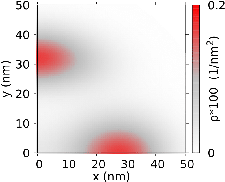
The effects of the electron-electron correlation in the localization of the carriers can be observed in the pair-correlation function plots given in Fig. 5. For these plots we fix the position of one of the electrons (see in Eq. (6)) that is marked by the cross in each panel of Fig. 5. For illustration of the system reaction to the electron position, we fixed one of the electrons slightly off the local density maxima of Fig. 5 near the left (top) edge of the charge distribution in the left (right) column of Fig. 5. For 3 electrons [Fig. 5(a,b)] the conditional probability exhibits two separate maxima. The maxima move once the fixed electron position is changed [cf. Fig. 5(a,b)], which corresponds to the ring-like charge distribution in Fig. 4(c,d). On the other hand, for the probability maxima at the right and bottom edges of the quantum dot stay in the same place when the fixed electron position is changed [Fig. 5(c,d)]. Note that for the charge density produces the pronounced single-electron maxima [Fig. 4(e,f)].

|

|

|

|

|

|

|
For the single-electron islands forming a Wigner molecule in the real space are not observed since the number of local charge maxima is not equal to [Fig.4(c,d)]. The single-electron charge maxima can appear in the real space when the symmetry of the confinement potential is lowered [24] by e.g. an off-center impurity. We use a weak Gaussian perturbation introduced to the confinement potential used in ,
| (9) |
with parameters meV, nm, and nm.
We considered the spin-polarized states at the magnetic field, near the ground-state symmetry transition from even to odd parity, below 4 T for Fig. 3(c). The blue lines in Fig. 6 present the energy levels of a clean system adopted from Fig. 3(c). The red lines show the energy levels for the perturbed system. The off-center Gaussian impurity opens avoided crossings between the energy levels [Fig. 6] which for the clean potential correspond to opposite parity.
The charge density for the ground (excited) state of is given in Fig. 7(a-c) for the magnetic field that is swept across the avoided crossing. The charge density outside the avoided crossing [Fig. 7(a,c,d,f)] produces four maxima along the ring-like charge distribution, which deviates from the point symmetry due to the potential. At the avoided crossing the wave functions from otherwise crossing levels mix. In the ground state [Fig. 7(b)] three well-separated single-electron islands appear and the charge density is low at the center of the perturbation (). The excited state [Fig. 7(e)] at the avoided crossing produces a Wigner molecule that is rotated by the angle. In this sense, the even and odd-parity states for a clean potential can be understood as superposition of states producing Wigner crystallization in real space with two equivalent but rotated charge distribution. This result for three electrons in circular potential but anisotropic effective mass is similar to the ones found previously for isotropic mass but anisotropic confinement potential [79, 80].
III.1.2 5-electron system in the circular quantum dot

|

|

|

|
The five-electron systems has a more complex structure than systems with two to four electrons due to two charge distributions that appear in the low energy spectrum [see Fig. 3(e)]. In ground-state at we find 6 nearly degenerate energy levels: a odd-parity doublet slightly below even parity quartet. The charge density in all these energy levels is organized in the Wigner molecule form that is plotted in Fig. 8(a) with one central electron island and four others shifted off the center of the QD forming a cross-like structure that we will denote as (1,4). The near degeneracy of the ground-state is a counterpart of the four-electron ground-state for , where the Wigner molecule is also found. For five electrons the first excited energy level at is a even parity doublet also with (1,4) charge distribution. In several higher excited energy levels the states at the energy of meV the charge density is organized in a ring-like structure with four charge density maxima without the single-electron islands. We will denote this structure as (0,4). In higher excited levels the states with (1,4) and (0,4) structure interlace on the energy scale. For T the ground-state becomes fully spin-polarized [Fig. 3(e)] and the (0,4) structure [Fig. 8(b)] appear in the ground-state. Above 1.7 T the spatial parity of the ground-state change from odd to even and the (1,4) structure [Fig. 8(c)] re-appears in the ground-state. In presence of both types of states near the ground-state – with and without single-electron islands in the laboratory frame – the spectrum contains the features of both (ground-state near degeneracy at ) and symmetry transformations at higher field as for .
The (0,4) state for five electrons has a similar character as the three-electron ground-state. For three electrons the charge density is a superposition of two equivalent configurations one being an inversion of the other. The five-electron charge configurations with the (0,4) state correspond to the superposition one or two electrons at the right/left ends of the charge density near line. One of the two equivalent structures for five electrons can be observed in the pair correlation function plot of Fig. 8(d) for one of the electrons fixed at point (-29.4 nm,0).
III.2 A linear confinement
We discuss two perpendicular orientations of the elongated quantum dot to study the interplay of the potential and effective mass anisotropies.

|

|

|

|

|

|

|

|

|

|

|

|

|
III.2.1 Confinement along the zigzag direction
The spectra for the potential of Fig. 1(d) with the confinement potential elongated along the axis, i.e. in the direction where the effective mass is larger, are given in Fig. 9. The numbers given in Fig. 9(a) near the energy levels at (for and the parity with respect to inversion along the and axes of the eigenstates are definite). The first excitation within , the direction of thinner confinement, occurs 3 meV above the ground state (see the energy level marked by (1,0) in Fig. 9(a)) above 5 states excited in the direction. For (Fig. 9(b)) the singlet-triplet ground state the degeneracy is nearly perfect at . For the state remains two-fold degenerate with spin-singlet and spin-triplet energy levels that coincide in energy. The separation of the electron charges [Fig. 10(a)] is complete, and the system is effectively equivalent to a pair of electrons in a double quantum dot with vanishing tunnelling between the dots, which produces a vanishing exchange energy [19, 81, 82]. The ground-state degeneracy at is also obtained for (Fig. 9(c)). The Wigner crystallized charge density of the three-electron system at is shown in Fig. 10(b). Parity has no significant impact on energy once the electron charges are separated and the energy levels are two-fold degenerate with respect to parity. Low-energy spin-polarized states occur only in the odd parity.
For the ground state at is only close to the degeneracy (Fig. 9(d)) with the even parity ground state at . The spin polarization occurs only in even parity states. The structure of the low-energy spectrum is similar to the one found for the circular quantum dot [Fig. 3(e)] with even-odd parity splitting of energy levels reduced almost to zero.
The results of Fig. 9(c,d) for indicate that for () the low-energy spin-polarized energy levels occur only with the odd (even) parity symmetry. This is in agreement with Ref. [16] that indicated that in 1D Wigner molecules for or with integer the low-energy spin-polarized state has the spatial parity that agrees with the number . Note that for in the circular potential [Fig. 3(c)], for which the Wigner molecules were not formed in the real-space charge density, both odd and even parity spin-polarized states appear in the ground state for a range of magnetic field.
III.2.2 Confinement along the armchair direction

|

|

|

|
For the rectangular gate of Fig. 1(a) with the longer side oriented along the direction, the electron mass along the dot is light and in the transverse direction the mass is heavy. For the preceding subsection with confinement along the zigzag direction [Fig. 9(a)], several lowest energy single-electron states correspond to the same – ground state – energy level of the quantization in the direction perpendicular to the quantum dot axis. For the confinement along the armchair direction, the large mass allow the states with excitations in the direction perpendicular to the confinement axis to appear low in the energy spectrum [Fig. 11(a)]. The first single-electron state excited in the transverse direction is the second excited energy level in Fig. 11(a) (see the energy level described by (0,1)). From this point of view, the system deviates from the quasi 1D confinement, which should be characterized by a large number of excitations along the quantum dot below the energy when the first transverse excitation occurs. However, the charge density of the -electron states is elongated along the direction (see Fig. 10(d,e,f)). The lifting of the even-odd degeneracy is observed in the spectrum for and [Fig. 11(b,c)]. A lower value of allows for a non-negligible electron tunneling between the single-electron islands (cf. the charge density in between the single-electron maxima for and in Fig. 10(a,d) and Fig. 10(b,e)), thus lifting the degeneracy at . Near , the spectrum for (Fig. 11(d)) has a distinctly different character than for the zigzag confinement (Fig. 9(d)) and for the circular confinement [Fig. 3(e)]. In both preceding cases the electrons were separated in the single electron islands [Fig. 4(e,f), Fig. 10(c)]. The ground state charge density for the armchair confinement possesses two single-electron islands at the ends of the dot and a lower but more extended central maximum [Fig. 10(f) for T and Fig. 10(i) for T]. The charge densities of the two central electrons do not separate into single-electron islands. The effect can be attributed to both a large value of that allows the states excited in the direction to contribute to the interacting states and a small value of which makes the formation of the single-electron islands along the direction more expensive in terms of the kinetic energy.
Fig. 10(g,h) shows the spin-resolved pair correlation function for one of the electron positions fixed in the point marked by the cross for T. Fig. 10(g) (Fig. 10(h)) corresponds to the electron distribution with the same (opposite) spin as the fixed electron spin. The electrons at the central maximum of the charge distribution [Fig. 10(f)] possess opposite spin. Note that, with the electrons of the extreme ends of the dots, separated from the central density island, the system at acquires a singlet / triplet spectral structure (Fig. 11(d)) similar to the one for the two-electron system in the circular quantum dot (Fig. 3(b)) – the central two-electron system governs the form of the low energy part of the spectrum.
IV Discussion
The systems confined in quantum dots weakly coupled to electron reservoirs are studied with the transport spectroscopy using the Coulomb blockade phenomenon [83, 54]. In the Coulomb blockade regime, the flow of the current across the dot is stopped when the chemical potential of the confined -electron is outside the transport window defined by the Fermi levels of the source and drain. For a small voltage drop between the reservoirs, the position of the chemical potential can be very precisely determined. The chemical potential is defined by the ground state energies of systems with and electrons [83, 54]. The ground-state energy crossing in the electron system produces -shaped cusps in the charging line as a function of the external magnetic field for the -th electron added to the confined system, while the ground-state transitions for the system produces -shaped cusps. Transport spectroscopy allows reconstruction of the energy spectra with a precision of the order of a few eV [84]. The results presented above indicate that the formation of the Wigner molecule in the laboratory frame leads to a near degeneracy of the ground state near . The larger the electron separation in the single-electron charge islands, the closer the degeneracy at . The ground state becomes spin-polarized at low magnetic field and no further ground-state transitions are observed. The systems without the Wigner molecular charge density undergo a number of ground-state transitions that also appear at higher magnetic field. The transport spectroscopy technique can also be used for detection of the excited part of the spectra when the corresponding energy level enters the transport window [83, 84]. Detection of a dense set of levels near the ground state can be used as a signature of Wigner molecule formation [11, 10].
V Summary and conclusions
We have studied the system of a few electrons in an electrostatic quantum dot confinement induced within a phosphorene layer. A version of the configuration interaction approach dealing with the strong electron-electron interaction effects has been developed. We indicated formation of Wigner molecules with single-electron islands separated in the real space in a system of realistic yet small size. In circular quantum dots, Wigner crystallization in the laboratory frame occurs due to the lowered Hamiltonian symmetry with the anisotropy of the electron effective mass. The Wigner molecules appear in the laboratory frame when the distribution of the single-electron islands is consistent with the Hamiltonian symmetry. For circular quantum dots we found Wigner molecules for 2 and 4 electrons but not for 3 electrons i.e. the conditions for the Wigner crystallization are not directly determined by the mean electron-electron distance. For 5 electrons in the circular confinement two forms of the charge density with or without single-electron islands appear in the ground-state depending on the value of the external magnetic field. Formation of the Wigner molecules in a quasi-1D confinement calls for orientation of the confinement potential with longer axis along the zigzag direction since larger effective mass promotes the single-electron islands localization and the smaller armchair mass supports the quasi 1D confinement. We studied the spectra for both circular and elongated quantum dots to find the signatures of the Wigner crystallization in real space. The systems with single-electron islands forming Wigner molecules in the laboratory frame are characterized by near degeneracy of the ground state at followed by spin polarization in low magnetic field and an energy gap between the nearly degenerate ground state and excited states. These features are missing for systems that do not form single-electron islands. Resolution of these signatures is within the reach of transport spectroscopy techniques.
Acknowledgments
This work was supported by the National Science Centre (NCN) according to decision DEC-2019/35/O/ST3/00097. Calculations were performed on the PLGrid infrastructure.
Appendix
Single-electron eigen-states with , and

|

|

|

|

|

|

|

|

|

|

|

|

|

|

|

|

|

|

|

|

|

|

|

|

|

|

|
Figure 2 presents the convergence of the CI method the single-electron Hamiltonians , and using the bare QD potential , the potential with the central repulsive Gaussian () and the reduced potential , respectively. The low-energy single-electron wave functions are plotted in Fig. A12 for the three Hamiltonians starting from the ground-state in the first row, and the subsequent excited states presented in the lower panels of Fig. A12. The seven lowest-energy states have the same character for all Hamiltonians only with states for (central column of plots) and (right column) covering a larger area than the ones for , which turns out to speed-up the convergence of the CI method for the system of size increased by the strong electron-electron interaction.
Choice of the computational box
The CI method uses the single-electron wave functions that are obtained with the finite difference approach in a finite computational box with the boundary conditions of vanishing wave function at the edges of the box. The edges of the box form effectively an infinite quantum well that has to be chosen large enough to contain the few-electron system without perturbation to the low-energy states. The influence of the size of the box on the results is given in Fig. A13 for the circular quantum dot. For the circular quantum dot we use the square grid of points of the spacing of where is the radius of the computational box and we take . The red (black) line in Fig. A13 shows the ground-state energy for (). The growth of the energy for small is due to the finite-size effect with the quantum well ground state changing as . For calculations for the radius of nm is large enough while for is has to be taken as large as nm.
Spectra without the spin Zeeman interaction
A striking difference in the energy spectra states with or without the Wigner molecule in the ground state is revealed for the circular potential once the spin Zeeman interaction is removed. This is illustrated in Fig. A14 which reproduces the data from Fig. 3 for . The systems with Wigner form of the charge density, i.e. the single-electron islands in the charge density), (Fig. A14(a)) and (Fig. A14(c)) contain a nearly degenerate ground state with energy levels of different parity that interlace in increasing . The separation of the electron charges in the separate, weakly coupled, maxima produces a small energy difference due to the parity, which is similar to the nearly degenerate ground state for identical, weakly coupled quantum dots. The single electron islands are formed by a relatively strong electron-electron interaction and the weakness of the electron tunnelling between the islands can be deduced from the charge density plots of Fig. 4(a,b) and Fig. 4(e,f) for and . In both cases, the bunch of energy levels of the ground state is separated by a distinct energy gap from the excited states.
For [Fig. 8(b)] the parity of the ground state changes in growing as for even but the spacing between the even and odd parity energy levels near the ground state is much larger than for even and no energy gap is observed between the nearly degenerate ground state and the rest of the spectrum.


|
References
- [1] E. Wigner, Phys. Rev. 46, 1002 (1934).
- [2] D.S. Fisher, B.I. Halperin, and P.M. Platzman, Phys. Rev. Lett. 42, 798 (1979).
- [3] T. Smolenski, et al. Nature 595, 53 (2021).
- [4] H. Li. et al. Nature 597, 650 (2021).
- [5] G. W. Bryant, Phys. Rev. Lett. 59, 1140 (1987).
- [6] K. Jauregui, W. Haeusler, and B. Kramer, Europhys. Lett. 24, 581 (1993).
- [7] R. Egger, W. Haeusler, C. H. Mak, and H. Grabert, Phys. Rev. Lett. 82, 3320 (1999).
- [8] I. Shapir, A. Hamo, S. Pecker,C. P. Moca, O. Legeza,, G. Zarand, and S. Ilani, Science 364, 870 (2019).
- [9] A. Diaz-Marquez, S. Battaglia, G.L. Bendazzoli, S. Evangelisti, T. Leininger, and J. A. Berger, J. Chem. Phys. 148, 124103 (2018).
- [10] S. Pecker, F. Kuemmeth, A. Secchi, M. Rontani, D. C. Ralph, P. L. McEuen, and S. Ilani, Nat. Phys. 9, 576 (2013).
- [11] J. Corrigan, J.P. Dodson, H. Ekmel Ercan, J.C. Abadillo-Uriel, B. Thorgrimsson, T.J. Knapp, N. Holman, T. McJunkin, S.F. Neyens, E.R. MacQuarrie, Ryan H. Foote, L.F. Edge, M. Friesen, S.N. Coppersmith, and M.A. Eriksson, Phys. Rev. Lett. 12, 127701 (2021).
- [12] M. Modaressi, and A.D. Guclu, Phys. Rev.B 95, 235103 (2017)
- [13] C. Yannouleas and U. Landman, Phys. Rev. Lett. 82, 5325 (1999).
- [14] S. M. Reimann, M. Koskinen, and M. Manninen, Phys. Rev. B 62, 8108 (2000).
- [15] A. V. Filinov, M. Bonitz, and Y. E. Lozovik, Phys. Rev. Lett. 86, 3851 (2001).
- [16] B. Szafran, F. M. Peeters, S. Bednarek, T. Chwiej, and J. Adamowski, Phys. Rev. B 70, 035401 (2004).
- [17] C. Ellenberger, T. Ihn, C. Yannouleas, U. Landman, K. Ensslin, D. Driscoll, and A. C. Gossard Phys. Rev. Lett. 96, 126806 (2006).
- [18] S. Kalliakos, M. Rontani, V. Pellegrini, C. P. García, A. Pinczuk, G. Goldoni, E. Molinari, L. N. Pfeiffer, and K. W. West, Nat. Phys. 4, 467 (2008).
- [19] J.C. Abadillo-Uriel, B. Martinez, M. Filippone, and Y.-M. Niquet, Phys. Rev. B 104, 195305 (2021).
- [20] E. Cuestas, P.A. Bouvrie, and A.P. Majtey, Phys. Rev. A 101 033620 (2020).
- [21] D. Vu and S. Das Sarma Phys. Rev. B 101, 125113 (2020).
- [22] M. Reimann and M. Manninen, Rev. Mod. Phys. 74, 1283 (2002).
- [23] Jianyun Zhao, Yuhe Zhang, and J. K. Jain, Phys. Rev. Lett. 121, 116802 (2018).
- [24] C. Yannouleas and U. Landman, Rep. Prog. Phys. 70, 2067 (2007).
- [25] H. Liu, A.T. Neal, Z.Zhu, Z. Luo, X. Xu, D. Tomanek, and P.D. Ye, ACS Nano 8, 4033 (2014).
- [26] L. Li, Y. Yu, G. J. Ye, Q. Ge, X. Ou, H. Wu, D. Feng, X. H. Chen, and Y. Zhang, Nat. Nanotechnol. 9, 372 (2014).
- [27] S. Fukuoka, T. Taen, and T. Osada, J. Phys. Soc. Jpn. 84, 121004 (2015).
- [28] M. Akhar, G. Anderson, R.Zhao, A. Alruqi, J.E. Mroczkowska, G. Sumanasekera, J.B. Jasinski, npj 2D Mater Appl 1, 5 (2017).
- [29] R. Schuster, J. Trinckauf, C. Habenicht, M. Knupfer, and B. Büchner, Phys. Rev. Lett. 115, 026404 (2015).
- [30] J. Qiao, X. Kong, Z.X. Hu, F. Yang, W. Ji, Nat. Commun. 5, 4475 (2014).
- [31] A. N. Rudenko and M. I. Katsnelson, Phys. Rev. B 89, 201408(R) (2014).
- [32] A. N. Rudenko, S. Yuan and M. I. Katsnelson, Phys. Rev. B 92, 085419(R) (2015).
- [33] P. Faria Junior, M. Kurpas, M. Gmitra, and J. Fabian, Phys. Rev. B 100, 115203 (2019).
- [34] X. Zhou, , W.K. Lou, D. Zhang, F. Cheng, G. Zhou, and Chang, K. Phys. Rev. B 95, 045408 (2017).
- [35] B. Szafran, Phys. Rev. B 101, 235313 (2020).
- [36] M. Lee, Y.H. Park, E.B. Kang, A. Chae, Y. Choi, S. Jo, Y.J. Kim , S.J. Park, B. Min, T.K. An, J. Lee, S.I. In, S.Y. Kim, S.Y. Park, I. In, ACS Omega 2, 7096 (2017).
- [37] Z. Sun, H. Xie, S. Tang, Y. Xue-Fang, G.Zhinan,J. Shao, H. Zhang, H. Huang, H. Wang, and P.K. Chu, Angewandte Chemie 127, 11688 (2015).
- [38] M. Wang, Y. Liang, Y. Liu, G. Ren, Z. Zhang, S. Wu, and J. Shen,Analyst 143, 5822 (2018).
- [39] R. Gui, H. Jin. Z. Wang, and J. Li, Chem. Soc. Rev. 47, 6795 (2018).
- [40] V. A. Saroka, I. Lukyanchuk, M. E. Portnoi, and H. Abdelsalam, Phys. Rev. B 96, 085436 (2017).
- [41] H. Abdelsalam, V.A. Saroka, I. Lukyanchuk, and M.E. Portnoi, J. App. Phys. 124, 124303 (2018).
- [42] F. X. Liang, Y. H. Ren, X. D. Zhang, and Z. T. Jiang, J. App. Phys. 123, 125109 (2018).
- [43] L. L. Li, D. Moldovan, W. Xu, and F.M. Peeters: Phys. Rev. B 96, 155425 (2017).
- [44] L. Li, Y. Yu, Q. Ge, X. Ou, H. Wu, D. Feng, X. H. Chen, and Y. Zhang, Nat. Nanotechnol. 9, 372 (2014).
- [45] D. He, Y. Wang, Y. Huang, Y. Shi, X. Wang, and X. Duan, Nano Lett. 19, 331 (2019).
- [46] X. Li, Z. Yu, X. Xiong, T. Li, T. Gao, R. Wang, R. Huang, and Y. Wu, Sci. Adv. 5, eaau3194 (2019)
- [47] N. Gillgren, D. Wickramaratne, Y. Shi, T. Espiritu, J. Yang, J. Hu, J. Wei,X. Liu, Z. Mao, K. Watanabe, and T. Taniguchi, 2D Materials 2, 011001 (2014).
- [48] D. He, Y. Wang, Y. Huang, Y. Shi, X. Wang, and X. Duan, Nano Lett. 19, 331 (2019).
- [49] X.Li, Z. Yu, X. Xiong, T. Li, T. Gao, R. Wang, R. Huang, and Yanqing Wu, Sci. Adv. 5 eaau3194 (2019).
- [50] L. Li, F.Yang, G.J. Ye, Z. Zhang, Z. Zhu, W. Lou, X. Zhou, L. Li, K. Watanabe, T. Taniguchi, and K. Chang, Nat. Nano. 11, 593–597 (2016).
- [51] G. Long, D. Maryenko, S. Pezzini, S. Xu, Z. Wu, T. Han, J. Lin, C. Cheng, Y. Cai, U. Zeitler, and N. Wang, Phys. Rev. B 96, 155448 (2017).
- [52] G. Long, D. Maryenko, J. Shen, S. Xu, J. Hou, Z. Wu, W.K. Wong, T. Han, J. Lin, Y. Cai, R. Lortz, and N. Wang, Nano Lett. 16, 7768 (2016).
- [53] J. Yang, S. Tran, J. Wu, S. Che, P. Stepanov, T. Taniguchi, K. Watanabe, H. Baek, D. Smirnov, R. Chen, and C. N. Lau, Nano Lett. 18, 229 (2018).
- [54] R. Hanson, L. P. Kouwenhoven, J. R. Petta, S. Tarucha, and L. M. K. Vandersypen, Rev. Mod. Phys. 79, 1217 (2007).
- [55] Y. Sajeev and N. Moiseyev, Phys. Rev. B 78, 075316 (2008).
- [56] N. A. Bruce and P. A. Maksym, Phys. Rev. B 61, 4718 (2000).
- [57] H. Saarikoski and A. Harju, Phys. Rev. Lett. 94, 246803 (2005).
- [58] R. Egger, W. Hausler, C. H. Mak, and H. Grabert, Phys. Rev. Lett. 82, 3320 (1999).
- [59] A. Secchi and M. Rontani, Phys. Rev. B 82, 035417 (2010).
- [60] F. Salihbegovic, A. Gallo, and A. Grueneis, Phys. Rev. B 105, 115111 (2022).
- [61] R. M. Abolfath and P. Hawrylak, J. Chem. Phys. 125, 034707 (2006).
- [62] X. Hu and S. Das Sarma, Phys. Rev. A 64, 042312 (2001).
- [63] F. Yang, Z. Zhang, N.Z. Wang, G.J. Ye, W. Lou, X. Zhou, K. Watanabe,T. Taniguchi, K. Chang, X.H. Chen, and Y. Zhang, Nano Letters, 18, 6611 (2018).
- [64] T. Thakur and B. Szafran, Phys. Rev. B 105, 165309 (2022).
- [65] P.E. Faria Junior, M. Kurpas, M. Gmitra, and J. Fabian, Phys. Rev. B 100, 115203 (2019).
- [66] M. Governale and C. Ungarelli Phys. Rev. B 58, 7816 (1998).
- [67] S. Bednarek, B. Szafran, K. Lis, and J. Adamowski Phys. Rev. B 68, 155333 (2003).
- [68] B. Szafran, Phys. Rev. B 104, 235402 (2021).
- [69] R. C. Ashoori, H. L. Stormer, J. S. Weiner, L. N. Pfeiffer, K. W. Baldwin, and K. W. West, Phys. Rev. Lett. 71, 613 (1993).
- [70] A. Szabo and N.S. Ostlund, Modern Quantum Chemistry (Dover, Mineola, NY, 1996)
- [71] Luke W. Bertels, Harper R. Grimsley, Sophia E. Economou, Edwin Barnes, Nicholas J. Mayhall, arXiv:2207.03063, ”Symmetry breaking slows convergence of the ADAPT Variational Quantum Eigensolver
- [72] R. Ahlrichs, H. Lischka, and V. Staemmler, J. Chem. Phys. 62, 1225 (1975).
- [73] P. J. Fasano, C. Constantinou, M. A. Caprio, P. Maris, and J. P. Vary Phys. Rev. C 105, 054301 (2022)
- [74] E.R. Davidson, Rev. Mod. Phys. 44, 451 (1972).
- [75] Benedikt B. Brandt, Constantine Yannouleas, and Uzi Landman, Nano Letters, 15 7105 (2015).
- [76] P.-O. Löwdin, Phys. Rev. 97, 1474 (1955).
- [77] For the circular potential of Fig. 1(a) the optimal parameters for , 4 and 5 electrons are equal to (4 meV, 35 nm), (8 meV, 35 nm) and (10 meV, 40 nm), respectively.
- [78] C. Yannouleas and U. Landman, Phys. Rev. B 105, 205302 (2022).
- [79] Yuesong Li, Constantine Yannouleas, and Uzi Landman Phys. Rev. B 76, 245310 (2007).
- [80] Constantine Yannouleas, Benedikt B Brandt, and Uzi Landman, New J. Phys. 18, 073018 (2016).
- [81] G. Burkard, G. Seelig, and D. Loss Phys. Rev. B 62, 2581 (2000).
- [82] J. R. Petta, A. C. Johnson, J. M. Taylor, E. A. Laird, A. Yacoby, M. D. Lukin, C. M. Marcus, M. P. Hanson, and A. C. Gossard, Science 309, 2180 (2005).
- [83] Kouwenhoven L.P., Marcus C.M., McEuen P.L., Tarucha S., Westervelt R.M., Wingreen N.S. (1997) Electron Transport in Quantum Dots. In: Sohn L.L., Kouwenhoven L.P., Schön G. (eds) Mesoscopic Electron Transport. NATO ASI Series (Series E: Applied Sciences), vol 345. Springer, Dordrecht.
- [84] A. Fuhrer, S. Luescher, T. Ihn, T. Heinzel, K. Ensslin, W. Wegscheider, and M. Bichler, Nature 413, 822 (2001).