Wholesale Market Participation of DERA:
Competitive DER Aggregation
Abstract
We consider the aggregation of distributed energy resources (DERs) by a profit-seeking DER aggregator (DERA), participating directly in the wholesale electricity market and constrained by the distribution network access. We propose a competitive DER aggregation that maximizes the DERA’s profit subject to that each customer of the DERA gains no less surplus and pays no higher energy cost than that under the regulated retail tariff. The DERA participates in the wholesale electricity market as virtual storage with optimized generation offers and consumption bids derived from the DERA’s competitive aggregation. Also derived are DERA’s bid curves for the distribution network access and DERA’s profitability when competing with the regulated retail tariff. We show that, with the same distribution network access, the proposed DERA’s wholesale market participation achieves the same welfare-maximizing outcome as when its customers participate directly in the wholesale market. We empirically evaluate how many DERAs can survive in the long-run equilibrium. Numerical studies also compare the proposed DERA with existing benchmarks on surpluses of DERA’s customers and DERA profits as functions of the DER adoption level and the distribution network access.
Keywords
distributed energy resources and aggregation, behind-the-meter distributed generation, demand-side management, net energy metering, competitive wholesale market.
I Introduction
We address open problems in the direct participation of distributed energy resource aggregators (DERAs) in the wholesale electricity market operated by regional transmission organizations and independent system operators (RTOs/ISOs), under the general framework in FERC order 2222 [2]. We focus on the aggregation strategy of a profit-seeking DERA, whose industrial, commercial, and residential customers have competing service providers, such as their incumbent regulated utilities. The central theme of this work is to develop profitable and competitive aggregation strategies to attract and retain customers. By competitive aggregation, we mean that the benefits of the DERA customers must be no less than those offered by service provider benchmarks. An example of such a benchmark is the incumbent utility or a community choice aggregator (CCA) adopting net energy metering (NEM) policies, offering strong incentives to prosumers with behind-the-meter (BTM) DERs [3, 4, 5]. A major barrier to DERA’s entrance to direct wholesale market participation is having an aggregation strategy and a participation model to make DER aggregation a profitable venture[6].
Currently, there are no existing techniques and analyses supporting profitable competitive aggregation. The technical challenge is twofold. First, the DERA plays a dual role in the aggregation process: an energy supplier to its customers on the retail side and a producer/demand on the wholesale side. Its aggregation strategy must consider retail competition and overall revenue adequacy in wholesale market participation. To this end, a DERA needs to derive profit-maximizing bids and offers from its competitive DER aggregation strategy.
Second, competitive aggregation requires the DERA to offer more attractive pricing than the regulated utility. Note that DERA’s customers are interested in not only the cost-benefit tradeoff but also the pricing rule stability. Examples of unstable pricing are two-part pricing from Griddy [7] and Amber [8] defined by the wholesale spot price and a connection charge. Although Griddy’s aggregation is competitive to regulated utility tariffs, its customers face a 100-fold price increase during the extreme winter event of Uri in 2021.
I-A Related work
There is growing literature on DER aggregation and wholesale market participation models that broadly fall into two categories. One is through a retail market design operated by a distribution system operator (DSO) [9, 10], an aggregation/sharing platform [11, 12], or an energy coalition such as CCA [13, 14, 15]. For the most part, these works do not consider a profit-maximizing DERA’s active participation in the wholesale market. In particular, in [9, 10, 11], the DSO or an aggregation platform participates in the wholesale markets with the aggregated net demand (or possibly net production), treating the wholesale market as a balancing resource.
Our approach belongs to the second category of DER aggregations, where profit-seeking DERAs aggregate both generation and flexible demand resources, participating directly in the wholesale market with bid/offer curves. To ensure secure distribution network operation, DERA obeys the allocated distribution network access limit (or operating envelope [16]), rather than considering the computationally expensive network power flow constraints. Within the framework of FERC order 2222, this type of DER aggregation has the potential to improve the overall system efficiency and reliability.
Although the notion of competitive DER aggregation has not been formally defined, two prior works have developed competitive aggregation solutions in [13, 17]. In [13], Chakraborty et al. consider DER aggregation by a CCA, where the authors provide an allocation rule that offers its customers competitive services with respect to the regulated utility.
Most relevant to our work is the DERA’s wholesale market participation method developed by Gao, Alsheheri, and Birge [17] where the authors consider a profit-seeking DERA aggregating BTM distributed generations (DGs) and offering its aggregated generation resources to the wholesale market. In particular, the Gao-Alshehri-Birge (GAB) approach achieves a social surplus equal to that achievable by customers’ direct participation in the competitive wholesale market. In other words, GAB approaches the most economically efficient participation model. A significant difference between [17] and this paper is that we formulate a general competitive aggregation problem that includes the regulated utility. In achieving DERA’s profit maximization, our DER aggregation and market participation models are different from [17].
The approach proposed in [17] follows the earlier work of Alshehri, Ndrio, Bose, and Başar [18] where a Stackelberg game-theoretic model is used. Both approaches assume that the DERA elicits prosumer participation with an optimized (one-part or two-part) price, and the prosumer responds with its quantity to be aggregated by the DERA. The real-time wholesale market price is reflected by the variable price in [7, 8, 17]. Such a variable price conveys low but volatile wholesale prices directly to customers. To protect customers from price spikes in the real-time wholesale price, some methods like price caps [19] have been proposed. As for the wholesale market participation model of DERA, quantity bid is adopted in [17], price-quantity bid in [18, 16], and virtual power plant in [20], with which we have the same assumption that the DERA centrally schedules customers’ consumption.
I-B Summary of results, contributions, and limitations
In our previous work [1], we develop the first profit-maximizing competitive DER aggregation for a DERA to participate in the wholesale market. In this paper, we further explore the price stability, profitability, market efficiency, and long-run equilibrium for the competitive DER aggregation, especially under the distribution network access limits.
First, we propose a DER aggregation approach based on a constrained optimization that maximizes DERA surplus while providing higher surpluses than that offered by a competing aggregation model. In particular, we are interested in aggregation schemes that are competitive with the regulated utility rates such as NEM X,111NEM X, proposed in [21] is an inclusive parametric model that captures key features of the existing and proposed NEM tariff models. with which a customer can make cost-benefit comparisons in her decision to become a customer of the DERA. We show that such a competitive DER aggregation, despite that the aggregation involving real-time wholesale locational marginal price (LMP), has an energy cost no greater than NEM X. This implies the proposed DER aggregation mechanism ensures price stability regardless of the volatility of the wholesale market LMP, a property missing in Griddy’s pricing model [7]. Meanwhile, we establish the profitability of DERA when competing with NEM X.
Second, we propose a virtual storage model for DERA’s wholesale market participation compatible with the practical continuous storage facility participation considered by ISOs [22, 23] under FERC order 841. The DERA bidding curve is derived from the closed-form solution of the proposed DERA model. While the aggregation optimization explicitly involves wholesale market LMP, the virtual storage bidding curves do not require forecasting of LMP. We show that the proposed DERA wholesale market participation results in market efficiency equal to what is achievable when DERA’s customers participate directly in the wholesale market.
Finally, we derive the benefit function of DERA over distribution network injection and withdrawal access limits. DERAs compete in the distribution network access auction proposed by [24] to acquire network access and we empirically evaluate the number of surviving DERAs in the long-run competitive equilibrium. Additionally, we present a set of numerical results, comparing the surplus distribution of the proposed competitive aggregation solution with those of various alternatives, including the regulated utility. Among significant insights gained are the higher social surplus, customer surplus, and DERA surplus achievable in the proposed competitive DERA model, when compared to other alternatives.
A few words are in order on the scope and limitations of this paper. First, the losses in distribution systems are not considered. Second, the contingency cases where DSO rejects cleared bids and offers from DERA for reliability concerns [2] are neglected. Under the access limit allocation framework proposed in [24], reliability concerns of DER aggregation are already satisfied under normal operating conditions. Lastly, although the proposed competitive aggregation offers higher benefits to DERA customers, it does so with a discriminative payment function, which might raise some equity concerns.
| : | consumption bundle of customers. |
|---|---|
| : | consumption bundle’s upper and lower limits. |
| : | distribution network injection and withdrawal access limits. |
| : | BTM single and aggregated DG. |
| : | competitiveness constant for benchmark prosumer surplus. |
| : | total number of prosumers. |
| : | payment function of the aggregated customer. |
| : | import rate, export rate, and fixed charges of NEM X. |
| : | wholesale locational marginal price (LMP). |
| : | aggregated net injection quantity of DERA. |
| : | total surpluses of DERA and its aggregated prosumers. |
| : | prosumers surplus under tariff NEM X. |
| : | aggregated supply function. |
| : | prosumer utility function for energy consumption. |
| : | prosumer marginal utility function. |
I-C Paper organization and notations
In Sec. II, we summarize the DER aggregation model and its main interactions. The problem of competitive DER aggregation is formulated in Sec. III where we derive the optimal aggregation solution. Sec. IV and Sec. V consider DERA’s wholesale market participation and its bidding strategies in the distribution network access auction, respectively. Numerical simulations are presented in Sec. VI. Sketch proofs are relegated in the appendix.
A list of major designated symbols is shown in Table I. The notations used here are standard. We use boldface letters for column vectors as in . In particular, is a column vector of all ones. The indicator function is denoted by , which equals to 1 if , and 0 otherwise. represents the set of all nonnegative real numbers. represents the set of integers from 1 to , i.e., .
II DER Aggregation Model
A DERA aggregates resources from its customers and coordinates with the DSO for power delivery to the wholesale market operated by ISO/RTO. Following the DERA interaction model proposed in [24], we focus on the DERA-DSO-ISO/RTO interfaces (a)–(c), as shown in Fig. 1. Since a DERA uses DSO’s physical infrastructure for power delivery between its customers and the wholesale market, it is essential to delineate the financial and physical interactions at these interfaces. Sec.II-A–Sec.II-C below describe the three interfaces (a)–(c).

II-A DERA and its customers at interface (a)
We assume the DERA aggregates resources in a retail market from residential, commercial, and industrial customers who have the option of being served by a regulated utility. Under a single-bill payment model, each customer settles its payment for consumption and compensation for production with the DERA. The DERA deploys an energy management system (EMS) with direct controls of the customer’s BTM generation and flexible demand resources, such as rooftop PV, HVAC, water heaters, and EV chargers.222The direct control in [20] is implemented through cloud-based platforms. The DERA optimizes the customer’s BTM resources under competitive aggregation optimization and provides the customer with a cost-benefit comparison with the NEM benchmark offered by the incumbent public utility. See Sec. III for details.
II-B DERA and RTO/ISO at interface (b)
In this paper, we focus on DERA’s participation in the energy market based on a virtual storage model compatible with the continuous storage facility participation model [22]. See Sec. IV for the construction of bid/offer curves. To this end, the DERA submits offer/bid curves or self-scheduled quantity bids. The DERA may participate in both the day-ahead and real-time markets, although here we focus only on the real-time energy or energy-reserve market participation. The DERA may also deploy its own DG and storage capabilities to mitigate aggregation uncertainties. The strategy of incorporating DERA’s own resources in the overall DER aggregation will be discussed in future research.
II-C DERA and DSO at interface (c)
We consider the DERA-DSO coordination model developed in [24] where the DERA acquires access limits at buses in the distribution network operated by a DSO. DERA’s willingness to pay for network access is explained in Sec.V. In particular, after the access limit auction or a direct bilateral contract with DSO, the DERA must aggregate DER from its customers in such a way that abides by the injection and withdrawal constraints set by the allocated access limits, i.e., (1d), in the real-time operation. That way, DERA’s aggregation has no effect on the operational reliability of the DSO under nominal operating conditions,333The contingency conditions can be considered by out-of-market coordination, or by extending the network access allocation in [24]. avoiding DSO intervention on ISO dispatch of DERA’s aggregation.
III Competitive DER Aggregation
This section formulates the optimal competitive aggregation and analyzes the properties of the optimal solution when competing with the incumbent utility’s NEM X. Our DER aggregation is built on the deregulated retail market. For example, in Texas and New York,444Here are hyperlinks for energy providers options in Texas and New York. customers can choose their electricity suppliers based on electricity rate and services. We consider heterogeneous prosumers owning all energy consumptions and DG devices. After joining a DERA, prosumers grant device access to DERA for measurements and control.
III-A Closed-form solution for competitive DER aggregation
We consider a DERA aggregating over point of aggregations (PoAs) in the distribution network. We define PoAs555A diagram illustrating PoA is in Fig. 2 of [24]. as the main buses with higher voltages in the distribution network, which can be recognized with main substation information [25]. For simplicity, we illustrate the single time interval aggregation model of one prosumer at each PoA,666The model (1) can also be applied to the representative customer at each PoA. Such a representative customer exists when utility functions of all customers at each PoA have the Gorman form [26, P119]. and all PoAs face one zonal LMP. This model can be extended to two general cases: (i) the aggregation with multiple time intervals, whose empirical analysis is shown in Sec. VI-E, and (ii) the aggregation with multiple prosumers at one PoA and the device-level control, shown in Appendix VIII-G.
The DERA solves in real-time for the consumption bundle of all customers and their payment functions from the following optimization.
| (1a) | ||||
| subject to | ||||
| (1b) | ||||
| (1c) | ||||
| (1d) | ||||
where the objective represents the DERA profit given real-time BTM DG and LMP .
To attain customers in the energy aggregation, we design the -competitive constraint (1b) to ensure that the surplus of prosumer under DERA is higher than the benchmark prosumer surplus , whose detailed setting is explained in Sec. III-B. This is the criteria for a rational customer, seeking surplus maximization, to join a DERA. Otherwise, a rational prosumer has the incentive to leave DERA and switch to the benchmark service provider for a higher customer surplus. The prosumer utility for consuming energy is represented by the function , which is assumed to be concave, nonnegative, nondecreasing, continuously differentiable, and . We assume the consumer utility function is given. In practice, utility functions can be computed with parametric[21] or nonparametric[27] methods.
The rest of the constraints in (1) impose operation limits. and are prosumer consumption limits. The DERA has corresponding injection and withdrawal access limits at the PoAs of distribution networks, represented respectively by exogenous parameters with details in Sec. V.
Theorem 1 (Optimal DERA scheduling and payment).
Given the wholesale LMP , the optimal consumption bundle of the customer at PoA , and its payment are given by
| (2a) | ||||
| (2b) | ||||
where is the inverse demand curve for customer given price , and the marginal utility function is .
The sketch of proof is provided in Appendix VIII-D, following the convexity and Karush-Kuhn-Tucker (KKT) conditions of (1). This optimal solution has two noteworthy characteristics. First, the optimal consumption in (2a) is only a function of the wholesale LMP when DERA purchases enough injection and withdrawal access at the PoA . Note also the difference between the optimal consumption schedule in (2a) and those in [18] where the optimally scheduled consumption always depends on the anticipated LMP and forecast of BTM DG. Second, (1) finds a Pareto efficient allocation that maximizes the surplus of the DERA, subject to the constraint that the aggregated customer has the given level of surplus . Similar optimization and the Pareto efficient allocation are also analyzed in [28, P602] for first-degree price discrimination. The payment function can be realized by a two-part tariff, which is explored by GAB, although it unidirectionally aggregates BTM DG [17]. Overall, such a closed-form solution allows DERA to apply simple dispatch and pricing policies over massive aggregated households.
III-B Properties of DERA competitive with NEM X
We analyze the profitability of DERA and the energy consumption cost of aggregated prosumers for the optimal DERA aggregation competitive with a regulated NEM tariff parameterized by the retail (consumption) rate , the sell (production) rate , and the connection charge . Assume without loss of generality. Denote the -th prosumer surplus under NEM X to be , whose computation depends on the DG generation and network access limits (formulation provided in Appendix VIII-A). We can set the benchmark prosumer surplus , to obtain competitive aggregation over the DSO’s NEM-based aggregation with the same distribution network access.777Customers owning DERs switch from NEM X to DERA for higher consumer surplus, granting DERs control to DERA upon joining.
The -competitive constraint in (1b) has significant implications on pricing stability, despite that the aggregation is based on real-time LMP. Price stability means the price and payment faced by customers cannot go randomly high, for which a counterexample is the real-time LMP. Because the NEM tariff has price stability, achieving a finite customer payment regardless of the wholesale LMP fluctuation, an aggregation mechanism competitive with the NEM tariff must also be stable. The proposition below formalizes this intuition.
Proposition 1 (Average cost of consumption).
Assume , then the average total cost of consumption for all DERA’s customers is always upper bounded by , i.e., , .
The sketch of proof is provided in Appendix VIII-B. Such price stability comes directly from the -competitive constraint, which enforces a lower bound for customer surplus and thus naturally limits the maximum customer payment. Note that the two-part pricing of Griddy [7] is not a stable pricing mechanism because the retail rate is tied directly to the real-time LMP.
In the -competitive constraint (1b), controls the surplus distribution among DERA and its aggregated prosumers. A larger rebates more benefits to prosumers and incentivizes prosumers to join DERA, although it increases the deficit risk of DERA. DERA has to set properly to avoid deficits while attracting prosumers. In the proposition below, we guarantee DERA’s profitability when is bounded above and all prosumers’ surpluses are nonnegative under NEM X.
Proposition 2 (Profitability of DERA).
For , assume and . Denote , if ; and , if . Then, , and the profit of DERA is nonnegative when .
The sketch of proof is provided in Appendix VIII-C. So, if NEM X is not crediting BTM DG of prosumer at a higher production rate than wholesale LMP, our aggregation method is profitable when competing with NEM X to attain customers. In practice, happens since many states including California are setting the export rate at the avoided cost rate, which is, in many cases equivalent to the wholesale LMP [29], to mitigate cross-subsidies [6, 4].
IV DERA Wholesale Market Participation
Virtual storage model [23] allows DERA to participate in the wholesale electricity market with bi-direction. This means DERA can submit a combination of supply offers and demand bids, purchasing aggregated consumption (as charging the virtual storage) and selling its aggregated production (as discharging). The virtual storage model for DERA is adopted by most system operators in electricity markets [22].
IV-A Offer/bid curves of DERA in energy markets
As a virtual storage participant in the real-time energy market, the DERA is either self-scheduled or scheduled by ISO/RTO according to its bids and offers. This work focuses on developing price-quantity bid/offer curves that define DERA’s willingness to produce and consume.888For the quantity bid, one would forecast the LMP, and compute the optimal net production with defined in (2a). In a competitive market, such curves are the marginal cost of production and the marginal benefit of consumption derived from the optimal DERA decision in Theorem 1.
Let be the aggregated quantity to buy (when ) or sell (when ) for the DERA and be the wholesale market LMP. Let be the BTM DG aggregated by DERA. In a competitive market, a price-taking DERA participant bids truthfully with its aggregated supply function given by
| (3) |
where is defined in (2a). Note that the inverse of the DERA supply function defines the offer/bid curves of the DERA. By submitting a bidding curve as virtual storage, DERA does not need to forecast LMP. Note also that the supply function depends on the aggregated BTM generation , which is not known to the DERA at the time of the market auction. In practice, can be approximated by using historical data or vis the Law of Large Numbers involving independent prosumers or via the Central Limit Theorem for independent and dependent random variables [30].
IV-B Market efficiency with DERA participation
We now establish that the DERA’s participation in the wholesale market achieves the same social welfare as that when all profit-maximizing prosumers participate in the wholesale market individually under certain conditions. We assume the wholesale market is competitive, where all participants are price takers with truthful bidding incentives.
Consider a transmission network with buses. Without loss of generality, we assume PoAs at the distribution network are connected to each bus of the transmission network and all prosumers are aggregated by the proposed DERA model. Denote as the aggregated prosumer utility function at the -th PoA of the -th transmission network bus, and are respectively the BTM DG generation and energy consumption for the prosumer, is the bid-in benefit function of the flexible demand at bus when consuming , and is the bid-in cost function for the generator at bus when producing . For simplicity, we assume each transmission bus has bids from one elastic demand and one generator. Denote , , as the parameter for the DC power flow model of the transmission network, and the line flow limit for branches of the transmission network.
Lemma 1 (Wholesale market clearing with DERA).
When prosumers participate in the wholesale market indirectly through the proposed DERA model with offer/bid curve (3), the social welfare is the optimal value of
| (4a) | ||||
| subject to | ||||
| (4b) | ||||
| (4c) | ||||
| (4d) | ||||
| (4e) | ||||
The sum of the DERA surplus and prosumers’ surpluses, denoted by , can be computed by
| (5) |
Proof of this Lemma in Appendix VIII-E relies on showing that pricing and dispatch results from (4) are at the bidding curve of DERA, i.e., (3). With the optimal dual variable for the power balance constraint (4b) and for the line flow limit (4c), the market clearing LMP over buses is defined by , where . The aggregated prosumer utility in (5), and constraints for energy consumption and distribution network access in (4d) (4e) come from DERA’s offer/bid (3).
As for the prosumer’s direct participation in the wholesale market, we know that a price-taking prosumer at PoA and bus constructs her offer/bid curves by solving the following surplus maximization problem with the given LMP :
| (6) |
where because we assume prosumers participating in the wholesale market directly are facing the same network injection and withdrawal access limits at each PoA for the fairness of comparison. So, the bid/offer curve of the prosumer at PoA and bus is
| (7) |
where takes the same definition as that in (2a).
Let and be, respectively, the optimal social welfare and prosumers’ surplus when all prosumers directly participate in the wholesale market. The following theorem is parallel to [17], although we have different aggregation methods, under the model that the DERA (and prosumers) submits its bids and offers to the wholesale electricity market.
Theorem 2 (Market efficiency).
When all prosumers directly participate in the wholesale market, the market clearing result can be computed by (4), , and
The sketch of proof is provided in Appendix VIII-F, which relies on the fact that the proposed DERA has its bidding curve (3) equal to the sum of the prosumer’s bidding curve in (7). From this, we can establish that the wholesale market clearing problem with the direct participation of all prosumers has the same market-clearing results as (4).
Although the proposed DER aggregation model only focuses on DERA’s profit maximization in the objective (50), the competitive constraint (1b) aligns the aggregated prosumer’s surplus maximization with DERA’s profit maximization. So, the proposed competitive DER aggregation has the incentive to maximize prosumers’ surpluses and get the maximum total surplus that can be split among DERA and its aggregated prosumers. Essentially, DERA acts as a middleman and brings all prosumers to indirectly participate in the wholesale market. Since DERA is profiting from this middleman business, the individual prosumer receives less payment in the indirect wholesale market participation through DERA than from direct wholesale market participation (shown by Fig. 2). This is not unreasonable. After all, individual prosumers cannot participate directly in the wholesale market.
V DERA-DSO coordination
All generation and consumption resources aggregated by DERA need to bypass the distribution network to participate in the wholesale market. The DERA aggregation presented in this work assumes that the aggregated DER at each distribution network PoA is bounded by access limits imposed through the distribution network access limit auction in [24]. A DERA submits a bid curve in this auction representing its willingness to acquire access at PoAs in the distribution system.
We assume that a DERA is a price taker in the access limit auction. Therefore, the bid-in demand curve for network access from the DERA at a particular PoA is the marginal benefit (profit) from having a DER aggregation under the PoA. The maximum expected profit of DERA is given by
where is the maximum DERA profit computed from the optimal value of (1), with the vector of realized renewable generations over all buses and the realized LMP. Note that when participating in the forward network access auction, the BTM DG and LMP are random.
V-A DERA benefit function for distribution network access
The following Proposition provides an expression for the benefit function of DERA, , which can be used as the bid curve of access limits submitted to the auction in [24].
Proposition 3 (Benefit function for network access).
With the DERA profit maximization (1), the expected DERA surplus is
| (8) | ||||
The sketch of proof is provided in Appendix VIII-D. The optimal DERA surplus is decomposed into three terms: the surplus dependent on the withdraw access , the surplus dependent on the injection access , and the surplus independent of the network access . When there are no binding constraints for network access limits, is the optimal consumption of prosumer , defined below (2a); when there are binding access limits, the optimal consumption equals truncated by the distribution network access limits, and DERA’s benefit is modified by or .
In our aggregation model, the optimal DERA benefit is separable across injection and withdrawal access, and across prosumers at different distribution buses. Furthermore, at most one of and can be nonzero, depending upon the renewable generation for prosumer . When , is nonzero and the prosumer at bus is a consumer with binding network withdrawal access constraints; when , is nonzero and the prosumer at bus is a producer with binding network injection access constraints. Related simulation is shown in Sec. VI-D.
V-B Long-run equilibrium for competitive DERA
In a long-run competitive industry, we explore how many DERA can survive. DERAs compete to attract customers, attain distribution network access, and participate in the wholesale market. We assume all DERAs adopt the proposed competitive DER aggregation method. The condition for a competitive long-run equilibrium [31, P193]999In [31], question 4.26 focuses on long-run competitive equilibrium; equations (4.21) and (4.22) focus on long-run monopolistic equilibrium. has two components: (i) the marginal benefit of DERA equals the marginal cost of DSO for providing the distribution network access, and (ii) all DERAs have profits equal to zero, i.e., DERA’s profit in conducting aggregation equals DERA’s payment to acquire distribution network access. Related derivations and simulations are in Sec. VI-E and Appendix VIII-H.
VI Case Studies
We compared the expected surplus distribution of different DER aggregation methods under varying distribution network access limits and BTM DG generations. Under the access limit allocation framework in [24], distribution network reliability concerns are resolved if DERA obeys the allocated distribution network access limit. So the distribution network topology was ignored in the simulation. We also computed the benefit function of DERA to the distribution network access and empirically evaluated the long-run equilibrium of DERA with multi-interval aggregation. The DERA bidding curve to the wholesale market was simulated in our previous paper [1].
VI-A Parameter settings
Assume homogeneous utility function [21] for the aggregated customers, i.e., ,
| (9) |
where . The marginal utility had , for the consumption boundaries.
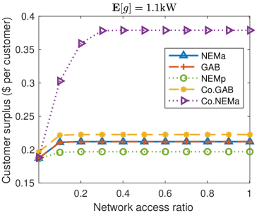
We used NEMa and NEMp to represent the DER aggregation under NEM X when prosumers were active and passive, respectively. Passive customers are not responsive to the retail prices, but active customers will optimize their energy consumption given the retail price and the BTM DG generations. Based on PG&E residential rate, we set for the NEM X. We assumed and the fixed cost of NEM X was covered by extracting fixed payment from DERA, so we simulated with . GAB represented the two-part pricing in [17] which allowed customers to sell BTM DG to the DERA while purchasing energy from its incumbent utility company. Detailed models for NEMa, NEMp, and GAB are provided in Appendix VIII-A. Our DER aggregation method was simulated in Co.NEMa and Co.GAB, competitive to NEMa and GAB respectively. We set at the upper bound in Proposition 2 for Co.NEMa. For Co.GAB, we set to provide 5% more customer surplus than the GAB competitor.
LMP was assumed to be a Gaussian random variable with mean $0.05/kWh and standard deviation (STD) $0.01/kWh, truncated by . The BTM DG generation was assumed to be a Gaussian random variable with STD 0.2 kWh, truncated by . Data sources for the wholesale LMP and BTM DG came from CAISO and Pecan Street Dataport [32], respectively. We sampled 10,000 scenarios for the LMP and BTM DG. At a certain PoA, we analyzed the per-customer level surplus distributions on expectation based on the sample mean of these scenarios.
VI-B Performances with unlimited distribution network access
Four observations below were drawn when all aggregators received plenty of distribution network access.


First, Co.NEMa and Co.GAB were at the Pareto front in Fig. 2 achieving the maximum social surplus as if all prosumers directly participated in the wholesale market without middlemen like DERA. This verified Theorem 2. Note that we computed the Pareto front by adding up surpluses of DERA and customers, omitting surpluses of other units. This was because we adopted the price taker assumption in the wholesale market, thus surpluses of other units stayed the same in different DERA models. The blue dot, named Direct, represented the ideal case that prosumers directly participated in the wholesale market with bidding curve (7). The green rectangular contained aggregation methods achieving less DERA surplus and customer surplus than Co.NEMa, thus dominated by our proposed competitive DER aggregation method. Similarly, the orange rectangular was dominated by its top right corner, Co.GAB. This was because our aggregation methods efficiently participated in the wholesale market with aggregated resources and scheduled the aggregated customers at a consumption level with a higher customer surplus. When the expected BTM DG increased from 1.1kW to 5.1kW, comparing the left and right panels in Fig. 2, we observed the expected social surplus, which was the sum of DERA and customer surpluses, increased, because more BTM DG was sold to the wholesale market.
Second, customers had the highest expected surplus in Co.NEMa and Co.GAB shown by the top of Fig. 3. Passive customers in NEMp had the least surplus because its scheduling had no awareness of DG generation. Customer surpluses almost overlapped in all cases at a low DG adopter ratio with fewer producers, since most aggregation benefits came from BTM DG of producers. When the DG adopter ratio increased, the expected customer surplus increased in all cases.


Third, when DG adopter ratio or the DG generation was low, Co.NEMa and Co.GAB achieved the highest expected DERA surplus, as is shown in the bottom of Fig. 3. When the DG adopter ratio and DG generation were high, GAB achieved the highest DERA surplus because GAB only aggregated producers.101010GAB achieved the Pareto front when all prosumers were producers, e.g. DG adopter ratio equal 100% and kW. Co.NEMa always had DERA profit no less than zero since we chose based on Proposition 2. NEMp and NEMa were completely overlapped when comparing DERA surplus because we set .
Fourth, since NEM X provided a higher surplus to customers with BTM DG, DERAs must commensurately reduce their own profits and share them with the customers to remain competitive with NEM X. Therefore, in most cases of Fig. 3, the expected DERA surplus decreased when the DG adopter ratio increased. However, GAB witnessed an increasing DERA surplus when the DG adopter ratio increased because GAB only aggregated producers.
VI-C Performances with limited distribution network access
Set distribution network access limits for each prosumer by kW and vary the network access ratio from 0 to 1 to analyze the influence of limited distribution network access. First, as is shown in Fig. 4, either Co.NEMa or Co.GAB achieved the highest customer surplus and DERA surplus under a limited network access ratio. Second, when the network access ratio increased, customer surplus increased in most cases except NEMp which passively controlled DG. Third, the DERA surplus in all cases increased when the network access ratio increased. This was intuitive because aggregators needed distribution network access to deliver the aggregated resources and participate in the wholesale market.


VI-D Benefit function of DERA for distribution network access
We computed the bid-in benefit function of the proposed DERA model, i.e., (8), with and 50 prosumer aggregated at a certain PoA. DERA was competing with NEM X and prosumers were passive. We plot the expected benefit of DERA with respect to the injection and withdrawal access in Fig. 5 with varying expected BTM DG generations.
In the left panel of Fig. 5, DERAs with lower expected DG generations had higher benefits and chose higher bid prices to purchase withdrawal access, as shown by the slope of the benefit function. Because, with less BTM DG, DERA relied more on the withdrawn electricity from the network. The slope of the right panel in Fig. 5 showed that DERAs with higher DG chose higher prices for injection access. The benefit function was lower when the DG generation was higher. This counterintuitive phenomenon happened because NEM X provided higher surpluses to customers with higher DG, DERAs must reduce their profits and share them with the customers to remain competitive with NEM X.


VI-E Long-run competitive equilibrium of DERAs
In the long-run competitive equilibrium analysis with multi-interval aggregation of DERs, we assumed 200 DERAs initially existed and computed the expected number of surviving DERAs in the long run. For simplicity, we assumed DERAs were homogeneous and had the same setting as Sec. VI-D. Prosumers had the same expected DG generation created from the 24-hour roof-top solar data in Pecan Street [32].111111Detail DG trajectories and the long-run equilibrium results for single-interval aggregation are shown in Appendix VIII-H, providing intuitions about long-run equilibrium for multi-interval aggregation here. We multiplied the mean of 24-hour DG by to simulate different DG installation capacities and sampled 10,000 random DG scenarios. DERA submitted the benefit function, as in Fig. 5, to acquire hourly distribution network access. Same as [24], the DSO cost function for providing distribution network access was assumed to be the sum of quadratics, with for both the injection and withdrawal access. We multipied DSO’s cost by to simulate different levels of DSO’s costs.
Two observations were drawn from results in Fig. 6. First, when the DG capacity ratio was about 0.4-1.4, all initial 200 DERAs survived because DERAs can internally balance customer demands with its aggregated DG, thus relying and paying less to the network access. This was validated by the yellow dot curve from Fig. 6 (right), which required almost zero network access over 24 hours. Second, when the DG capacity ratio decreased from 0.4 to 0 in Fig. 6 (left), the number of surviving DERA decreased. In this case, DG was lower than the aggregated customers’ consumption, and not all DERAs can survive when competing and paying for the network withdrawal access over 24 hours, shown by the blue solid curve of Fig. 6 (right). In the green dash curve of Fig. 6 (left), DSO’s cost for providing network access was lower, so more DERAs survived than other curves. Similar reasons applied when DG capacity ratio increased beyond 1.4.


VII Conclusions
A major issue facing the realization of FERC order 2222 goals is how can DERAs compete with the lucrative retail programs offered by legacy utility companies. To this end, this paper considers the competitive DER aggregation of a profit-seeking DERA in the wholesale electricity market. As a wholesale market participant, DERA can both inject and withdraw power from the wholesale market. It is shown that the proposed DERA model maximizes its profit while providing competitive services to its customers with higher surpluses than those offered by the distribution utilities. We also establish that the resulting social welfare from DERA’s participation on behalf of its prosumers is the same as that gained by the direct participation of price-taking prosumers, making the proposed DERA aggregation model optimal in achieving wholesale market efficiency. Additionally, we derive two significant optimal price-quantity bids of DERA, of which one is submitted to the wholesale market, and the other to the distribution network access allocation mechanism [24].
An open issue of the proposed aggregation solution is that the payment functions for prosumers are nonlinear and non-uniform. Although each customer is guaranteed to be better off than the competing scheme, two customers producing the same amount may be paid and compensated differently. In other words, the total charge/credits depend not only on the quantity but also on the flexibilities of the demand and constraints imposed by the prosumer. Note that a profit-seeking DERA participating in the wholesale electricity market is not subject to the same regulation as a regulated utility. Such non-uniform pricing is acceptable and has also been proposed in the form of discriminative fixed charges [17, 6].
Acknowledgement
The authors are grateful for the many discussions with Dr. Tongxin Zheng, Dr. Mingguo Hong, and other colleagues from ISO New England. We also benefited from helpful comments and critiques from Dr. Jay Liu and Dr. Hong Chen from PJM.
References
- [1] C. Chen, A. S. Alahmed, T. D. Mount, and L. Tong, “Competitive DER aggregation for participation in wholesale markets,” in Proceedings of the 56th Hawaii International Conference on System Sciences. [Online preprint] arXiv:2207.00290, 2023.
- [2] FERC. (2020) Participation of distributed energy resource aggregations in markets operated by regional transmission organizations and independent system operators, order 2222. 2020. Accessed: June 9, 2024. [Online]. https://www.ferc.gov/sites/default/files/2020-09/E-1_0.pdf.
- [3] M. Birk, J. P. Chaves-Ávila, T. Gómez, and R. Tabors, “TSO/DSO coordination in a context of distributed energy resource penetration,” Proceedings of the EEIC, MIT Energy Initiative Reports, Cambridge, MA, USA, pp. 2–3, 2017.
- [4] A. S. Alahmed and L. Tong, “Integrating distributed energy resources: Optimal prosumer decisions and impacts of net metering tariffs,” SIGENERGY Energy Inform. Rev., vol. 2, no. 2, p. 13–31, Aug. 2022.
- [5] J. Nelson, “Order 2222: Observations from a Distribution Utility,” Southern California Edison (SCE), Tech. Rep., 10 2021.
- [6] S. Borenstein, M. Fowlie, and J. Sallee, “Designing electricity rates for an equitable energy transition,” Energy Institute at Haas working paper, vol. 314, 2021.
- [7] “Real-time wholesale electricity pricing in Griddy,” Accessed: June 9, 2024. [Online]. https://www.energyogre.com/is-realtime-wholesale-pricing-risky, February 2022.
- [8] “Amber wholesale energy price explained,” Accessed: June 9, 2024. [Online]. https://www.youtube.com/watch?app=desktop&v=DckQbwwWPWA and https://www.amber.com.au/electricity, June 2021.
- [9] S. D. Manshadi and M. E. Khodayar, “A hierarchical electricity market structure for the smart grid paradigm,” IEEE Transactions on Smart Grid, vol. 7, no. 4, pp. 1866–1875, 2015.
- [10] R. Haider, D. D’Achiardi, V. Venkataramanan, A. Srivastava, A. Bose, and A. M. Annaswamy, “Reinventing the utility for distributed energy resources: A proposal for retail electricity markets,” Advances in Applied Energy, vol. 2, p. 100026, 2021.
- [11] T. Morstyn and M. D. McCulloch, “Multiclass energy management for peer-to-peer energy trading driven by prosumer preferences,” IEEE Transactions on Power Systems, vol. 34, no. 5, pp. 4005–4014, 2018.
- [12] Y. Chen and C. Zhao, “Review of energy sharing: Business models, mechanisms, and prospects,” IET Renewable Power Generation, 2022.
- [13] P. Chakraborty, E. Baeyens, P. P. Khargonekar, K. Poolla, and P. Varaiya, “Analysis of solar energy aggregation under various billing mechanisms,” IEEE Transactions on Smart Grid, vol. 10, no. 4, pp. 4175–4187, 2018.
- [14] L. Han, T. Morstyn, and M. McCulloch, “Incentivizing prosumer coalitions with energy management using cooperative game theory,” IEEE Transactions on Power Systems, vol. 34, no. 1, pp. 303–313, 2018.
- [15] F. Moret and P. Pinson, “Energy collectives: A community and fairness based approach to future electricity markets,” IEEE Transactions on Power Systems, vol. 34, no. 5, pp. 3994–4004, 2018.
- [16] A. Attarha, M. Mahmoodi, S. M. N. R. A., P. Scott, J. Iria, and S. Thiébaux, “Adjustable price-sensitive DER bidding within network envelopes,” IEEE Transactions on Energy Markets, Policy and Regulation, vol. 1, no. 4, pp. 248–258, 2023.
- [17] Z. Gao, K. Alshehri, and J. R. Birge, “Aggregating distributed energy resources: efficiency and market power,” Manufacturing & Service Operations Management, 2024.
- [18] K. Alshehri, M. Ndrio, S. Bose, and T. Başar, “Quantifying market efficiency impacts of aggregated distributed energy resources,” IEEE Transactions on Power Systems, vol. 35, no. 5, pp. 4067–4077, 2020.
- [19] “What is the energy price cap and how does it affect me?” Accessed: June 9, 2024. [Online]. https://www.nerdwallet.com/uk/personal-finance/what-is-the-energy-price-cap/, April 2023.
- [20] “Turnkey VPPs: Streamlining der management for the decarbonized grid of the future,” Accessed: June 9, 2024. [Online]. https://storage.pardot.com/764473/1680019430TuQTtLtN/230327_Turnkey_VPP_White_Paper.pdf, March 2023.
- [21] A. S. Alahmed and L. Tong, “On net energy metering X: Optimal prosumer decisions, social welfare, and cross-subsidies,” IEEE Transactions on Smart Grid, 2022.
- [22] ISO-NE. (2019) Continuous storage facility participation. Accessed: June 9, 2024. [Online]. https://www.iso-ne.com/static-assets/documents/2019/02/20190221-csf.pdf.
- [23] ——. (2021) Order no. 2222: Participation of distributed energy resource aggregations in wholesale markets. Accessed: June 9, 2024. [Online]. https://www.iso-ne.com/static-assets/documents/2021/07/a7_order_2222.pdf.
- [24] C. Chen, S. Bose, T. D. Mount, and L. Tong, “Wholesale market participation of DERAs: DSO-DERA-ISO coordination,” IEEE Transactions on Power Systems, pp. 1–12, 2024.
- [25] “Italy publishes interactive map of substations for energy communities,” Accessed: June 9, 2024. [Online]. https://www.pv-magazine.com/2023/10/06/italy-publishes-interactive-map-of-substations-for-energy-communities/, October 2023.
- [26] A. Mas-Colell, M. D. Whinston, J. R. Green et al., Microeconomic theory. Oxford university press New York, 1995, vol. 1.
- [27] H. R. Varian, “The nonparametric approach to demand analysis,” Econometrica: Journal of the Econometric Society, pp. 945–973, 1982.
- [28] ——, Price discrimination. Elsevier, 1989, vol. 1.
- [29] “2022 distributed energy resources avoided cost calculator documentation,” Accessed: June 9, 2024. [Online]. https://www.cpuc.ca.gov/-/media/cpuc-website/divisions/energy-division/documents/demand-side-management/acc-models-latest-version/2022-acc-documentation-v1a.pdf, June 2022.
- [30] P. Billingsley, Probability and measure. John Wiley & Sons, 2008.
- [31] G. A. Jehle and P. J. Reny, Advanced microeconomic theory. Pearson, 2011.
- [32] “Pecan street dataport,” Accessed: June 9, 2024. [Online]. https://www.pecanstreet.org/dataport/.
- [33] A. J. Ros, T. Brown, N. Lessem, S. Hesmondhalgh, J. D. Reitzes, and H. Fujita, “International experiences in retail electricity markets,” The Brattle Group: Sydney, Australia, 2018.
VIII Appendix
VIII-A Participation model of prosumers
A prosumer in a distribution system can choose to enroll in a NEM X retail program offered by her utility or a DERA providing energy services. In this context, a summary of short-run analysis over several existing models for the participation of prosumers in the regulated utility and different DERA schemes is presented.
VIII-A1 NEM benchmarks
Considering the benchmark performance of a regulated utility offering the NEM X tariff, we extend the results in [21, 4] and present closed-form characterizations of consumer/prosumer surpluses.
For simplicity, we drop the prosumer index and adopt one representative prosumer. The prosumer’s net consumption is
| (10) |
where is the BTM distributed generation (DG). The prosumer is a producer if and a consumer if .
In evaluating the benchmark prosumer surplus under a regulated utility, we assume that the prosumer maximizes its surplus under the utility’s NEM X tariff with parameter , where is the retail (consumption) rate, the sell (production) rate, and the connection charge. In general under NEM X tariff, and the prosumer’s energy bill for the net consumption is given by the following convex function
| (11) |
The prosumer surplus under NEM with parameter is
For an active prosumer whose consumption is a function of the available DG output , the optimal consumption and prosumer surplus can be obtained by
For the fairness of comparison, we assume the aggregated customer is subject to the same distribution network injection and withdrawal access limits, i.e., , which is the same as that applied to the proposed DERA optimization (1) at all PoAs. So, for the above optimization, the domain is .
The surplus and the consumption of an active prosumer are given by the following equations.
| (12) | ||||
where , , with
| (13) |
and, by solving , we have .
A prosumer is called passive if it decides energy consumption without the awareness of its DG output and the influence brought by NEM X switching among and . The optimal consumption bundle of such a passive prosumer under the NEM X tariff is given by
| (14) |
The total consumption and the surplus of a passive prosumer are given by
| (15) | ||||
| (16) |
In practice, because active prosumer decision requires installing special DG measurement devices and sophisticated control, most prosumers are passive.121212Britain establishes a database for passive customers and encourages the participation of passive customers in the electricity market [33]. In summary, the prosumer surplus under NEM X, is given by
| (17) |
VIII-A2 Two-part pricing in GAB
The optimal DERA two-part pricing scheme is proposed in [17] to aggregate BTM DG productions. The original pricing scheme keeps the customer surplus under DERA competitive with that when the customers directly buy energy from the wholesale market. Here, considering the realistic retail market setting, we revised the DERA pricing model to be competitive with that when the customers directly buy energy from the incumbent utility company under NEM X.
The two-part pricing includes a variable price and a discriminative fixed charge . Prosumers can sell energy to the DERA with price , and buy energy from the energy provider, e.g. the utility company, with the retail rate . In this case, the surplus maximization of prosumer is given by
| (18) |
where , and
With function defined in (13), the optimal energy consumption of DERA computed from the optimization above is given by
where . If prosumer chooses not to sell energy to DERA, the maximum prosumer surplus is given by
To make DERA competitive with the incumbent utility company, we set for the -competitive constraint. That way, the prosumer selling energy to DERA will always have times its surplus under the incumbent utility company with NEM.
The profit maximization of the DERA is
| (19) |
And the optimal pricing from the above optimization is
So, when , the prosumer will be aggregated by DERA for its extra BTM DG generation. Otherwise, the prosumer will stay under the utility company with NEM. And the customer surplus under this two-part pricing has . GAB also needs to set carefully to avoid DERA deficit.
VIII-B Proof of Proposition 1
If , we have
Here, (a) comes from the optimal solution in Theorem 1. (b) relies on the setting that . (c) replies on and the assumption that . (d) comes from the definition of given in (17).131313We ignore the fix charge under NEM X here for simplicity.(e) comes from
| (20) |
which can be derived from the optimality of
If , for passive prosumer, we have
Here,(a) comes from the optimal solution in Theorem 1. (b) relies on the setting that . (c) replies on and the assumption that . (d) comes from the definition of given in (17). (e) replies on and . (f) comes from (20). (g) holds because and .
VIII-C Proof of Proposition 2
Denoting the DERA surplus as , we have
Here, (a) comes from the definition of DERA surplus, which is the objective function of (1)and (b) comes from the optimal solution in Theorem 1. (c) follows the assumption that , representing positive surpluses for all prosumers under NEM X. From Lemma 2 and the upper bound of , we have ,
(c) comes from summing the equation above . ∎
Lemma 2.
Assume NEM X has production price equal to LMP, i.e., , then
| (22) |
Proof: , and are defined in (13).
When , we have
Here, (a) follows the optimality of
| (23) |
where . (b) relies on and . (c) comes from the definition of in (17) and .
When this prosumer is passive and , we have
where (a) follows the optimality of (23), (b) comes from the condition that , and (c) comes from the definition of in (17).
VIII-D Proof of Theorem 1 and Proposition 3
We prove this proposition with Karush-Kuhn-Tucker (KKT) conditions of (1), and the inventory calculation with the optimal solution.
Assign dual variables to (1), we have
| (24) |
The Lagrangian function is
Hence, from KKT conditions of (24), we have,
| (27) |
where * indicates the optimal solution.
Combined with the complementary slackness condition, the first constraint of (24) is always binding with , and the optimal consumption equals to if it falls into the interval . So we have
| (28) |
| (29) |
where .
When , we have . The optimal value can be computed by
When , we have . The optimal value can be computed by
In all other cases, the optimal value is given by the equation below, which is not a function of .
| (30) |
Denote
and
To sum up over all cases, we have
| (31) |
So, the maximum expected profit of DERA is given by
| (32) |
∎
VIII-E Proof of Lemma 1
Add dual variables and merge the energy consumption limits for (4), we have
| (33) |
KKT conditions of the optimization (LABEL:eq:_SS_CCDiPro) gives
| (34) |
where indicates the optimal solution. , is the -th column of the shift factor matrix , and . Replace in LMP with definition , (34) becomes
| (35) |
When , from (35).
When , we have and from the complementarity slackness condition. So (35) becomes
| (36) |
Known that the prosumer utility function is assumed to be concave and continuously differentiable. We have
Similarly, when , we have , , and .
VIII-F Proof of Theorem 2
Because the bidding curve of DERA (3) is the direct sum of the prosumers’ bidding curve (7). So (4) is the market clearing problem when prosumers directly participate in the wholesale market with the bid/offer curve (7). That way, equals the optimal value of (4), which is the same as .
By summing up the optimal prosumer surplus, which is the optimal value of (6), over all buses and PoAs, we get and it equals . ∎
VIII-G Aggregated multiple prosumers at a single PoA
Consider a DERA aggregating heterogeneous prosumers under a single point of aggregation (PoA). Note that under the same PoA, the wholesale LMP is the same. Each prosumer has energy-consuming devices, including lamps, air-conditioners, washers/dryers, heat pumps, and electric vehicles. In real-time, the DERA solves for the consumption bundle of all customers and their payment functions , defined by
from the following optimization
| (43) |
where the optimal objective value is the DERA profit given real-time BTM DG . The first constraint, referred to as the -competitive constraint, ensures that the surplus of prosumer under DERA is higher than the benchmark prosumer surplus when BTM DG has generation . and are consumption limits, and is the utility for the customers. We assume the utility function is concave, nonnegative, nondecreasing, continuously differentiable, additive (i.e., ) across the devices, and . The last constraint is added to limit the injection and withdrawal access at this single PoA with the distribution network injection and withdrawal capacities .
Theorem 3 ( ).
Given the wholesale market LMP , the optimal prosumer payment is given by
| (44) |
And the optimal consumption bundle of prosumer , is
| (45) |
where . We have , , and . The expected DERA surplus is
| (46) | ||||
| where | ||||
Since , we have by the complementary slackness condition.
Let and . Known that dual variables for the inequality constraints are always nonnegative, i.e., , we have .
When , we have , from (43). From the KKT condition, we have
Thus, when , by complementary slackness condition, we have , so
When , we have , so
This gives . Similarly, when , we can show , and . From and the concavity of the utility function,
With the same method, we can show that when , and . And when , and . ∎
VIII-H Details about long-run competitive equilibrium
Here we add details for derivations and parameters in the long-run equilibrium analysis. The long-run equilibrium for single-interval aggregation provides insights into the results in the main text for the multi-interval aggregation.
VIII-H1 Single-interval long-run competitive equilibrium
Denote as the number of aggregated prosumers. In the simulation, we have for each DERA. With the quadratic utility of homogeneous prosumer parameterized by and in (9), the profit of the -th DERA defined in (24) is
| (50) |
where is the aggregated DG generation and is the competitive benchmark for aggregated prosumers. Here, we only derive the case for network withdrawal access and the case for injection access can be similarly computed.
In the competitive market setting for the distribution network access auction, the network withdrawal access price is assumed to be exogenous. DERA conducts its profit maximization by
Similarly, DSO’s optimization is
where is defined as the cost function of DSO for providing the withdrawal access of the distribution network at a certain PoA. For simplicity, we ignore the distribution network reliability constraints in DSO’s optimization.
Denote the equilibrium price and access allocations as . Denote as the total number of homogeneous DERAs we have
| (51) |
showing the total network withdrawal access is partitioned to individual DERAs. The optimality conditions for these optimizations of DERA and DSO give the first condition for the long-run competitive equilibrium:
(i) The marginal benefit of DERA equals the marginal cost of DSO for providing the distribution network access, i.e.,
| (52) |
The second condition for long-run equilibrium gives:
(ii) all DERAs have profits equal to zero, i.e.,
| (53) |
The conditions for the existence of long-run competitive equilibrium are and .
Interestingly, the wholesale LMP does not influence the long-run equilibrium in (54) because the linear cost/benefit induced by LMP can be completely cancelled by the marginal pricing at competitive equilibrium.
VIII-H2 Single-interval long-run competitive equilibrium
We simulated long-run competitive equilibrium for the single interval aggregation by assuming 200 DERAs existed at the beginning and computed the expected number of surviving DERAs in the long run. For simplicity, we assume homogeneous DERA with the same expectation of BTM DG generation. We sampled 10,000 random scenarios of BTM DG. Same as [24], the cost function of DSO when providing distribution network access was assumed to be the sum of quadratics, with for both the injection and withdrawal access at all PoAs.
Three observations were drawn from empirical results in Fig. 7. First, when the expected BTM DG was about 2-5 kW, all initial 200 DERAs survived and the expected net injection access equals zero. It’s because DERA internally balanced customer demands with BTM DG, thus relying less on competing for the injection or withdrawal accesses. Second, with smaller expected BTM DG, homogeneous DERAs competed for the withdrawal access to the distribution network, and less than 10 DERAs survived in the long run; with larger expected BTM DG, DERAs competed for the injection access and less than 3 DERAs survived. Fewer DERAs survived when competing over the injection access because NEM X credited DG imports well, making DERA survival more challenging under high DG generations. Third, with smaller for the DSO’s cost scaling factor, the DERA payment to the network access was lower, thus more DERA survived in the green dash curve.


VIII-H3 Multi-interval long-run competitive equilibrium
By adding the 24-hour time dimension to the network access and BTM DG generation, we can extend the derivation of (50)(51)(52)(53) from single-interval long-run equilibrium to multi-interval long-run equilibrium. Note that the number of DERA is still a scalar applied to all 24 hours. We include the simulation setting and results for the multi-interval aggregation in Sec. VI-E. The solar scenarios used in the simulation are presented in Fig. 8.
