galaxies: general — galaxies: nuclei — galaxies: statistics
Where’s Swimmy?: Mining unique color features buried in galaxies by deep anomaly detection using Subaru Hyper Suprime-Cam data
Abstract
We present the Swimmy (Subaru WIde-field Machine-learning anoMalY) survey program, a deep-learning-based search for unique sources using multicolored () imaging data from the Hyper Suprime-Cam Subaru Strategic Program (HSC-SSP). This program aims to detect unexpected, novel, and rare populations and phenomena, by utilizing the deep imaging data acquired from the wide-field coverage of the HSC-SSP. This article, as the first paper in the Swimmy series, describes an anomaly detection technique to select unique populations as “outliers” from the data-set. The model was tested with known extreme emission-line galaxies (XELGs) and quasars, which consequently confirmed that the proposed method successfully selected 6070% of the quasars and 60% of the XELGs without labeled training data. In reference to the spectral information of local galaxies at 0.05–0.2 obtained from the Sloan Digital Sky Survey, we investigated the physical properties of the selected anomalies and compared them based on the significance of their outlier values. The results revealed that XELGs constitute notable fractions of the most anomalous galaxies, and certain galaxies manifest unique morphological features. In summary, deep anomaly detection is an effective tool that can search rare objects, and ultimately, unknown unknowns with large data-sets. Further development of the proposed model and selection process can promote the practical applications required to achieve specific scientific goals.
1 Introduction
Multiple intensive surveys have successfully unveiled the broad outline of galaxy formation and evolution; however, certain essential factors still remain unidentified (e.g., [Bland-Hawthorn and Gerhard (2016), Kormendy and Ho (2013), Naab and Ostriker (2017), Wechsler and Tinker (2018)]). In addition, we cannot expunge the possibility that we are still missing certain populations and events, referred to as “unknown unknowns”.
Recent studies demonstrate that rare objects such as extreme emission line galaxies (XELGs), low luminosity quasi-stellar objects (quasar), and dual quasars could be the missing pieces in the complete representation of galaxy formation and evolution. In context, XELGs are presumed to be analogs of high- galaxies that provide information regarding the drivers of cosmic reionization (Cardamone et al., 2009; Amorín et al., 2015; Greis at al., 2016; Yang et al., 2017). Additionally, low-luminosity quasars aid in characterizing the relationship between host galaxies and their quasars (Salim et al., 2007; Schawinski et al., 2010; Matsuoka et al., 2014; Trump et al., 2015; Ishino et al., 2020; Li et al, 2021), and dual quasars are supposedly in a late-stage merger and provide information regarding the relationship between mergers and supermassive black hole (SMBH) evolution (Hopkins et al., 2008; Blecha et al., 2018; Silverman et al., 2020; Tang et al, 2021). Further discoveries of rare populations and unknown unknowns would aid in the detailed understanding of galaxy formation and evolution. However, searching for such uncommon sources requires a massive and expensive data-set. Notwithstanding the large data, the efficient collection of such sources is a challenge that prevents us from statistically investigating their detailed characteristics. Therefore, developing a method of an exhaustive search for rare objects and unknown unknowns based on extensive data-sets is quite important.
From the data-set perspective, ongoing and upcoming wide-field deep surveys using large aperture telescopes are currently exploring rare populations on an advanced level. The Hyper Suprime-Cam Subaru Strategic Program (HSC-SSP: Aihara et al. (2018)) is a large survey project, which uses the Hyper Suprime-Cam (HSC: Miyazaki et al. (2018)) operating on the Subaru telescope. The HSC-SSP comprises three layers: wide, deep, and ultradeep; the wide layer covers 1400 deg2 with multicolored images. In comparison to the Sloan Digital Sky Survey (SDSS, York et al. (2000)), the HSC-SSP provides deeper images owing to its larger 8.2-m-aperture mirror and longer exposure periods (Furusawa et al., 2018; Kawanomoto et al., 2018; Komiyama et al., 2018). Such high-quality imaging data enables the detection of faint rare objects (e.g., extremely metal-poor galaxies (XMPGs): Kojima et al. (2020), high-redshift low-luminosity quasars: Matsuoka et al. (2019), gravitationally-lensed objects: Sonnenfeld et al. (2018), dust-obscured galaxies: Toba et al. (2015) ,and high- protoclusters: Harikane et al. (2019)).
From the perspective of methodology, anomaly detection has recently garnered attention in detecting extremely rare sources from large data-sets. Anomaly detection is a technique that is used to identify uncommon features in sources in a given data-set, which are significantly distinct from most of the existing sources, without using any labeled training data; it means the anomaly detection method can detect unknown anomalous objects or more anomalous objects than known objects or assumed templates, which may be missed by supervised classifiers reliant on certain labeled training data or templates. Thus, the anomaly detection does not require large data-sets of the target rare populations in advance. This novel approach has impacted a wide range of fields such as pathogen detection in magnetic resonance images (Baur et al., 2021), diagnoses of amplitude anomalies from seismic waveform data (Zaccarelli, Bindi, and Strollo, 2021), and a search for new particles in particle physics (Nachman, 2020). This method is also useful for searching rare objects and unknown unknowns in astronomical sources in a large data-set. Indeed, based on the big library from the SDSS, various statistical attempts have been made for astronomical anomaly detection, such as Bayesian algorithms (Mortlock et al., 2012), self-organizing maps (Meusinger et al., 2012; Fustes et al., 2013), clustering algorithms (Andrae et al., 2010; Sánchez Almeida and Allende Prieto, 2013), random forest algorithms (Baron and Poznanski, 2017; Hocking et al., 2018), support vector machines (Solarz et al., 2017), and deep generative models (Stark et al., 2018; Margalef-Bentabol et al., 2020). A recent study by Storey-Fisher et al. (2021) applied deep generative model to imaging data from the second data release of the HSC-SSP. However, a majority of the studies elaborated in prior research were experimental, and thus, greater practical scientific applications are desired with anomaly detection methods.
With this motivation, we launched the Swimmy (Subaru WIde-field Machine-learning anoMalY) survey program, which aims at a blind search of extremely unique galaxy populations in large data-sets obtained from the HSC-SSP and the Subaru Strategic Programs with Prime Focus Spectrograph (PFS-SSP, Takada et al. (2014); Tamura et al. (2016)). This paper, as the first of this series, reports the development of a simple anomaly detection model based on machine learning, which was applied on the HSC-SSP multicolor images to detect outlier objects that exhibit anomalous features primarily in the central region of galaxies. The proposed model was tested by employing known quasar and XELG samples. As they respectively host active SMBHs in the centers and emission-line dominant regions, the anomaly detection method can identify such uncommon features as outliers. Unlike prior anomaly detection surveys, this study scientifically examined the physical characteristics of the selected anomaly sources by combining archive data to provide useful information for further development of anomaly detection methods. Such an effort is required for the forthcoming enormous data that would be delivered by the next-generation legacy surveys conducted in the Vera C. Rubin Observatory. The Rubin Observatory will provide us with the largest imaging data-set covering 18 000 and 20 billion galaxies (Ivezić et al., 2019), which is adequately large to detect a anomaly by simple arithmetic, approximately one out of twelve billion.
The remainder of this paper is organized as follows. The data, sample selection, and data construction are described in section 2, after which the machine-learning based anomaly detection model is presented in section 3 along with the selection of the anomaly candidates from the data-set. In section 4, we discuss the physical properties of the detected anomaly objects from spectral data, and lastly the results are summarized in section 5. Throughout this paper, the AB magnitude system (Oke and Gunn, 1983) was adopted, assuming a Kroupa (2001) initial mass function and a flat WMAP7 cosmology, km s-1 Mpc-1, (Komatsu et al., 2011).
2 Data
2.1 HSC-SSP data
This study employs multi-band () imaging data from the S20A internal release of the HSC-SSP (wide layer), which is presently available as the third public data release (HSC-SSP PDR3; Aihara et al. (2021)). All the images were reduced using a dedicated pipeline, hscPipe (Bosch et al., 2018). The HSC-SSP survey field is divided into square degree areas called tracts and further subdivided into square arcmin areas called patches. We excluded the patches with full-width-half-maximum (FWHM) larger than 1.0 arcsec or shallow imaging depth of the bottom 5th percentiles in PSF limiting magnitude in one or more filters. The thresholds of the PSF limiting magnitude were , , , , or . After removing the inferior-quality patches, we obtained images of 815 square degrees.
2.2 Training and test data-set
We restrict our analysis to 49 319 luminous galaxies in the above area that were brighter than 20 mag in the -band cmodel magnitude (composite model; Abazajian et al. (2004); Bosch et al. (2018)) and within a redshift range of –0.2 (figure 1), where spectroscopic redshifts are obtained by looking for counterparts in the SDSS DR15 (Blanton et al., 2017; Aguado et al., 2019; Bolton et al., 2012) and the GAMA DR3 (Baldry et al., 2018; Hopkins et al., 2013; Baldry et al., 2014) with a search radius of 1 arcsec (Aihara et al., 2021). In addition, we removed sources that were prominently affected by nearby stars, cosmic rays, corrupted pixels, or saturated pixels by referring to various flags (is False) stored in the database: pixelflags_edge, pixelflags_interpolatedcenter, pixelflags_saturatedcenter, pixelflags_crcenter, pixelflags_bad, sdssshape_flag, pixelflags_bright_objectcenter, mask_brightstar_halo, mask_brightstar_ghost, and mask_brightstar_blooming (Coupon et al., 2018; Aihara et al., 2021; Bosch et al., 2018). Moreover, the point sources were excluded by imposing psfflux_magcmodel_mag0.2 in the band (see also Strauss et al. (2002); Baldry et al. (2010)).

Subsequently, we categorized the sample into several classes to train and test our selection model. First, we cross-matched the sample with the MPA-JHU catalog (Brinchmann et al., 2004; Kauffmann et al., 2003; Tremonti et al., 2004), which summarizes detailed spectral measurements for the SDSS DR7 spectra (Abazajian et al., 2009) and is useful for constructing training data and investigating the physical properties of anomaly candidates. In the anomaly selection, it is essential to exclude uncommon sources from the training data as many as possible to ensure that the proposed model does not learn outlier features from the training sample. Thus, we established a data-set based on the MPA-JHU catalog, excluding known XELGs, quasars, and AGN candidates. Herein, the XELG galaxies were defined with the observed equivalent width (EW) of either [Oii]3726,3729, H+[Oiii]4959,5007, or H+[Nii]6548,6584, being larger than 100 Å, and 701 sources satisfied this definition. In addition, we detected 23 sources that have a counterpart in the latest quasar catalog (DR16Q v4: Lyke et al. (2020)). The XELG and quasar samples were used to test the performance of the proposed anomaly selection model, as discussed in subsection 4.1. In addition, possible AGN and low-ionization nuclear emission-line regions (LINER) candidates were removed from the training data based on the flag (BPTCLASS ) in the SDSS library, which classifies galaxy spectra using the Baldwin, Phillips, & Terlevich (BPT) diagram (Baldwin et al., 1981; Kauffmann et al., 2003). Based on these selection criteria, we established the training data that amounted to 21 151 (table 1). Again the training data should ideally not contain anomalies; however, the training data may have undetected anomaly objects or unknown unknowns because these selection criteria depended on only the SDSS 1-D spectral data. Additionally, although this study does not delve into the remaining 23 582 spec- sources, they were still adopted for use in anomaly detection as well as the MPA-JHU sample.
Moreover, we constructed color-selected samples without spectroscopic counterparts for a complementary analysis, as detailed in appendix C.
| Data | N |
|---|---|
| galaxies at –0.2 (test data) | 49 319 |
| (1) SDSS MPA-JHU | 25 714 |
| (1-1) Training data | 21 151 |
| (1-2) XELGs | 701 |
| (3) DR16Q quasars | 23 |
| (4) Other spec- (SDSS & GAMA) | 23 582 |
2.3 Preparation of data cubes
For each galaxy, we retrieved an image of pixels ( arcsec2, with a pixel scale of 0.168 arcsec per pixel: the default size in the HSC-SSP) for each of the five broad-bands. Thereafter, we scaled the pixel values to a range of [0, 1] for the proposed deep-learning algorithm. There are various ways of flux normalization such as logarithmic, power-law, or square-root stretches. Although the appropriate selection of a normalization formula for deep learning of galaxy imaging data is still debatable, this research followed the approach by Lupton et al. (1999, 2004) that adopts an inverse hyperbolic sine function (arcsinh). Moreover, the arcsinh stretch has been commonly applied to galaxy images in public engagement programs such as Galaxy Zoo111https://www.zooniverse.org/projects/zookeeper/galaxy-zoo/ (Lintott et al., 2008, 2011; Willett et al., 2013) and GALAXY CRUISE222https://galaxycruise.mtk.nao.ac.jp. More importantly, this technique can avoid color saturation as the pixel values were normalized across color channels, and thus allow the model to interpret local anomalous color features within the galaxy image.

Furthermore, we slightly modified the code for arcsinh normalization written by the HSC-SSP pipeline team333https://hsc-gitlab.mtk.nao.ac.jp/ssp-software/data-access-tools/tree/master/pdr3/colorPostage to create multicolored imagine cubes for the hscMap444https://hsc-release.mtk.nao.ac.jp/hscMap-pdr3/app/, which is accessible on the HSC-SSP database and citizen science program, GALAXY CRUISE. This algorithm was compiled to apply the arcsinh stretch to five broadband images acquired from the HSC-SSP, , where is a cut-out image in each band with a zero-point magnitude of 19 mag. Nevertheless, we scaled the and the band data by 1/1.2 and 1/1.5, respectively, corresponding to the typical flux to the band flux ratios. Such additional scaling aided in improving the balance of normalized fluxes between the broadbands. Otherwise, the proposed anomaly detection model will assign a higher weight to the and the band data, which are shallower than the band data (Aihara et al., 2021). The normalized flux can be calculated as
| (1) |
where , and the original values were used in the hscMap for the scaling parameter, , and the bias parameter, . Moreover, the flux range was limited to [0, 1], defined as follows:
| (2) |
The conducted scaling process and color visualizations based on the three bands of five broadband images are illustrated in figure 2. The standardization using the mean flux over the entire broadband () allows us to avoid color saturation (Lupton et al., 1999). Note that the bands trace the stellar continua of targets at the rest-frame Å, and the and the band fluxes are scaled to the band flux across the board, which causes an unclear color gradient in these three images. For instance, in case there is a strong H line contribution to the band flux, a significant color excess would be detected in the band (section 4). Therefore, all the images were smoothed with a Gaussian kernel prior to flux scaling to match the observed FWHM to 1.0 arcsec, based on the observed information stored in each patch (subsection 2.1).
3 Methodology
3.1 Model description
The denoising convolutional autoencoder (DCAE), which was applied in this study to detect anomalous galaxies, is an autoencoder (AE; Hinton and Salakhutdinov (2006)) equipped with a layer that add noise (Vincent et al., 2008) and Convolutional Neural Networks (CNN; Lecun et al. (1998); Krizhevsky et al. (2012); Lecun et al. (2015)). The AE is a machine-learning model that learns a latent representation of the input data using two Neural Networks (NN): an encoder and a decoder. The encoder with as a parameter vector reduces the dimension of the input image , and represents in a low-dimensional data in the latent space. Subsequently, the decoder with as a parameter vector reconstructs the input data from the encoded data . Thereafter, the two NNs are optimized to minimize the value of the loss function , which is a function that evaluates the success of the learning process using the original data and reproduction data . Upon considering the mean–squared error (MSE) as the loss function, the optimization relation can be expressed as
| (3) |
Prior to encoding, we added noise to the input data using a GaussianNoise layer that added Gaussian noise with a mean value of 0. The standard deviation of the Gaussian noise, , is a hyperparameter, and we adopted (i.e., Gaussian noise with a standard deviation of 2 percent to the max count) through a trial-and-error process as described in appendix A.

Here, we briefly explain how our DCAE model can serve as a platform for anomaly detection. They trained a reproduction model with enormous data by updating the model weight parameters to minimize the loss function (see e.g., Chen et al. (2018); Zimmerer et al. (2018); Baur et al. (2021)). Therefore, the trained model learns the overall structure representation of the training data, but not the uncommon features existing in them. Upon inputting a galaxy with anomalous features to the trained model, the model is unable to appropriately reconstruct those features and produce an image without them. Consequently, the anomaly candidates can be selected by searching objects that manifest large residuals between the original and reconstructed images.
In this study, we adopted TensorFlow (version 2.5.0; Abadi et al. (2016)) and Keras (version 2.5.0; Chollet et al. (2015)) to construct the DCAE model. In the training process, we leveraged the Google Colaboratoy (Bisong, 2019) to expedite the calculations with a GPU environment. The model architecture is illustrated in figure 3. The input images were five-color () images, each containing pixels, as described in (section 2). The encoder contained convolutional layers (Conv2D), batch normalization layers (BatchNormalization; Ioffe and Szegedy (2015)), activation function layers (activation), and max-pooling layers (MaxPooling2D). Convolutional layers spatially slide filters over the images and produce feature maps, and then max-pooling layers take the max values in windows. Batch normalization layers normalize the output of prior units (Conv2D in this study) by every batch, which increases training efficiency and prevents overfitting (Ioffe and Szegedy, 2015). Activation function layers convert outputs of prior units using an activation function that is usually nonlinear and enables complex representations throughout the NN (CNN). The following rectified linear unit (ReLU; Glorot et al. (2011)) was adopted as the nonlinear activation function except the last layer using the sigmoid function:
| (4) |
Through Conv2D and MaxPooling2D layers in the Encoder, the input data dimensions are reduced to in the latent space (figures 3 and 4), wherein denotes the number of channels in the final Conv2D layer within the encoder. Thus, a smaller value provides stronger constraints on the latent representation. We selected as a trial-and-error process (appendix A).

On the other hand, the decoder consisted of Conv2D, BatchNormalization, Activation, and upsampling layers (UpSampling2D). Upsamling layers simply resize the input images by a scale of two. In addition, the ReLU was adopted as the activation function in the activation layers, except for the final layer in which a sigmoid function was applied:
| (5) |
The filter numbers in each Conv2D layer were 8, 32, 64, and 5, respectively (figure 4).
The deep-learning model was trained using the training data prepared in section refs2, and the Adam optimizer (Kingma and Ba, 2014) was employed to adjust the weight parameters of the model and minimize the loss function value. The optimizer updates the weight parameters using the backpropagation algorithm (Rumelhart, Hinton, & Williams, 1986). A learning rate is a scalar that determines how much weight parameters are updated in each step. We trained the model with a learning rate of until a learning epoch of 10, after which it was altered to (referred to as the learning decay technique in the machine-learning training). Figure 4 explains how imaging data of spiral and early-type galaxies were encoded and decoded by our reproduction model. Additionally, the examples of reconstructed images and residuals in the five bands for normal galaxies from the training data, DR16Q quasars, and XELGs (as defined in subsection 2.2) are illustrated in figure 6. Although the proposed model appropriately reconstructed the normal galaxies, we observed significant residuals between the original and reconstructed images for most of the quasars and XELGs. This is because the trained model was not optimized for uncommon color features originating from sources such as nuclear UV radiation in quasars and strong emission lines, as seen in XELGs.
3.2 Selection of anomaly sources
To select objects with large residuals, such as quasars and XELGs, we defined the anomaly score as:
| (6) |
where means a calculation area described below. Thus, represents the MSE standardized by the square of the pixel counts of the reconstructed image, which gives the magnitude of the deviation from the model prediction. In particular, the area over which is calculated can be varied according to the target type of anomaly detection. Because this study aimed to detect anomalies that have uncommon features in the nuclear regions such as quasars and some XELGs, we only used the central circular area with a diameter of 6 pixels as the calculation area , which broadly corresponds to the seeing FWHM (1 arcsec; subsection 2.3). Note that we may not be able to detect XELGs with their emission-line dominant components in the outer regions based on this definition. The most suitable weight data was defined to enable the selection of maximum number of DR16Q quasars and XELGs based on a model with high selection completeness. The model selection procedure is detailed in appendix A. Sigma excess values of for quasars and XELGs are provided in figure 6. The significant improvements in the anomaly scores in most of the DR16Q quasars and XELGs were compared to those of the normal galaxies derived from the training sample.


From the entire sample, we selected 5955 anomaly candidates by imposing the criteria: is in the top-5th percentile corresponding to the or higher excess (refer to figure 5), and the residual flux in the central area is positive in at least one of the , , and bands. Their identification numbers (object_id), sky coordinates in the HSC-SSP PDR3 (Aihara et al., 2021), and anomaly scores are summarised in table 3. Furthermore, examples of the selected anomaly candidates in each filter are represented in figure 7. The most anomalous galaxies in the current sample are discussed in subsection 4.4.
We determined that 61% of the DR16Q quasars and 63.2% of the XELGs satisfy the above-mentioned criteria. In contrast, there exist sources that have sufficiently high anomaly scores but are excluded from selection owing to their negative residual values, e.g., the numbers of those galaxies are 8, 322, and 14 for the , , and bands, respectively. These objects are further discussed in appendix B. Notably, as we evaluate the anomalies using only the central regions (equation 6), the chance projections of the background galaxies such as red galaxies will not affect the selection till they are not present in the central regions.
| band | Test data | DR16Q quasar | XELG | |||
|---|---|---|---|---|---|---|
| (N=49 319) | (N=23) | (N=701) | ||||
| 2461 | (4.990%) | 7 | (30%) | 263 | (37.5%) | |
| 2147 | (4.353%) | 3 | (13%) | 119 | (17.0%) | |
| 2455 | (4.978%) | 9 | (39%) | 282 | (40.2%) | |
| 391 | (0.793%) | 1 | (4%) | 77 | (11%) | |
| 385 | (0.781%) | 2 | (9%) | 51 | (7.3%) | |
| 418 | (0.848%) | 2 | (9%) | 119 | (17.0%) | |
| 86 | (0.17%) | 0 | (0%) | 26 | (3.7%) | |
| Total | 5955 | (12.07%) | 14 | (61%) | 443 | (63.2%) |
| ID | R.A. [deg] | Dec. [deg] | Band | |
|---|---|---|---|---|
| 36411461425187990 | 30.58684 | -5.99814 | (0.00076, 0.00982, 0.00708) | |
| 36411590274208581 | 30.44342 | -6.28742 | (0.03182, 0.00485, 0.00031) | |
| 36415992615686651 | 31.99153 | -6.09370 | (0.05844, 0.00023, 0.00489) | |
| 36416117169733290 | 31.81884 | -6.76016 | (0.00296, 0.00096, 0.00786) | |
| 36416409227512668 | 31.37596 | -5.98973 | (0.05086, 0.00229, 0.00056) | |
| … | … | … | … | … |

4 Discussion
In this section, we initially discuss the selection of quasars and XELGs in subsection 4.1. Thereafter, the counterparts of the anomaly candidates were searched from the AGN catalogs, as described in subsection 4.2, and discuss the physical properties of anomaly candidates in subsection 4.3. Lastly, we discuss the most rare and unique objects in the sample (subsection 4.4).
4.1 Validation with quasars and XELGs
Our method selected 61% of the DR16Q quasars (= 14/23) and 63.2% of the XELGs (= 443/701). As these fractions are much higher than the anomaly fraction over the entire sample, 12.07% (= 5955/49319), the proposed method can preferentially select quasars and XELGs. To evaluate the performance of our anomaly detection method, we compared known quasars and XELGs selected as anomaly sources by the proposed method with the unselected known sources. We focused on radial profiles for quasars and emission-line EWs for XELGs because they are, respectively, the vital features characterizing these two populations. This comparison will assist us in interpreting the kind of features that can be identified by the proposed machine-learning model.
First, the quasars were examined. For ease of explanation, we focused on the quasars that are selected and not selected in a specific band, the band ( and , respectively; see table 2). The original and residual radial profiles for the quasars selected and not selected in the band are presented in figure 8. As compared to the unselected objects, the selected objects exhibit significant nuclear excesses in the residual image. Accordingly, we confirmed that the model can select quasars in cases of sufficiently large band excesses present in the center. As the model was not optimized for the unique color features observed in type-I AGNs and quasars, model reconstructions were generated without the blue (the band) nuclear components, as identified in the residual profiles (figure 8). However, the proposed model could accurately reproduce the band images of the unselected quasars in the band, which exhibited inadequate band excesses, regardless of the clear nuclear components in the band as well as the selected quasars. Note that the quasars and AGNs could be variable objects, and the SDSS spectra were obtained a decade ago. Therefore, certain known quasars could be inactive during the operation of the HSC-SSP (March 2014–January 2020 for HSC-SSP PDR3; Aihara et al. (2021)).

Furthermore, the XELGs were examined by focusing on the EWs of strong emission lines, as their intense emission-line contributions toward the selection band would yield high anomaly scores (see also subsection 4.3 about the redshift dependence of the anomaly selection rate). In addition, the parameters , , and () were defined to quantify the emission-line contributions to the , , and bands, respectively. Herein, denotes the sum of the observed EWs of the strong emission lines in each band. In this calculation, we considered the actual throughput of the corresponding HSC filters (Aihara et al., 2021). Moreover, depending on the spectroscopic redshift of each source, the following emission lines provided in the MPA-JHU DR8 catalog (Brinchmann et al., 2004; Kauffmann et al., 2003; Tremonti et al., 2004) were considered: [Oii]3726,3729, [Neiii]3869, H, [Oiii]4959,5007, H, [Nii]6548,6584, and [Sii]6717,6731.
The cumulative distributions of for the selected and unselected XELGs are presented in figure 9. The selection rates of objects with Å was 90.7% for the band, 84.4% for the band, and 64.4% for the band. Thus, the selection method can appropriately select the XELGs, given that they have prominent emission-line contributions to the target broadband images. More importantly, the high selection rate in the band could be caused by the band excess, which is a relatively uncommon trend in the training data.
Based on these results, we concluded that the proposed model tends to select known rare objects with more anomalous features, specifically, quasars with a larger excess in the residual image and XELGs with intense emission lines. Note that the proposed model is not an identifier only for quasars and XELGs, and thus we do not discuss selection purity of these sources in this paper.

4.2 Evaluation with the Milliquas catalog
In this subsection, the performance of the proposed model is determined based on the AGNs and quasars that were not used in the model training or selection process. For this purpose, we cross-matched our anomaly source sample with the Milliquas (Million Quasars) Catalog v7.2 (Flesch, 2021) that contains all the public AGNs and quasars as on April 30, 2021. Because we used the DR16Q sample in the model selection process, we excluded the DR16Q sample from the sample before matching with the Milliquas catalog. AGNs and quasars in the Milliquas catalog matched with the test data are archived from the SDSS DR16 (Ahumada et al., 2020), the low-redshift AGN catalog by Liu et al. (2019), the 2dF galaxy survey (Colless et al., 2001), the 2dF QSO Redshift Survey (Croom et al., 2004), the Principal Galaxy Catalog (Paturel et al., 2003), the Large Sky Area Multi-Object Fiber Spectroscopic Telescope DR3/DR2 (Dong et al., 2018), the WISE AGN catalog (Secrest et al., 2015), and other papers (Ge et al., 2012; Stalin et al., 2010; Francis et al., 2004; Croom et al., 2009; Lacy et al, 2007; Zhou et al., 2006; Gosset et al., 1997; Appenzeller et al., 1998; He and Chen, 1993; Markelijn et al., 1970; Bauer et al., 2000; Massaro et al., 2009; MacAlpine et al., 1981; Trichas et al., 2012; Trump et al., 2007; Lacy et al., 2013; Akiyama et al., 2015; Esquej et al., 2013; Garilli et al., 2014; Rowan-Robinson et al., 2013; Foltz et al., 1989; Chang et al., 2019).
The number of cross-matched sources within 1 arcsec apertures is summarized in table. 4, where object categories follow the object types given in the Milliquas catalog: an optically core dominated object is labeled as “quasar” and a host dominated object is labeled as “AGN”. In addition, Flesch (2019) claimed that “Type- AGNs” may be contaminated by objects such as normal star-forming galaxies, LINERs, or starburst galaxies.
| Test data∗*∗*footnotemark: | Selected anomalies∗*∗*footnotemark: | ||||
| total | |||||
| (N=49 296) | (2454) | (2144) | (2446) | (5941) | |
| quasar | 23 | 10 | 2 | 7 | 16 |
| Type- AGN | 286 | 62 | 20 | 87 | 130 |
| Type- AGN | 580 | 35 | 11 | 40 | 74 |
| Others†{\dagger}†{\dagger}footnotemark: | 49 | 6 | 5 | 7 | 14 |
| total | 938 | 113 | 38 | 141 | 234 |
The DR16Q sample are excluded.
†{\dagger}†{\dagger}footnotemark:
Objects with quasar-like features, such as BL Lac objects, or quasar candidates.
We determined that the proposed model selected 70% of the quasars and 45.5% of type- AGNs, which are much higher than the anomaly fraction over the entire sample, 12.07% . Thus, these significant fractions suggested that the proposed method preferentially selected the quasar and type- AGN samples. On the contrary, the selection rate of type- AGNs was 12.8% , which was as low as the anomaly fraction. Thus, the proposed method is not advantageous in searching type- AGNs. The lower selection rate of type- AGNs was potentially caused by their smaller impacts on host galaxies in comparison to type- AGNs in the optical regime. Thus, we concluded that an anomaly detection method, once optimized with appropriate test data, would be applicable for a blind search of quasars and type- AGNs.
Next, the bandpass dependence of the selection rate is discussed. For quasars, type- AGNs, and type- AGNs, the selections based on the and bands yield three to five times higher selection rates than those based on the band (table 4). Such high selection rates in the band would be attributed to luminous UV radiation from the accretion disk, while those in the band would be caused by strong H and [Nii] emission lines existing in this band. For the remaining AGN class (“others”), the selection rate was similar among the three bands. In contrast, the relatively lower selection rates in the band could be potentially because of their low ( Å). Notably, the Milliquas catalog is incomplete, and therefore, the above-mentioned AGN fractions may increase upon considering the quasars or AGNs missing in the previous surveys.
4.3 Characteristics of anomaly candidates
Until the previous subsection, we determined that only 14 (from the DR16Q sample) and 234 (from the Milliquas catalog) sources () among the 5955 anomaly candidates bear a counterpart in the currently available quasar and AGN catalogs. We performed complementary analyses to examine the characteristics of all the candidates using literature data in this subsection. This characterization will provide valuable insights toward future improvements of the proposed anomaly detection model.
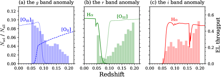
Initially, we examined the redshift dependence of the selection rate shown in figure 10. The selection rate in a given band is defined as the ratio of the number of selected galaxies in that band, , to the number of all galaxies in the test data, . As can be observed from figure 10a, the selection rate in the band decreases with the redshift. This trend can be explained based on the behavior of the throughput of [Oiii] and [Oii] emission lines with the redshift, i.e., the stronger [Oiii] line is captured by the band only at , whereas the weaker [Oii] line is within the band in most of the target redshift range. Such a behavior can also explain an increase in the band selection rate at . Similarly, a spike in the band selection rate at the lowest redshift and a relatively weak redshift bin dependence in the band selection rate are caused by the H line. These results indicated that a significant fraction of the anomaly candidates were selected because of their strong emission line(s) and the selection rate in a given band is strongly dependent on what lines are redshifted into that band.
The influences of on the selection process were further investigated by directly comparing the with the anomaly score for 25 714 galaxies that have EW measurements in the MPA-JHU catalog in figure 11, where the XELG sample is included as well. Again, we found that galaxies with high tend to exhibit high , especially at Å, which indicated that the proposed model preferentially selected the extreme emission-line objects with high anomaly scores. However, figure 11 depicts certain intriguing sources with high but low ( Å). More than half of these outlier objects apparently exhibited artificial-like features, as seen in appendix B, although we cannot expunge the possibility that they have intense line-emission only at the center, which cannot be judged by one-dimensional SDSS spectra captured with the -aperture fibers owing to dilution. Moreover, figure 11 indicates certain galaxies with high ( Å) but low , especially in the band (see also figure 9). However, 70% of these galaxies were selected in other band(s) as well, which implied that their low values can be caused by the flux excess in other bands. For instance, XELGs with low at 0.1–0.2 can be explained based on the intense [Oiii] emission in the band. In such a case, the model may confuse XELGs with red galaxies and thereafter, reproduce their band excesses better than expected.

Furthermore, the dependence of the anomaly score on apparent magnitude was examined. As denotes the square sum of the normalized residuals, it is expected not to be sensitively dependent on apparent magnitude, except for the faint sources bearing low ratios per pixel. The anomaly score is illustrated as a function of apparent magnitude for the entire sample in figure 12. The top 5% and 0.7% (correspond to and ) criteria of for the respective bands are depicted by solid and dashed lines, respectively. In addition, Spearman’s correlation test could not derive any correlation in the three bands, which assures that the proposed method can evaluate anomalies independently of the apparent magnitude in the sample. Note that the anomalies selected in the band tend to be biased toward fainter magnitudes at because the luminous objects with and large tend to exhibit negative residuals. These sources are further examined in appendix B.

Figure 13 indicates the distribution of the galaxies in the MPA-JHU catalog on the SFR– plane. In figure 13, the upper and lower crowds of objects are known to be the star-forming (SF) main sequence and the passive sequence (Brinchmann et al., 2004), respectively. Note that the quasars and AGNs are not plotted because their SFR and would exhibit large uncertainties (e.g., Toba et al. (2018); Toba et al (2021)). In all the bands, the proposed model preferentially selects the galaxies in or above the SF main sequence, as indicated by the adequately small -values () in the Kolmogorov–Smirnov (KS) test. Thus, the result is broadly consistent with the trend that the current method preferentially selected the strong emission-line galaxies. We also confirmed a similar trend as in the GALEX-SDSS-WISE Legacy Catalog 2 (GSWLC-2: Salim et al. (2016); Salim, Boquien, & Lee (2018)), which offers more reliable SFR and measurements than the MPA-JHU catalog because of its multi wavelength coverage from UV to mid-IR. However, significant fractions of anomaly candidates (e.g. 78% in the band selection) that do not appear in this case owing to the absence of counterparts and failures of the SED fit in the GSWLC-2 (see also subsection 4.4), and thus we decided not to use the measurements by the GSWLC-2 in this paper.

The gray and colored histograms in the subplots represent the histograms of and SFR for all anomaly sources, respectively. KS test statistics and its -value are shown in the top and right histograms.
4.4 The most anomalous sources
Ultimately, we examined the emission-line strengths, morphology, and star-formation activities of “the most anomalous sources”, which are defined as with the higher than the (top ). The dashed lines in figures 5, 11, and 12 indicate an excess of . In addition, figures 14 and 15 depict the original multicolored images and the SDSS DR16 (Ahumada et al., 2020) spectra of the most anomalous sources, respectively.
First, the XELGs were determined as dominant in the most anomalous sources. In particular, 71%, 48%, and 65% of the objects over the 3 excess from the MPA-JHU catalog were XELGs in the , , and bands, respectively. These results indicated that the proposed anomaly selection method with the excess, especially in the and bands, facilitated the blind searches of XELGs. However, as certain objects over the 3 excess in the band exhibited a small ( Å; figure 11), the XELG fraction in the band was relatively low.
As can be observed in figure 14, a number of the most anomalous sources exhibited merger-like features or close neighbors. In the former case, we confirmed that the residual images of such galaxies tend to have multiple components even in their residual images, suggesting that they are probably dual AGNs or quasars or have multi-emission-line dominant components. As observed in figure 14, some of the most anomalous sources selected in the band portraying a blue component, such as the blueberry galaxies, also known as XELGs (Yang et al., 2017). Similar trends can be observed in the or bands, as they selected galaxies with a green or red component, respectively. In addition, certain sources with a purple component were caused by the strong emission-line contributions from the [Oiii] (or [Oii]) and H to the and bands, respectively. Such intense emission-line features can be confirmed in their optical spectra, as depicted in figure 15.
The colored diamond plots in figure 13 illustrate the relationship between the SFR and for the most anomalous sources. In all the band, the majority of the most anomalous sources are located above the SF main sequence. Besides, the most anomalous sources tend to be less massive compared to the entire sample. Although some of the most anomalous sources in the band are located in the passive sequence, in appearance they are the artifact-like sources as discussed in appendix B.
We also comment about fractions of the invalid SFR– measurements in the GSWLC-2 for the most anomalous sources (see subsection 4.3). We noticed that % of the most anomalous sources cannot be appropriately fitted with the SED templates in the GSWLC-2 (Salim, Boquien, & Lee, 2018), which are remarkably higher than that of the complete test data, 0.67%. Such a high fraction suggests that the proposed method selected anomalies that exhibited too anomalous photometric colors to apply the SED fitting, owing to extreme emission lines or emission from SMBH, as observed in figure 15. Therefore, specialized templates are required to appropriately derive these physical parameters, which constitute as the in-depth analyses in future research.
Conclusively, the present anomaly candidate sample contained unique populations. Further investigations of such sources will help in the search for interesting objects such as dual quasars, XELGs, or galaxies with unusual merger-like features. Thus, we expect that the application of the proposed deep-anomaly detection method on unprocessed larger data-sets can result in the discovery of extremely unique objects, including unknown unknowns. This aspect was demonstrated by applying the current model on a magnitude-limited color-selected sample without spectroscopic counterparts, as described in appendix C.


5 Conclusion
This paper proposed a method based on machine learning to select galaxies with an anomaly in their central region. Subsequently, the model was applied on 49 319 sources at in the HSC-SSP multiband data. This method evaluated the degree of anomalies using a newly defined parameter, the anomaly score, which is a measure of the light excess in the central region relative to normal galaxies. Overall, we selected 5955 anomaly candidates. As of the quasars, of the type-I AGNs, and of the XELGs in the data-set were selected using this method, new quasars and AGNs that are still unidentified in prior surveys could be present in the remaining candidates.
In addition, the characteristics of the anomaly candidates were discussed to investigate the types of sources selected by the anomaly detection model. For the quasar sample, the selected quasars tended to display larger nuclear residuals in the selection band in comparison to the unselected quasars. Moreover, we determined that galaxies with larger tend to exhibit larger anomaly scores, which indicates that the emission-line dominant sources were preferably selected as anomaly candidates. Moreover, the most anomalous sources exhibiting the highest anomaly scores tended to display very high , and 5070% of them were XELGs. In addition, a number of the most anomalous sources depicted a merger-like feature or were close neighbors. These results demonstrated the superior capability of the proposed anomaly detection method to search for unique populations in the universe.
One limitation of this study is the purity of the training sample. Although the training data should ideally not contain anomalies; however, the training data may have undetected anomaly objects or unknown unknowns because these selection criteria depended on only the SDSS 1-D spectral data. A large survey with integral field units like the Mapping Nearby Galaxies at APO (MaNGA; Bundy et al. (2015)) at may help us restrict and purify the training data in the future. Another solution would be the use of all data as training data without the cleaning by developing our model, which will enable a completely blind anomaly survey.
The major advantage of the proposed anomaly detection method over ordinary methods for searching rare objects is that the current method does not require any model template of targets in advance. Furthermore, the current anomaly detection method is not a classifier or a detector dedicated to specific species such as quasars or XELGs, and therefore, can discover other unique objects, including unknown unknowns. In addition, the proposed model can be flexibly modified to detect anomalies other than those in central regions by adjusting the definition of the anomaly score. Moreover, the application of the anomaly detection model on future large surveys, for instance, PSF-SSP (Takada et al., 2014; Tamura et al., 2016), LSST (Ivezić et al., 2019), Euclid (Amendola et al., 2018), and Roman Space Telescope (Akeson et al., 2019) will provide an excellent opportunity to discover new astronomical sources.
This work is based on data collected at the Subaru Telescope and retrieved from the HSC data archive system, which is operated by Subaru Telescope and Astronomy Data Center at National Astronomical Observatory of Japan. We are honored and grateful for the opportunity of observing the Universe from Maunakea, which has the cultural, historical and natural significance in Hawaii.
We thank anonymous referee for helpful feedback. This work was partially supported by the Summer Student Program (2020) by the National Astronomical Observatory of Japan and the Department of Astronomical Science, The Graduate University for Advanced Studies, SOKENDAI.
The Hyper Suprime-Cam (HSC) collaboration includes the astronomical communities of Japan and Taiwan, and Princeton University. The HSC instrumentation and software were developed by the National Astronomical Observatory of Japan (NAOJ), the Kavli Institute for the Physics and Mathematics of the Universe (Kavli IPMU), the University of Tokyo, the High Energy Accelerator Research Organization (KEK), the Academia Sinica Institute for Astronomy and Astrophysics in Taiwan (ASIAA), and Princeton University. Funding was contributed by the FIRST program from Japanese Cabinet Office, the Ministry of Education, Culture, Sports, Science and Technology (MEXT), the Japan Society for the Promotion of Science (JSPS), Japan Science and Technology Agency (JST), the Toray Science Foundation, NAOJ, Kavli IPMU, KEK, ASIAA, and Princeton University.
This paper makes use of software developed for the Large Synoptic Survey Telescope. We thank the LSST Project for making their code available as free software at http://dm.lsst.org
The Pan-STARRS1 Surveys (PS1) have been made possible through contributions of the Institute for Astronomy, the University of Hawaii, the Pan-STARRS Project Office, the Max-Planck Society and its participating institutes, the Max Planck Institute for Astronomy, Heidelberg and the Max Planck Institute for Extraterrestrial Physics, Garching, The Johns Hopkins University, Durham University, the University of Edinburgh, Queen’s University Belfast, the Harvard-Smithsonian Center for Astrophysics, the Las Cumbres Observatory Global Telescope Network Incorporated, the National Central University of Taiwan, the Space Telescope Science Institute, the National Aeronautics and Space Administration under Grant No. NNX08AR22G issued through the Planetary Science Division of the NASA Science Mission Directorate, the National Science Foundation under Grant No. AST-1238877, the University of Maryland, and Eotvos Lorand University (ELTE) and the Los Alamos National Laboratory.
Funding for the Sloan Digital Sky Survey IV has been provided by the Alfred P. Sloan Foundation, the U.S. Department of Energy Office of Science, and the Participating Institutions. SDSS-IV acknowledges support and resources from the Center for High Performance Computing at the University of Utah. The SDSS website is www.sdss.org.
SDSS-IV is managed by the Astrophysical Research Consortium for the Participating Institutions of the SDSS Collaboration including the Brazilian Participation Group, the Carnegie Institution for Science, Carnegie Mellon University, Center for Astrophysics — Harvard & Smithsonian, the Chilean Participation Group, the French Participation Group, Instituto de Astrofísica de Canarias, The Johns Hopkins University, Kavli Institute for the Physics and Mathematics of the Universe (IPMU) / University of Tokyo, the Korean Participation Group, Lawrence Berkeley National Laboratory, Leibniz Institut für Astrophysik Potsdam (AIP), Max-Planck-Institut für Astronomie (MPIA Heidelberg), Max-Planck-Institut für Astrophysik (MPA Garching), Max-Planck-Institut für Extraterrestrische Physik (MPE), National Astronomical Observatories of China, New Mexico State University, New York University, University of Notre Dame, Observatário Nacional / MCTI, The Ohio State University, Pennsylvania State University, Shanghai Astronomical Observatory, United Kingdom Participation Group, Universidad Nacional Autónoma de México, University of Arizona, University of Colorado Boulder, University of Oxford, University of Portsmouth, University of Utah, University of Virginia, University of Washington, University of Wisconsin, Vanderbilt University, and Yale University.
GAMA is a joint European-Australasian project based around a spectroscopic campaign using the Anglo-Australian Telescope. The GAMA input catalogue is based on data taken from the Sloan Digital Sky Survey and the UKIRT Infrared Deep Sky Survey. Complementary imaging of the GAMA regions is being obtained by a number of independent survey programmes including GALEX MIS, VST KiDS, VISTA VIKING, WISE, Herschel-ATLAS, GMRT and ASKAP providing UV to radio coverage. GAMA is funded by the STFC (UK), the ARC (Australia), the AAO, and the participating institutions. The GAMA website is http://www.gama-survey.org/.
Appendix A Model selection
The proposed model has various hyperparameters such as the dimensionality of the latent space , standard deviation of Gaussian noise, , and number of epochs. One of the challenges in machine learning methods is to select the best hyperparameters, i.e., to select the best model. In this study, we considered the hyperparameters given in table A.
Hyperparameters of the proposed model
parameter
tried values
Latent space dimension
GaussianNoise rate
Epoch number∗*∗*footnotemark:
Iteration†{\dagger}†{\dagger}footnotemark:
{tabnote}
∗*∗*footnotemark: Epoch numbers – were excluded because they were at an insufficient stage of learning.
†{\dagger}†{\dagger}footnotemark: Under the same condition, .
We notice that quantitatively varied results are obtained in different runs because the machine learning model is stochastic. However, the general trends as discussed in section 4 remain unchanged. In addition, we noticed that variations in the results of multiple runs under a fixed set of hyperparameter values were larger than the systematic variations caused by different hyperparameter sets. Therefore, the quantitative evaluation of the hyperparameters is challenging.
Hence, in this study, we decided to train the model several times with fixed and , and subsequently selected the most suitable model among them. These fixed parameters were selected because they provide a relatively lower average loss after ten runs as compared to the additional parameter values in table A. The model training was executed 30 times under the same condition, and the weight data from epochs 10 to 25 was saved. Thereafter, we selected the most suitable weight data from 480 (16 epochs 30 runs) various weight data. Loss values and selection rates calculated with 480 weight parameter sets are summarized in figure 16.

In the model selection, we defined the most suitable weight data as the data for which the sum of the selection rates of known DR16Q quasars and XELGs, (subsection 2.2 for the sample definition) was the highest. All the results presented in the main text, including figures 4 and 6, are based on the model with the most suitable weights.
Appendix B Objects with negative residuals
We examined the objects with a large and a negative residual. These objects were not selected as anomaly candidates and were determined more frequently in the -band. A large with a negative residual in a certain band means a nuclear depression in that band as compared to typical values inferred from the training sample, and therefore, provides significant negative residuals in the nuclear region.
Figure 17 depicts the original, reconstruction, and residual images of sources with a negative residual and the largest in the band. Almost all the sources were determined to have a positive residual in the central region in all the bands except the band. We also observe that flux counts in the band, including background levels, tend to be higher compared to those in the general field, which produce unrealistic green halos as seen in the color images (figure 17). These results indicate that a large with a negative residual in the band is likely due to reduction or technical errors rather than scientific factors, for instance, an error of zero-point correction in the band or saturation in the band in flux normalization. Such artifact-like objects are found in the anomaly candidates as contaminants (subsection 4.4).

Appendix C Further application
In addition, we applied the proposed method to color-selected objects in the local universe without a spectroscopic redshift measurement conducted as a supplemental research. We perform a simple color selection ( and ; see also color selectin in the DEEP2 galaxy redshift survey, Newman et al. (2013)) to remove background sources at as many as possible while keeping a high selection completeness at the target redshift range of –0.2. Although more aggressive color criteria or photo- selection allows a more strict redshift cut, it is not ideal for the deep anomaly detection: as we search for galaxies with anomalous SEDs, such high restrictions may remove potential anomaly candidates in the preselection.
Based on the color selection, the 839 908 of the original samples with mag was reduced to 487 152 sources (figure 18). Given the spec- sample from SDSS DR15 (Blanton et al., 2017; Aguado et al., 2019; Bolton et al., 2012) that consists of the main sample (; Strauss et al. (2002)) and luminous red galaxies (; Eisenstein et al. (2001)), a sampling completeness is 96.5%, a removal rate of or sources is 88.6%, and an outlier fraction in the selected sample is estimated to be 20.9%, respectively.

| ID | R.A. [deg] | Dec. [deg] | Band | |
|---|---|---|---|---|
| 36411444245320355 | 30.59056 | -6.67457 | && | (0.05678, 0.05687, 0.37663) |
| 36411452835251719 | 30.57699 | -6.38626 | (0.00299, 0.00687, 0.02174) | |
| 36411577389302008 | 30.34561 | -6.90563 | (0.16888, 0.00131, 0.00347) | |
| 36411590274208996 | 30.47591 | -6.27652 | (0.00419, 0.08369, 0.00053) | |
| 36411594569174631 | 30.52445 | -6.16192 | (0.00106, 0.00612, 0.02948) | |
| … | … | … | … | … |
Figure 19 represents the most anomalous sources with the top in the color-selected objects, and their identification numbers (object_id), sky coordinates in the HSC-SSP PDR3 (Aihara et al., 2021), and anomaly scores are summarised in table 5. In figure 19, there are many red compact sources unlike our main anomaly samples (figure 14). They could be higher- objects because our machine-learning model has not well learned galaxies. On the other hand, we detect highly blue, green, or purple objects, which would be new candidates of XELGs without spectroscopic confirmations. There are also some clear artifacts as discussed in appendix B. We concluded that the proposed methods are also useful for detecting outliers from the color-selected sample, though further improvements of both training data-set and machine learning model are needed toward practical use.

References
- Abadi et al. (2016) Abadi, M., et al. 2016, arXiv e-prints, arXiv:1603.04467
- Abazajian et al. (2004) Abazajian K., et al. 2004, AJ, 128, 502
- Abazajian et al. (2009) Abazajian, K. N., et al. 2009, ApJS, 182, 543
- Aguado et al. (2019) Aguado D. S., et al. 2019, ApJS, 240, 23
- Ahumada et al. (2020) Ahumada R., et al. 2020, ApJS, 249, 3
- Aihara et al. (2018) Aihara, H., et al. 2018, PASJ, 70, S4
- Aihara et al. (2021) Aihara, H., et al. 2021, arXiv e-prints, arXiv:2108.13045
- Akeson et al. (2019) Akeson, R., et al. 2019, arXiv e-prints, arXiv:1902.05569
- Akiyama et al. (2015) Akiyama, M., et al. 2015, PASJ, 67, 82
- Amendola et al. (2018) Amendola, L., et al. 2018, Living Reviews in Relativity, 21, 2
- Amorín et al. (2015) Amorín, R., et al. 2015, A&A, 578, A105
- Andrae et al. (2010) Andrae, R., Melchior, P., & Bartelmann, M. 2010, A&A, 522, A21
- Appenzeller et al. (1998) Appenzeller I., et al. 1998, ApJS, 117, 319
- Baldry et al. (2010) Baldry, I. K., et al. 2010, MNRAS, 404, 86
- Baldry et al. (2014) Baldry I. K., et al. 2014, MNRAS, 441, 2440
- Baldry et al. (2018) Baldry I. K., et al. 2018, MNRAS, 474, 3875
- Baldwin et al. (1981) Baldwin, J. A., Phillips, M. M., & Terlevich, R. 1981, PASP, 93, 5
- Baron and Poznanski (2017) Baron, D., & Poznanski, D. 2017, MNRAS, 465, 4530
- Bauer et al. (2000) Bauer F.E., et al. 2000, ApJS, 129, 547
- Baur et al. (2021) Baur C., et al. (2021). Medical Image Analysis, 69
- Bisong (2019) Bisong, E. 2019, Google Colaboratory. in Building Machine Learning and Deep Learning Models on Google Cloud Platform (ed. Bisong, E.) 59-64
- Bland-Hawthorn and Gerhard (2016) Bland-Hawthorn, J., & Gerhard, O. 2016, ARA&A, 54, 529
- Blanton et al. (2017) Blanton M. R., et al. 2017, AJ, 154, 28
- Blecha et al. (2018) Blecha, L., Snyder, G. F., Satyapal, S., & Ellison, S. L., 2018, MNRAS, 478, 3056
- Bolton et al. (2012) Bolton, A. S., et al. 2012, AJ, 144, 144
- Bosch et al. (2018) Bosch J., et al. 2018, PASJ, 70, S5
- Brinchmann et al. (2004) Brinchmann, J., et al. 2004, MNRAS, 351, 1151
- Bundy et al. (2015) Bundy, K., et al. 2015, ApJ, 798, 7
- Cardamone et al. (2009) Cardamone, C., et al. 2009, MNRAS, 399, 1191
- Chang et al. (2019) Chang, Y. -L., et al. 2019, A&A, 632A, 77
- Chen et al. (2018) Chen, X., & Konukoglu, E. 2018, arXiv e-prints, arXiv:1806.04972.
- Chollet et al. (2015) Chollet, F., et al. 2015, Available at: https://keras.io
- Colless et al. (2001) Colless M., et al. 2001, MNRAS, 328, 1039
- Coupon et al. (2018) Coupon J., et al. 2018, PASJ, 70, S7
- Croom et al. (2004) Croom S.M., et al. 2004, MNRAS, 349, 1397
- Croom et al. (2009) Croom, S. M. et al. 2009, MNRAS, 392, 19
- Dong et al. (2018) Dong X.Y., et al. 2018, AJ, 155, 189
- Eisenstein et al. (2001) Eisenstein, D. J., et al. 2001, AJ, 122, 2267
- Esquej et al. (2013) Esquej, P., et al. 2013, A&A, 557, 123
- Flesch (2021) Flesch, E. W 2021, arXiv e-prints, arXiv:2105.12985
- Flesch (2019) Flesch, E. W 2021, arXiv e-prints, arXiv:1912.05614
- Foltz et al. (1989) Foltz C.B., et al. 1989, AJ, 98, 1959
- Francis et al. (2004) Francis P.J., Nelson B.O., & Cutri R.M. 2004, AJ, 127, 646
- Furusawa et al. (2018) Furusawa, H., et al. 2018, PASJ, 70, S3
- Fustes et al. (2013) Fustes, D., et al. 2013, A&A, 559, A7
- Garilli et al. (2014) Garilli, B., et al. 2014, A&A, 562, 23
- Ge et al. (2012) Ge J.-Q., et al. 2012, ApJS, 201, 31
- Glorot et al. (2011) Glorot, X., Bordes, A., & Bengio. Y. 2011, In Proc. 14th International Conf. on Artificial Intelligence and Statistics, 315, 323
- Gosset et al. (1997) Gosset, E., et al. 1997, A&AS, 123, 529
- Greis at al. (2016) Greis, S. M. L., et al. 2016, MNRAS, 459, 2591
- Harikane et al. (2019) Harikane Y., et al., 2019, ApJ, 883, 142
- Harris et al. (2020) Harris, C. R., et al. 2020, Nature, 585, 357
- He and Chen (1993) He R., & Chen J.-S. 1993, Ap&SS, 200, 279
- Hinton and Salakhutdinov (2006) Hinton, G. E., & Salakhutdinov, R. R. 2006, Science, 313, 504
- Hocking et al. (2018) Hocking, A., et al. 2018, MNRAS, 473, 1108]
- Hopkins et al. (2008) Hopkins, P. F., Cox, T. J., Kereš, D., & Hernquist, L. 2008, ApJS, 175, 390
- Hopkins et al. (2013) Hopkins A. M., et al. 2013, MNRAS, 430, 2047
- Ioffe and Szegedy (2015) Ioffe, S., & Szegedy, C. 2015, arXiv e-prints, arXiv:1502.03167
- Ishino et al. (2020) Ishino, T., et al. 2020, PASJ, 72, 83
- Ivezić et al. (2019) Ivezić, Z., et al. 2019, ApJ, 873, 111
- Kauffmann et al. (2003) Kauffmann, G., et al. 2003, MNRAS, 341, 33
- Kawanomoto et al. (2018) Kawanomoto, S., et al. 2018, PASJ, 70, 66
- Kingma and Ba (2014) Kingma, D. P., & Ba, J. 2014, arXiv e-prints, arXiv:1412.6980
- Kojima et al. (2020) Kojima, T., et al. 2020, ApJ, 898, 142
- Komatsu et al. (2011) Komatsu, E., et al. 2011, ApJS, 192, 18
- Komiyama et al. (2018) Komiyama, Y., et al. 2018, PASJ, 70, S2
- Kormendy and Ho (2013) Kormendy, J., & Ho, L. C. 2013, ARA&A, 51, 511
- Krizhevsky et al. (2012) Krizhevsky, A., Sutskever, I., & Hinton, G. 2012, In Proc. Advances in Neural Information Processing Systems, 25, 1090-1098
- Kroupa (2001) Kroupa, P. 2001, MNRAS, 322, 231
- Lacy et al (2007) Lacy, M., et al. 2007, AJ, 133, 186
- Lacy et al. (2013) Lacy, M., et al. 2013, ApJS, 208, 24
- Lecun et al. (1998) Lecun Y., et al. 1998, Proc. IEEE, 86, 2278
- Lecun et al. (2015) Lecun, Y., Bengio, Y., & Hinton, G. 2015, Nature, 521, 436
- Li et al (2021) Li, J., et al. 2021, arXiv e-prints, arXiv:2105.06568 https://arxiv.org/abs/2105.06568
- Lintott et al. (2008) Lintott C. J., et al. 2008, MNRAS, 389, 1179
- Lintott et al. (2011) Lintott C., et al. 2011, MNRAS, 410, 166
- Liu et al. (2019) Liu H.-Y., et al. 2019, ApJS, 243, 21
- Lupton et al. (1999) Lupton, R. H., Gunn, J. E., & Szalay, A. S. 1999, AJ, 118, 1406
- Lupton et al. (2004) Lupton R., et al. 2004, PASP, 116, 133
- Lyke et al. (2020) Lyke, B. W., et al. 2020, ApJS, 250, 8
- MacAlpine et al. (1981) MacAlpine G.M., & Williams G.A. 1981, ApJS, 45, 113
- Margalef-Bentabol et al. (2020) Margalef-Bentabol B., et al. 2020, MNRAS, 496, 2346
- Markelijn et al. (1970) Merkelijn J., & Wall J.V. 1970, AuJPh, 23, 575
- Massaro et al. (2009) Massaro E., et al. 2009, A&A, 495, 691
- Matsuoka et al. (2014) Matsuoka, Y., Strauss, M. A., Price, T. N., III, & DiDonato,M. S. 2014, ApJ, 780, 162
- Matsuoka et al. (2019) Matsuoka, Y., et al. 2019, ApJ, 872, L2
- McKinney et al. (2010) McKinney W., et al. 2010, Proc. 9th Python Sci. Conf., 1697900, 51
- Meusinger et al. (2012) Meusinger, H., et al. 2012, A&A, 541, A77
- Miyazaki et al. (2018) Miyazaki, S., et al. 2018, PASJ, 70, S1
- Mortlock et al. (2012) Mortlock, D. J., et al. 2012, MNRAS, 419, 390
- Naab and Ostriker (2017) Naab, T., & Ostriker, J. P. 2017, ARA&A, 55, 59
- Nachman (2020) Nachman, B. 2020, arXiv e-prints, arXiv:2010.14554
- Newman et al. (2013) Newman, J. A., et al. 2013, ApJS, 208, 5
- Oke and Gunn (1983) Oke, J. B., & Gunn, J. E. 1983, ApJ, 266, 713
- Paturel et al. (2003) Paturel, G., et al. 2003, A&A, 412, 45
- Renzini and Peng (2015) Renzini, A., & Peng, Y.-j. 2015, ApJ, 801, L29
- Rowan-Robinson et al. (2013) Rowan-Robinson, M., et al. 2013, MNRAS, 428, 1958
- Rumelhart, Hinton, & Williams (1986) Rumelhart, D. E., Hinton, G. E., Williams, R. J. 1986, Nature, 323, 533
- Salim et al. (2007) Salim, S., et al. 2007, ApJS, 173, 267
- Salim et al. (2016) Salim S., et al., 2016, ApJS, 227, 2
- Salim, Boquien, & Lee (2018) Salim S., Boquien M., Lee J. C., 2018, ApJ, 859, 11
- Sánchez Almeida and Allende Prieto (2013) Sánchez Almeida J., & Allende Prieto C. 2013, ApJ, 763, 50
- Schawinski et al. (2010) Schawinski, K., et al. 2010, ApJ, 711, 284
- Secrest et al. (2015) Secrest, N., et al. 2015, ApJS, 221, 12
- Silverman et al. (2020) Silverman, J. D., et al. 2020, ApJ, 899, 154
- Solarz et al. (2017) Solarz, A., et al. 2017, A&A, 606, A39
- Sonnenfeld et al. (2018) Sonnenfeld A., et al., 2018, PASJ, 70, S29
- Stalin et al. (2010) Stalin, C. S., et al. 2010, MNRAS, 401, 294
- Stark et al. (2018) Stark, D., et al. 2018, MNRAS, 477, 2513
- Storey-Fisher et al. (2021) Storey-Fisher, K., et al. 2021, arXiv e-prints, arXiv:2105.02434
- Strauss et al. (2002) Strauss, M. A., et al. 2002, AJ, 124, 1810
- Takada et al. (2014) Takada, M., et al. 2014, PASJ, 66, R1
- Tamura et al. (2016) Tamura, N., et al. 2016, Proc. SPIE, 9908, 99081M
- Tang et al (2021) Tang, S., et al. 2021, arXiv e-prints, arXiv:2105.10163
- Taylor (2005) Taylor, M. B. 2005, Astronomical Data Analysis Software and Systems XIV, 347, 29
- Toba et al. (2015) Toba, Y., et al. 2015, PASJ, 67, 86
- Toba et al. (2018) Toba, Y., et al. 2018, ApJ, 857, 31
- Toba et al (2021) Toba, Y., et al. 2021, arXiv e-prints, arXiv:2106.14527
- Tremonti et al. (2004) Tremonti, C. A., et al. 2004, ApJ, 613, 898
- Trichas et al. (2012) Trichas, M., et al. 2012, ApJS, 200, 17
- Trump et al. (2007) Trump, J. R., et al. 2007, ApJS, 172, 383
- Trump et al. (2015) Trump, J. R., et al. 2015, ApJ, 811, 26
- Vincent et al. (2008) Vincent P., et al. 2008, in Proc. of ICML. 1096-1103.
- Wechsler and Tinker (2018) Wechsler, R. H., & Tinker, J. L. 2018, ARA&A, 56, 435
- Willett et al. (2013) Willett K. W., et al. 2013, MNRAS, 435, 2835
- Yang et al. (2017) Yang, H., et al. 2017, ApJ, 847, 38
- York et al. (2000) York, D. G., et al. 2000, AJ, 120, 1579
- Zaccarelli, Bindi, and Strollo (2021) Zaccarelli, R., Bindi, D., & Strollo, A. 2021, Seismological Research Letters, 92, 2627
- Zhou et al. (2006) Zhou H., et al. 2006, ApJS, 166, 128
- Zimmerer et al. (2018) Zimmerer, D., et al. 2018, arXiv e-prints, arXiv:1812.05941