When the Stars Align: A 5 Concordance of Planetary Nebulae Major Axes in the Centre of our Galaxy
Abstract
We report observations of a remarkable major axes alignment nearly parallel to the Galactic plane of 5 significance for a subset of bulge “planetary nebulae” (PNe) that host, or are inferred to host, short period binaries. Nearly all are bipolar. It is solely this specific PNe population that accounts for the much weaker statistical alignments previously reported for the more general bulge PNe. It is clear evidence of a persistent, organised process acting on a measurable parameter at the heart of our Galaxy over perhaps cosmologically significant periods of time for this very particular PNe sample. Stable magnetic fields are currently the only plausible mechanism that could affect multiple binary star orbits as revealed by the observed major axes orientations of their eventual PNe. Examples are fed into the current bulge planetary nebulae population at a rate determined by their formation history and mass range of their binary stellar progenitors.
1 Introduction
The formation history of our Galactic centre, the bulge, is complex and remains under debate (see review by Kormendy & Kennicutt Jr, 2004, and references therein). Star formation here occurs within collapsing molecular clouds under an environment including gravity, collisionless dynamics, turbulence, relativistic particle interactions and magnetic fields (e.g., McKee & Ostriker, 2007). The bulge is also permeated by magnetically confined hot gas (Blitz et al., 1993). Interdependence between gravity, turbulence and magnetic fields could align a star’s angular momentum on formation (e.g. Crutcher, 2012; Gray et al., 2018). This may extend to binary system orbital parameters. For any coherence to be detectable such a process has to be strong, ordered and must endure. Proof of this has been lacking.
However, there is a key, touchstone population that forms a highly visible component for study. These are planetary nebulae (PNe), the short lived, ionised, gaseous ejecta from evolved low- to intermediate-mass stars of one to eight times the mass of our Sun (e.g. see review by Kwitter & Henry, 2022). This occurs near the end of their lives as the remnant stellar core contracts, heats up and evolves to the white dwarf (WD) stage. The PNe mass range covers progenitor stars that may have lived for billions of years at the low mass end to only a few tens of millions of years at the high mass end. This is compared with a PN phase that lasts for only a few tens of thousands of years. PNe hence effectively give an instantaneous snap-shot of stellar death in a complex population like the Galactic bulge.
PNe have key, basic shapes (morphologies) that are mostly elliptical, round, or bipolar, e.g. Parker et al. (2006, 2016), but with some very compact (young and/or distant) or in rare cases, irregular or asymmetric. Only bipolars and ellipticals can provide a reliable orientation measurement of their principal symmetry axis from 2-D projections of their 3-D shapes. These can be converted into Galactic coordinates to yield Galactic position angles (GPAs) after determining their major axis orientations measured relative to the PN’s equatorial coordinate system. This ranges from to and is referred to as the equatorial position angle (EPA). The orientation axis from the projected bulge PN 2-D image was determined visually as what best represents the long symmetry axis of each PN (a subjective process). For elliptical PNe, the ellipse major axis was taken. For bipolar examples the geometric direction of the lobes and low-density interior structures were taken to determine their principle axis for the EPA measurement (see Fig. 1). The EPAs of PNe were then converted to Galactic position angles (GPAs), measured from the direction of the Galactic north towards the east for further analysis following the formula given in Corradi et al. (1998) and reproduced in Section 3.2 for convenience. These may relate to preferred matter ejection directions during the PN phase.
Grinin & Zvereva (1968) was the first to claim that PNe major axes may have a preferential orientation along the Galactic plane. This was followed by contradictory results, e.g. Corradi et al. (1998). Weidmann & Díaz (2008) used a sample of 440 “elongated” PNe with measured axes and found evidence for an alignment at . Rees & Zijlstra (2013) used high-resolution Hubble Space Telescope (HST) and European Southern Observatory (ESO) New Technology Telescope imagery for 130 compact PNe within the central degrees of our Galaxy (the Galactic bulge), and found evidence at the 3.7 level for alignment at a similar angle but only for a subset of bipolar PNe. Finally, Danehkar & Parker (2016) also examined the issue and found an effect for a smaller, independently observed PNe sample along the broader Galactic plane whose orientation measures were based on kinematic modelling from 3-D data cubes. The causal reasons for any alignment has not been clear: Rees & Zijlstra (2013) suggest strong magnetic fields during star formation in the Galactic bulge.
Here, we reduce our ESO 8 m Very Large Telescope (VLT) narrow-band imagery for a slightly larger sample of 136 compact, bulge PNe, supplemented by re-examination and re-measurement of multiple exposure, high-resolution, archival HST imagery for 40 of these. This is to investigate this putative alignment issue afresh given the significant implications the tentative earlier results would have for our understanding of the pervasiveness, longevity and effect of ordered magnetic fields in our Galaxy. This is especially if the origin of the signal could be identified and proven real.
The PNe sample used are considered Galactic bulge members from Rees & Zijlstra (2013). Our new high quality imaging data yielded new information on large and small scale morphological features including point-symmetric structures, internal nebular condensations, external jets etc. These enabled a more detailed morphological classification following the “ERBIAS sparm” scheme outlined in Parker et al. (2006). This scheme is somewhat different to the morphological classification scheme used in Rees & Zijlstra (2013), so the bipolar samples are not quite directly comparable. Furthermore, a more accurate determination of the principle nebula axis of orientation was made here. Our morphological classifications, kinematic ages and detected PNe central stars for this carefully vetted sample were previously presented in Tan et al. (2023), hereafter Paper I.
2 Observations
The sample comprised 136 confirmed PNe selected to be highly likely physical members of the Galactic bulge within the inner 10 10 degree region following rigidly applied conservative criteria set out by Rees & Zijlstra (2013). The PNe have measured angular sizes of between 2 and 10 arcseconds. Full details are provided in Paper I. The data were taken with the ESO 8.2 m VLT FORS2 instrument (Appenzeller et al., 1998) from programs 095.D-0270(A), 097.D-0024(A), 099.D-0163(A), and 0101.D-0192(A) (PI Rees and co-PI’s Zijlstra and Parker). They involve short imaging exposures through narrow-band H and/or [O iii] filters supplemented with H images from the Wide Field and Planetary Camera 2 instrument (WFPC2) of the HST of 40 objects within the sample. The HST images were taken from programs HST-SNAP-8345 (PI: Sahai), HST-SNAP-9356 (PI: Zijlstra) and HST-GO-11185 (PI: Rubin).
3 Methods
3.1 Selection of the PNe Samples
For context of the full bulge PNe sample studied here (of mainly elliptical and bipolar PNe), the binary nature of many PNe central stars has emerged as the principle shaping mechanism, especially for bipolar PNe, e.g. Morris (1981, 1987); Soker & Livio (1994); De Marco (2009). This is particularly for “common envelope” situations where binary periods are shorter than a day, e.g. Jones & Boffin (2017); Boffin & Jones (2019); Ondratschek et al. (2022), hereafter referred to as short-period binaries. The binary companion provides a gravitational attraction that can focus the PNe wind perpendicular to the binary equatorial plane and hence the observed PNe major axis position angles, e.g. Han et al. (1995); Soker (1998).
Currently, there are known or suspected binary CSPN111An updated list of binary CSPNe is available in http://www.drdjones.net/bcspn/ (accessed on 1 Mar 2023) among the nearly 4000 currently confirmed Galactic PNe contained in the “Gold Standard” HASH database222HASH: online at http://www.hashpn.space. HASH federates available multi-wavelength imaging, spectroscopic and other data for all known Galactic and Magellanic Cloud PNe., e.g. Parker et al. (2016); Parker (2022). Space-based photometric surveys are used to search for short-period, close binary PNe nuclei to complement ground-based surveys, e.g. from the OGLE micro-lensing survey (Miszalski et al., 2009), where detection is limited by atmospheric effects (Jacoby et al., 2021). Surveys pursuing this aim were also undertaken using data from the TESS (Aller et al., 2020), Kepler/K2 (Jacoby et al., 2021) and Gaia space telescopes, e.g. González-Santamaría et al. (2020); Chornay et al. (2021).
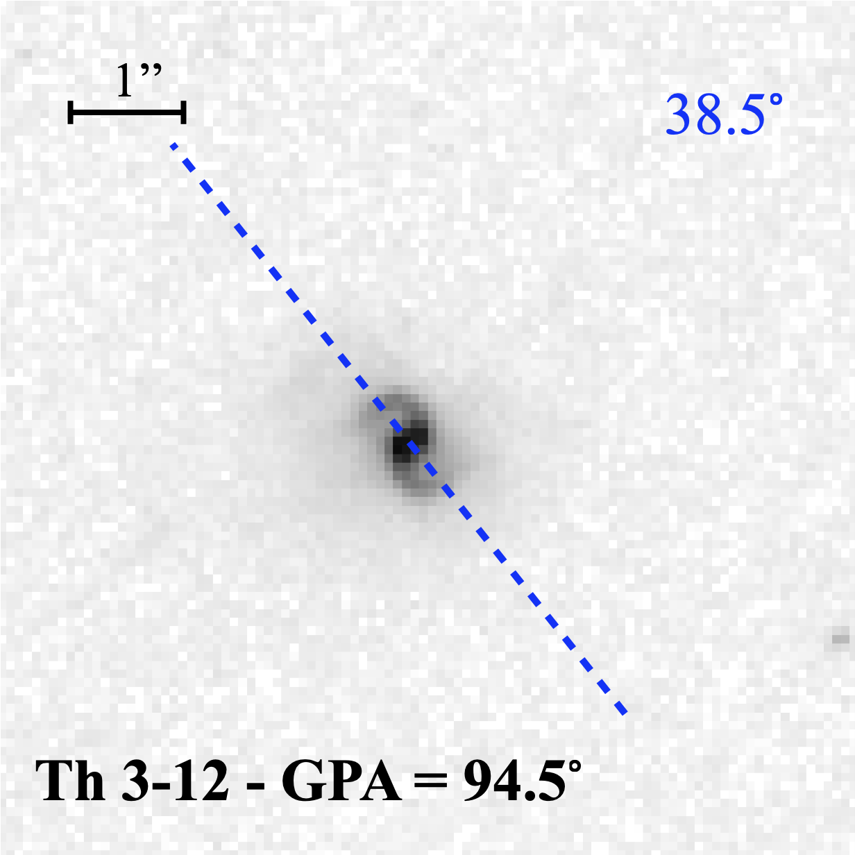
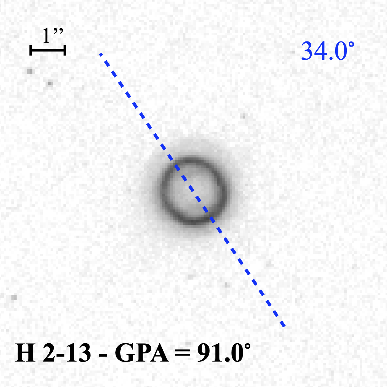
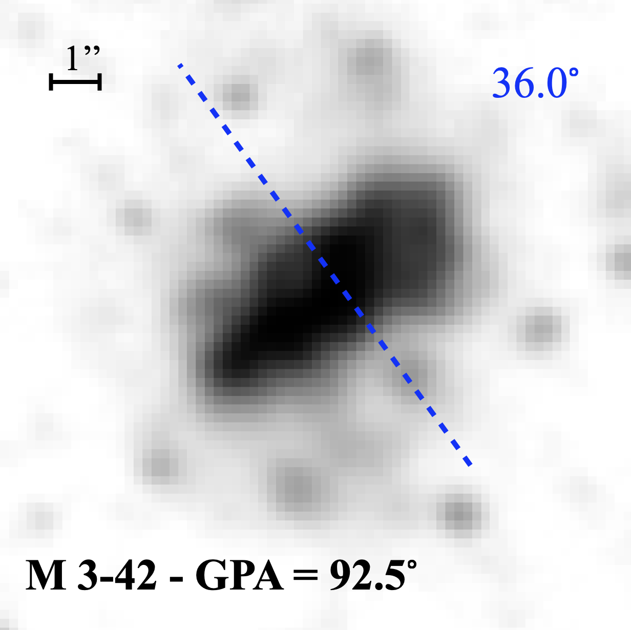
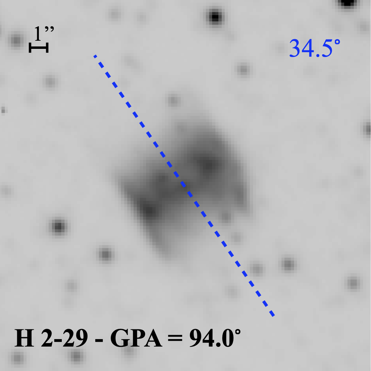
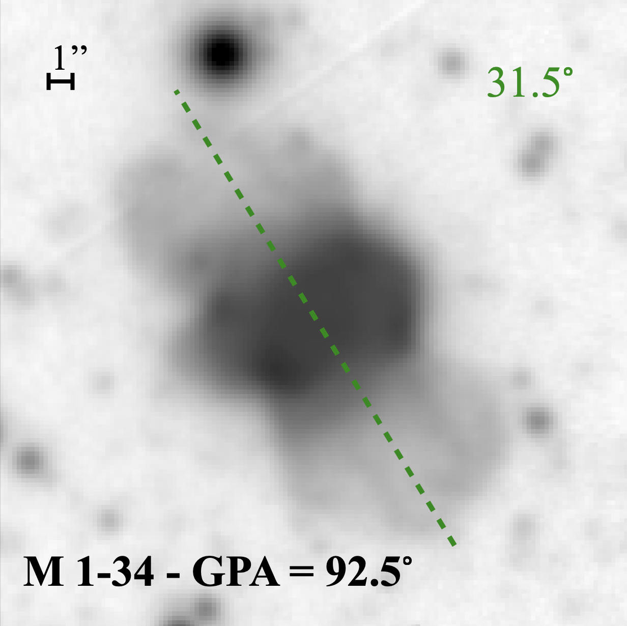
For our Galactic bulge sample of 136 PNe only 6 are in known binary systems and they are all short period binaries: H 2-13, H 2-29, M 2-19, M 3-42, Te 1567 and Th 3-12. One, M 1-34, is suspected of hosting a short period binary but doubts on correct CSPN identification remain. Hence, it is excluded from our analysis but its GPA is consistent with our key finding (see later). All except one, H 2-13, are bipolar, where bipolars constitute of the full bulge sample (see Paper I).
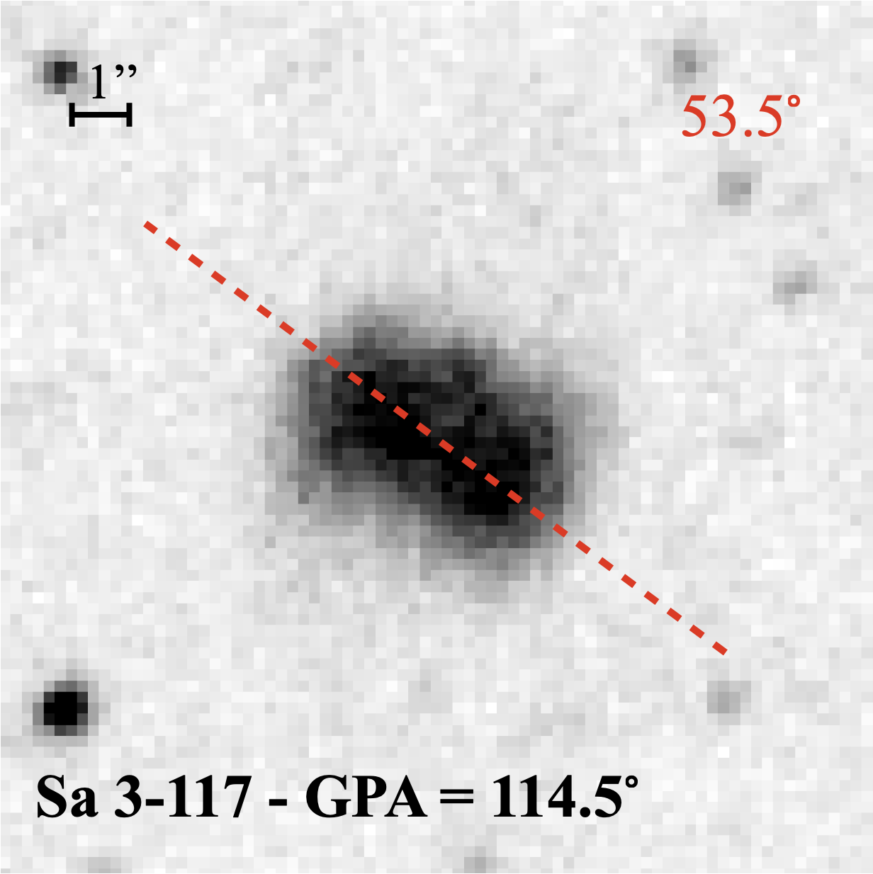
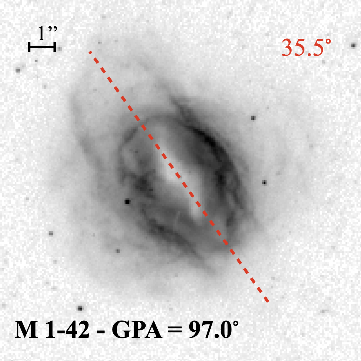
Furthermore, high abundance discrepancy factors (adfs) 18 have been shown by Wesson et al. (2018) to be a reliable proxy for PNe hosting short period binary central stars. An adf is the ratio of elemental abundances obtained from optical recombination lines (ORLs) compared to abundance measurements from collisionally excited lines (CELs), e.g. Corradi et al. (2015); Jones & Boffin (2017); Wesson et al. (2018). We carefully measured adfs for all PNe with sufficient spectral S/N and measurable lines from our VLT spectroscopy. Their derivation and analysis are given Paper IV, Tan et al. (in prep.). We found adfs 18 for 9 PNe in our sample. Of these 8 are bipolars and the other, H 2-42, is a round, annular PN (possibly a pole-on bipolar) that does not yield a GPA. We therefore add this sample to the known short-period binary PNe to provide a total sample of 14 with measurable GPA’s for separate study compared to the full bulge PNe sample and the overall bipolars. The GPAs for PNe with known and inferred short-period binaries are presented in Table 1.
| (a) | |||||||||
| \multirow2*PN G | \multirow2*Name | Period | GPA | \multirow2*Morph. | \multirow2*RAJ2000 | \multirow2*DECJ2000 | D | ||
| [days] | [∘] | [kpc] | [pc] | [kyr] | |||||
| 000.201.9 | M 2-19 | 0.6701 | 165.0 | Brs | 17:53:45.64 | -29:43:47.0 | 6.49 | 0.31 | 21.6 |
| 002.8+01.8 | Te 1567 | 0.1711 | 108.0 | Bars | 17:45:28.34 | -25:38:11.9 | 0.18 | 6.2 | |
| 356.8+03.3 | Th 3-12 | 0.2641 | 94.5 | Bp | 17:25:06.12 | -29:45:17.0 | 0.07 | 5.4 | |
| 357.2+02.0 | H 2-13 | 0.8971 | 91.0 | Emrs | 17:31:08.11 | -30:10:28.2 | 0.09 | 7.8 | |
| 357.5+03.2 | M 3-42 | 0.3201 | 92.5 | Bas | 17:26:59.85 | -29:15:32.7 | 0.20 | 5.10.7 | |
| 357.603.3 | H 2-29 | 0.2442 | 94.0 | Bs | 17:53:16.82 | -32:40:38.5 | 5.37 | 0.16 | 7.4 |
| 357.905.1 | M 1-34∙ | 92.5 | Bmps | 18:01:22.20 | -33:17:43.1 | 0.51 | 17.8 | ||
| (b) | |||||||||
| \multirow2*PN G | \multirow2*Name | \multirow2*adf | GPA | \multirow2*Morph. | \multirow2*RAJ2000 | \multirow2*DECJ2000 | D | ||
| [∘] | [kpc] | [pc] | [kyr] | ||||||
| 000.204.6 | Sa 3-117 | 19.0 | 114.5 | Bs | 18:04:44.09 | -31:02:48.9 | 0.15 | 5.2 | |
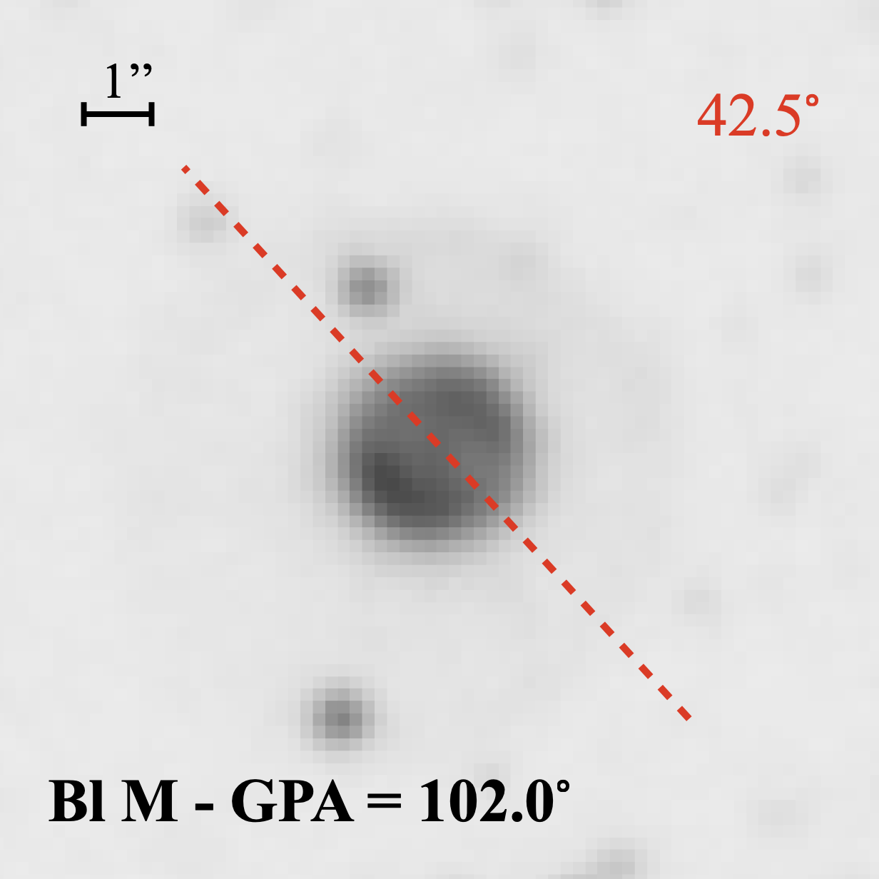
| 001.301.2 | Bl M | 178.4 | 102.0 | Bmrs | 17:53:47.16 | -28:27:17.8 | 4.84 | 0.07 | 2.4 |
| 002.704.8 | M 1-42 | 18.5 | 97.0 | Bamprs | 18:11:04.99 | -28:58:59.2 | 4.31 | 0.19 | 6.9 |
| 005.003.9 | H 2-42 | 147.1 | Ramrs | 18:12:22.99 | -26:32:54.5 | 0.25 | 8.7 | ||
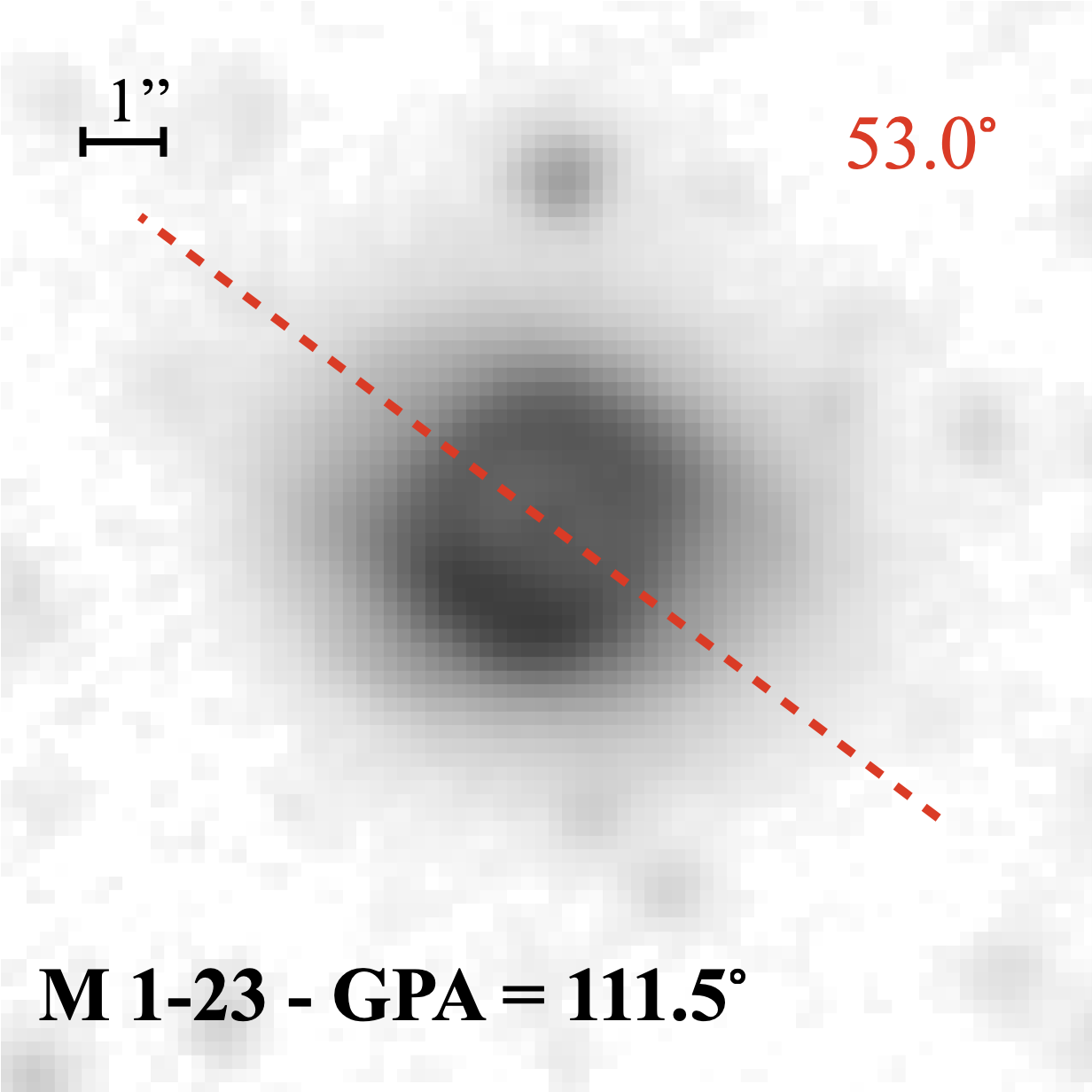
| 007.6+06.9 | M 1-23 | 19.0 | 111.5 | Bamrs | 17:37:22.00 | -18:46:42.0 | 0.32 | 11.1 | |
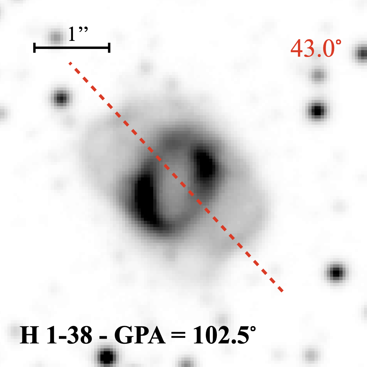
| 353.205.2 | H 1-38 | 42.0 | 102.5 | Bmrs | 17:50:45.20 | -37:23:53.1 | 0.33 | 11.5 | |
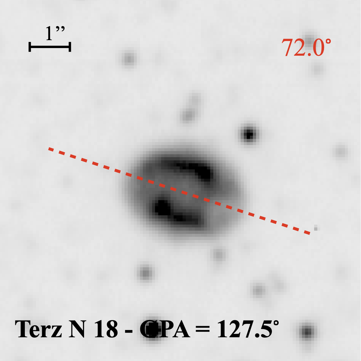
| 357.1+04.4 | Terz N 18 | 19.3 | 127.5 | Ers | 17:21:37.98 | -28:55:14.6 | 0.21 | 7.3 | |
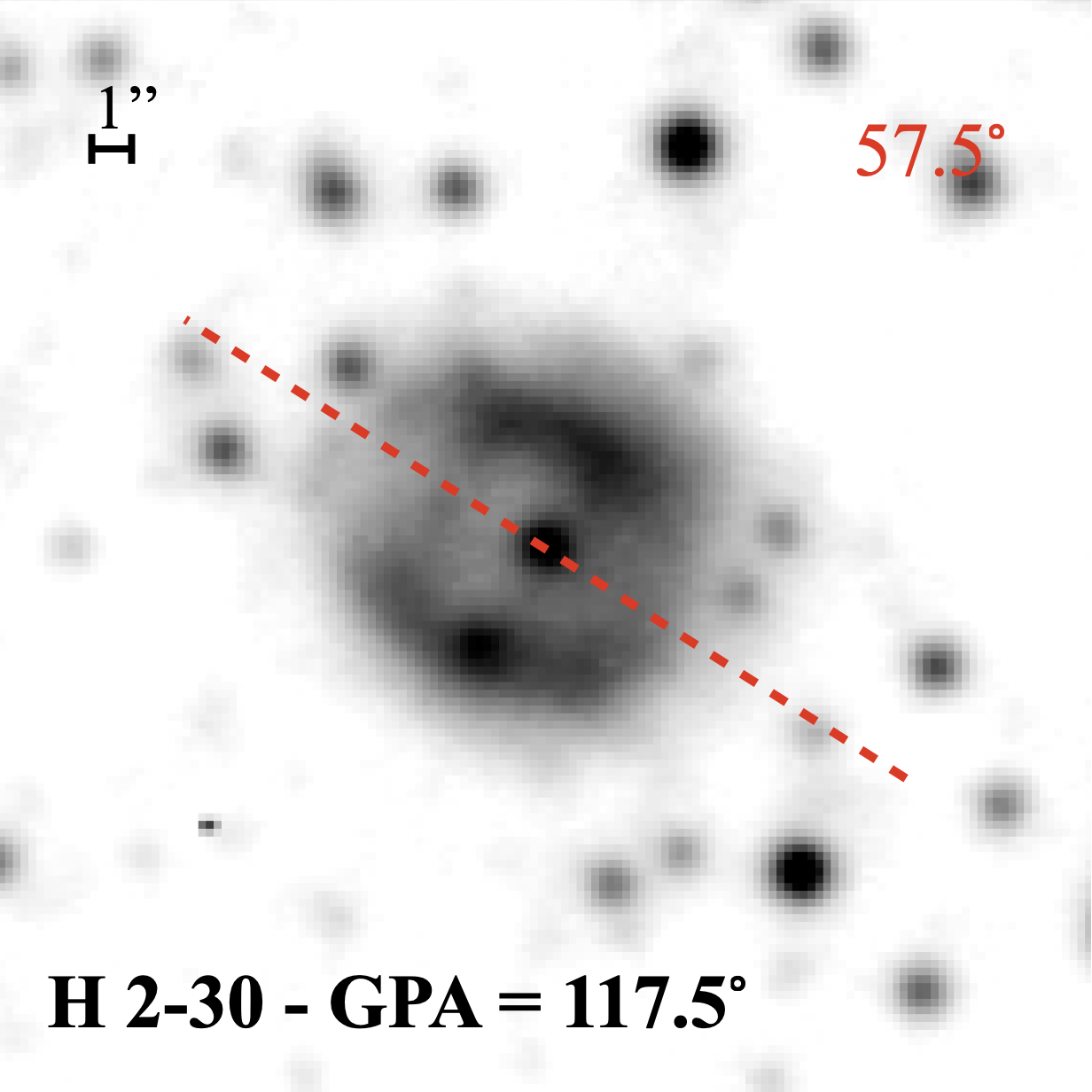
| 357.903.8 | H 2-30 | 184.2 | 117.5 | Bmrs | 17:56:13.93 | -32:37:22.2 | 8.31 | 0.26 | 9.0 |
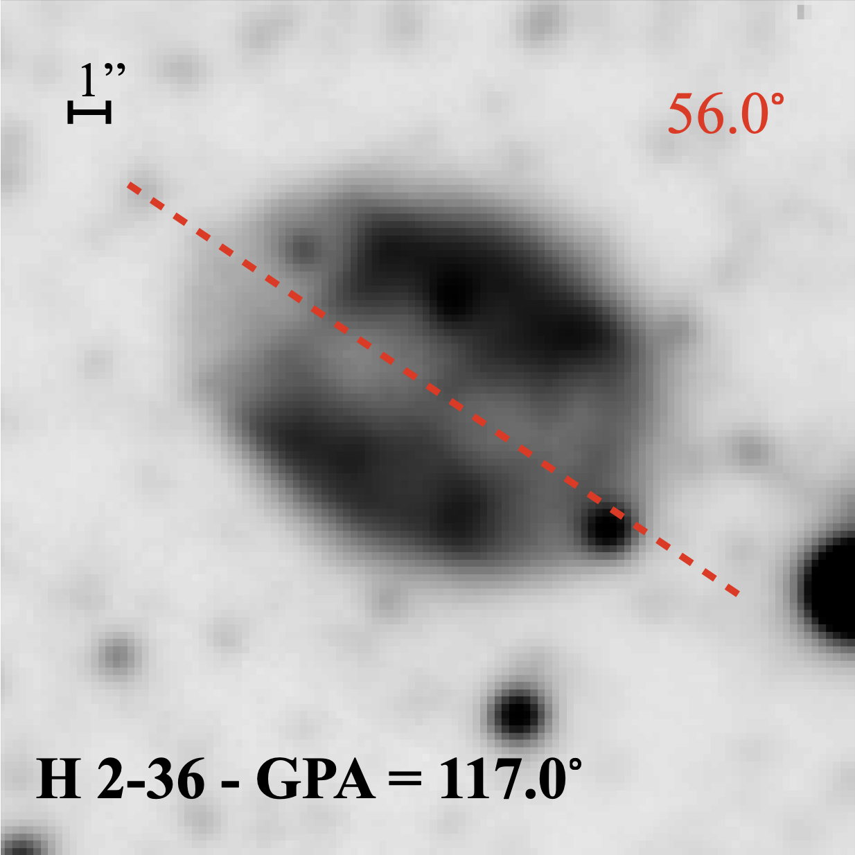
| 359.604.8 | H 2-36 | 51.9 | 117.0 | Brs | 18:04:07.75 | -31:39:10.7 | 0.32 | 11.1 | |
3.2 Measurement of PN position angles
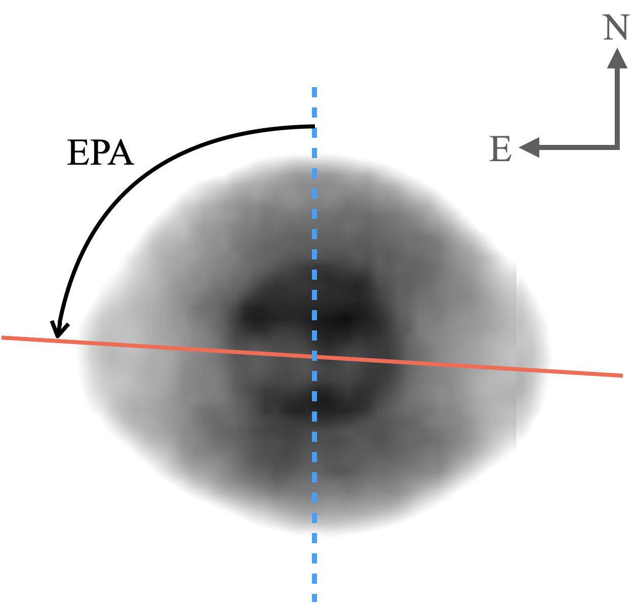
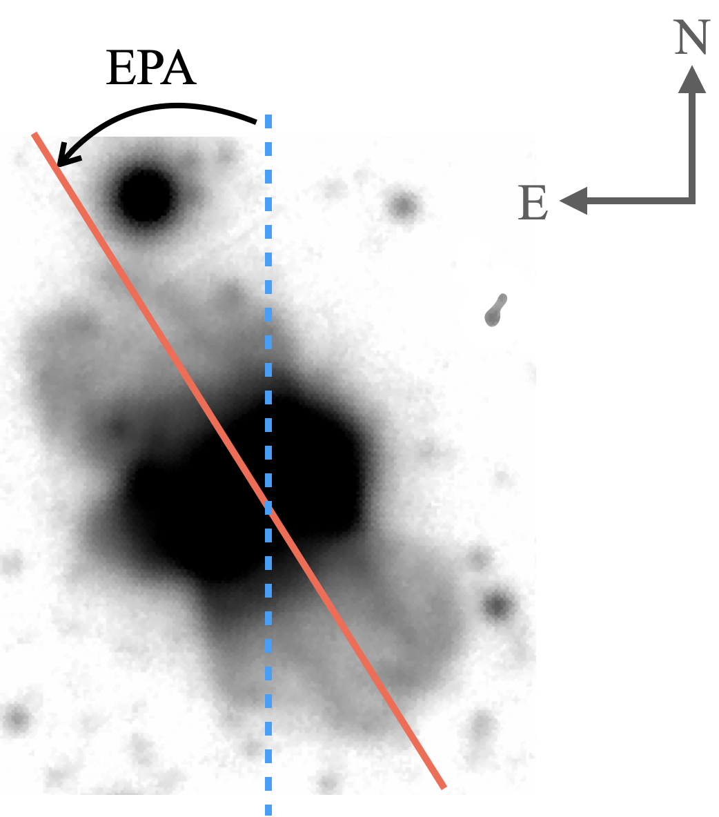
From the combined VLT and HST data of the 136 PNe, a total of 126 could provide a meaningful position angle with the other ten being too round and/or compact. This angle is as measured between the major axis of the apparent nebular elongation from the north towards the east, as shown in Fig. 1. Orientations are measured relative to the PN’s equatorial coordinate system from to , also referred to as the equatorial position angle (EPA). The orientation axis measured from the projected 2-D PN image was determined visually and the axis that best represents the long symmetry of each PN was estimated, taking into account low-density interior structures. EPAs were rounded to the nearest . To determine uncertainties, 50 general Bulge PNe were measured independently by three authors (ST, AR & QAP). This gave a typical difference of - and is considered the random error in our EPA measurements.
The EPAs were converted to Galactic position angles (GPAs) using our measured geometric centroid positions in Galactic coordinates for further analysis. This is following the formula in Corradi et al. (1998) and reproduced below for convenience. This transformation is done by computing the angle subtended at each object’s position by directions of both the equatorial and Galactic north. Using standard relations for spherical triangles, for epoch
where and are the Galactic coordinates of the object. The corrections of for precession of the equinoxes are negligible in the present context. The GPA is then defined as the nebular axis position angle measured from the direction of the Galactic north towards the east,
The uncertainty in GPAs takes the same value as for the EPAs. EPA measurements for the full bulge PNe sample and indeed for confirmed PNe across the rest of the Galaxy (when measurable) will soon be available in Ritter et al. (in prep).
3.3 Statistical Techniques and Analysis
Circular data, as concerned in this study, is a form of directional data in Statistics and a range of texts have been dedicated to describing their special statistical treatment: e.g. Fisher (1995); Mardia et al. (2000); Jammalamadaka & SenGupta (2001); Pewsey et al. (2013), and more recently, Ley & Verdebout (2017); Pewsey (2018). To investigate any GPA alignment signal in our carefully remeasured bulge PNe samples and identify the responsible group, if any, we employed a range of established frequentist tests of circular uniformity on both the entire sample and different subgroups. These subgroups included bipolar PNe, bipolar PNe without confirmed or suspected short-period binaries, all PNe regardless of morphology but excluding the short-period binaries and just the short-period binary PNe. Additionally, we performed Monte Carlo simulations for drawing random samples to test the null hypothesis of uniform distributions by estimating the likelihood of obtaining the observed GPA spread for different subgroups. Further, we used Bayes factors to quantify the evidence in the data in support of a null hypothesis of circular uniformity versus an alternative hypothesis of a von Mises distribution (i.e. circular analogue of the normal distribution, von Mises, 1918). Finally, we used a separate Markov Chain Monte Carlo (MCMC) analysis to fit a von Mises distribution to the observed data when the Bayes factor indicated strong evidence for a von Mises distribution over a uniform distribution.
3.3.1 Frequentist methods
A common statistical exploration of circular data involves testing for the presence of unimodal bias in the distribution around the circle (i.e., a concentration of data in a specific region) or determining if the null hypothesis of a uniform spread throughout the circle is supported by the underlying population. A range of statistical tests have been proposed for this purpose (see Batschelet, 1981, for a review), and applied in previous studies to assess potential biases in the distribution of GPAs in PNe. In our analysis, we used a Rayleigh test, a Kuiper test, a projected Anderson-Darling (PAD) test and a Watson test for a null hypothesis of circular uniformity against an alternative hypothesis of non-uniformity on the doubled GPAs. The statistics were primarily implemented in R (R Core Team, 2021) with unif test of the sphunif package (García-Portugués & Verdebout, 2021) and r.test of the CircStats package (Berens, 2009) for the Rayleigh test. The -values were estimated using the exact null distributions, which were approximated through Monte Carlo simulations. The Rayleigh test is based on the length of the mean vector and is consistent against uni-modal alternatives, e.g. Rayleigh (1919); Fisher (1995); Mardia et al. (2000). The Kuiper and Watson’s tests are based on the maximum and mean differences between empirical and hypothesized uniform cumulative distribution functions (Kuiper, 1960; Batschelet, 1981). They are consistent against all alternatives to uniformity and more sensitive to departures from uniform and multi-modal distributions than the Rayleigh test (Batschelet, 1972). The robustness of the projected Anderson-Darling test used was proven with a simulation study by (García-Portugués et al., 2023) and is a good reference test as it has excellent performance against uni-modal and non uni-modal distributions.
3.3.2 Monte Carlo simulations and Bayesian analysis
To address potential inaccuracies in approximating -values in statistical tests, which may occur with small sample sizes (Ajne, 1968; Freedman, 1981; Arnold & Emerson, 2011), we employed Monte Carlo simulations as an supplementary approach alongside frequentist tests to estimate the likelihood () of obtaining the observed GPAs from a uniform circular distribution. We randomly selected the same number of angles as in the data from a uniform distribution between and times and then calculated the fraction that produced a standard deviation () equal to or smaller than that of the observed data. On this basis, our short-period binary subsample shows an extremely low likelihood of a uniform distribution of GPAs (see results section below).
To further investigate the presence of a concentration of GPAs of our samples, we applied a Bayesian hypothesis test (Mulder & Klugkist, 2021) for circular uniformity against a von Mises alternative based on the Bayes factor, the ratio of two marginal likelihoods, on the doubled GPAs. This was computed using the circbayes package (Mulder, 2021). Flat priors for the mean direction, and the concentration parameter, (1/ is equivalent to the of a normal distribution) were used. The Bayes factors are presented on a log scale in column 7 of Table 2. We follow the standard “rules of thumb” for evidence thresholds outlined in Kass & Raftery (1995). Here, Bayes factors between 20 and 150 () are considered “strong”, while Bayes factors greater than 150 () are labelled as “very strong” evidence for the alternative hypothesis against .
We then applied the MCMC approach to fit a mixture of von Mises distribution to GPAs of the short-period binary sample with emcee (Foreman-Mackey et al., 2013, 2019), an “affine” invariant MCMC implemented in Python (Van Rossum & Drake Jr, 1995). The chosen von Mises distribution has two antipodal modes in 0∘ and 180∘, respectively, to correspond to the practice of our GPA measurement using flat priors where the prior of truncates at 30. We used 500 parallel samplers and 10,000 steps per sampler, with a burn-in period of 6500 steps in all cases. The step size was chosen to adequately sample all parameter spaces based on an analysis of the auto-correlation function of our data as discussed in the emcee documentation333emcee documentation on autocorrelation analysis and convergence can be found at: https://emcee.readthedocs.io/en/latest/tutorials/autocorr.
4 Summary Results
We present statistical analysis results for the five subsets from our bulge PNe sample and summarized in Table 2. The first subset includes all 126 PNe in our sample with a measurable GPA. The second subset consists of 112 PNe that do not host short-period binaries, irrespective of their morphology. The third subset contains all PNe classified as bipolar (93 PNe), while the fourth subset include 81 bipolar PNe but excluding those that also host or are inferred to host short-period binaries. Finally, the fifth subset consists only of 14 PNe hosting short-period binary central stars (i.e. they have measured short-period binary CSPN or have adfs derived from our high S/N, VLT PNe emission line spectroscopy that have been shown are a strong proxy for PNe hosting short period binaries, Wesson et al., 2018).
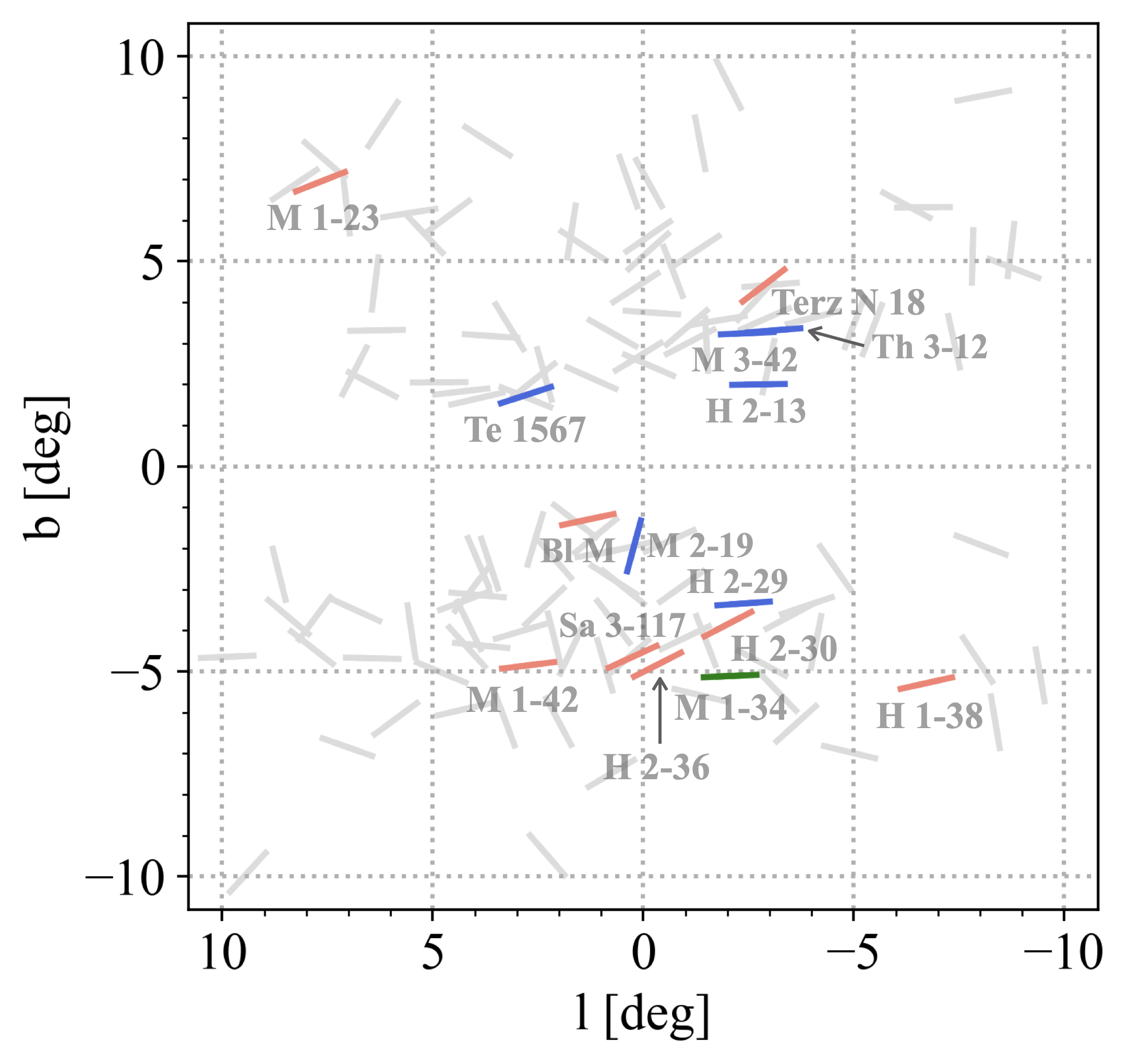
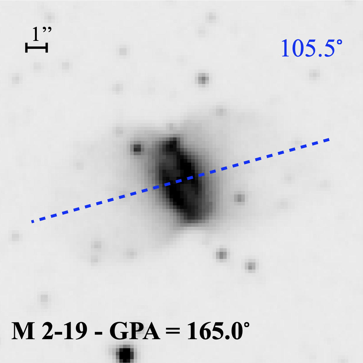
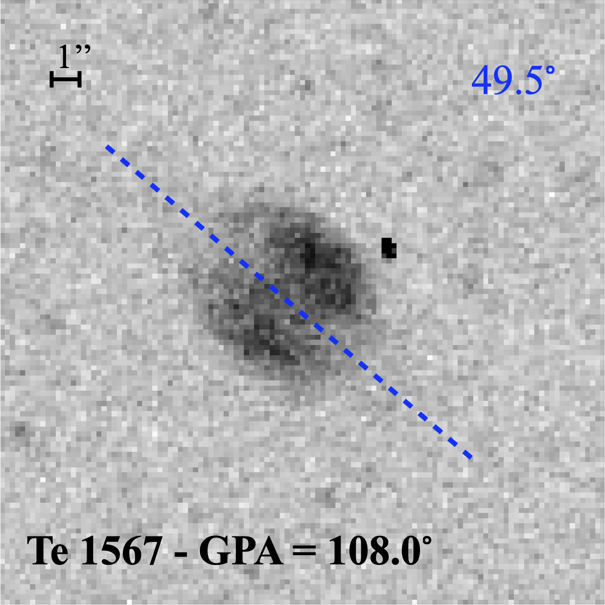
Figure 2 displays the Galactic coordinate distribution for all bulge PNe in our sample with reliable GPA measurements, as well as for the subset of PNe hosting or likely to host short-period binary central stars. The plotted vector orientations indicate the measured GPA, with the six PNe with confirmed short-period binary CSPNe and the eight PNe with high adfs 18 plotted as blue and pink vectors, respectively. The non-binary bulge PN sample is represented by grey vectors. The PN M 1-34, suspected of hosting a short-period binary, is plotted with a green vector. Excluding M 1-34, the combined assumed short-period binary sample has a mean GPA of 107.5∘, with a narrow , indicating a direction nearly parallel to the Galactic plane. In contrast, the non-binary sample has a mean GPA of , with a large for n = 112. Images of all these short-period binary PNe overlaid with the measured GPA vectors are provided in Appendix A.
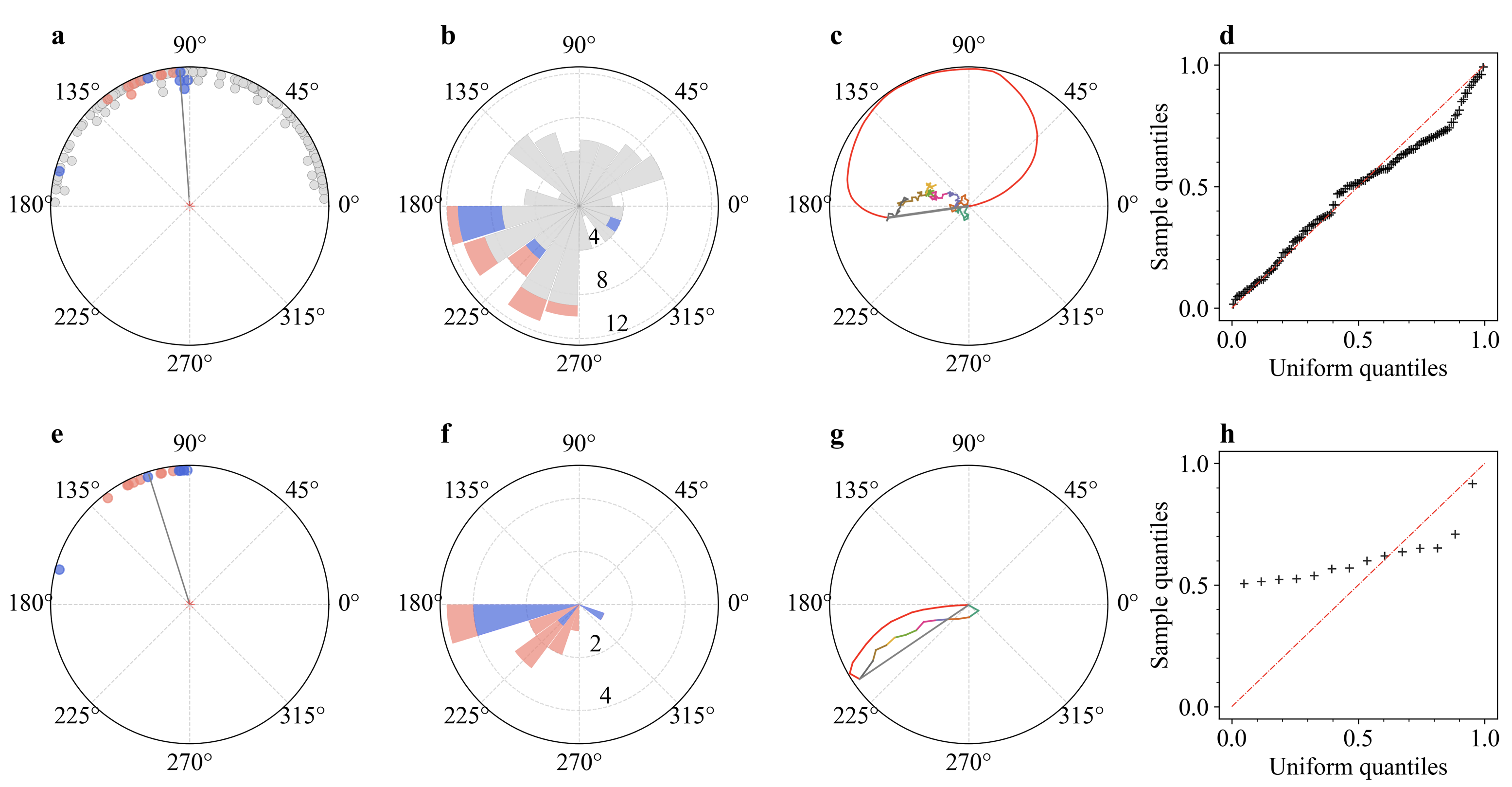
In Fig. 3, we contrast graphical representations for the 126 full PNe sample and the 14 PNe binary sub-sample for which GPA measures were possible. These include finger plots of GPA distribution, rose plots (a circular form of bar chart) of the doubled angles and the quantile–quantile (Q–Q) plots showing deviation from uniformity. The strong, non-uniformity of the GPA’s of the short-period binary sample is obvious. We conducted a Monte Carlo simulation (see Methods) where the estimated likelihood to obtain a 17.5∘ as observed is only 0.0005%. We also applied a Rayleigh test, a Kuiper test, a projected Anderson-Darling test and a Watson test for a null hypothesis of GPA circular uniformity (refer to Methods). The -values, or probabilities that the null hypothesis is true, are listed in columns 2-5 in Table 2 for all four statistical tests.
The results also clearly indicate that the general PNe samples of non short-period binary PNe (regardless of morphology) are highly likely to be uniformly distributed. Furthermore, the bipolar sample of 81 PNe that excludes the short period binary sub-sample show no significant departures from random GPAs.
Our specific short-period binary sample however has a highly significant Rayleigh test statistic and its rose plot in Fig. 3(f) show no multi-modal features that could lead to a type II error (i.e. failure of rejection of the null hypothesis when it is actually false). The Rayleigh test result is reliable, showing a high concentration around a preferred angle direction. The results reported for the the Kuiper and Watson’s tests are also extremely significant in terms of departures from normality for the short-period binary sample which are also almost exclusively bipolar. The weak alignment signal previously reported in Weidmann & Díaz (2008) and even the stronger alignment significance reported by Rees & Zijlstra (2013) for their bipolar sample were both diluted. The actual signal in our study arises solely from a very specific but relatively small PNe sub-sample of short period binary PNe. This is our major discovery.
We also applied a Bayesian hypothesis test using non-informative flat priors (see Methods) to each sample. The Bayes factors for the general bulge PNe sample and the other samples (but excluding the short-period binary sub-sample) provide positive evidence for the alternative hypothesis of a von Mises unimodal circular distribution. For our full bipolar subsample the Bayes factor does give some weak support for a von Mises distribution c.f. a uniform distribution with . However, the Bayes factor for the short-period binary subsample is a remarkable and provides extremely strong preference for a concentrated von Mises distribution.
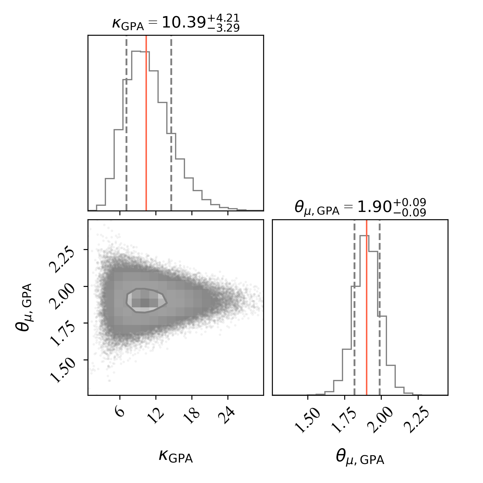
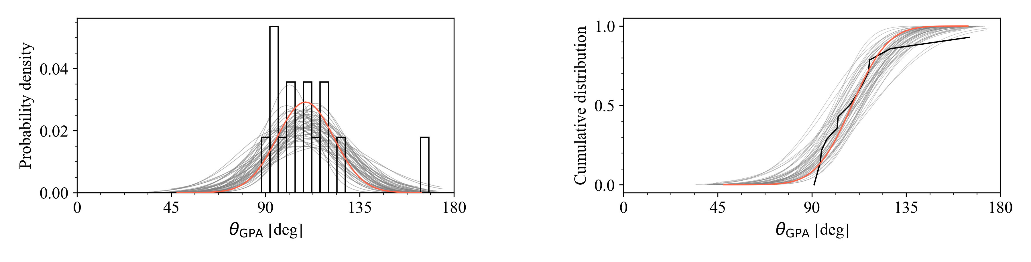
Through an MCMC analysis, we find the most likely values for the orientation and standard deviation of the binary sub-sample are and degrees, respectively. The presented lower and upper errors correspond to the and percentiles of the samples, which coincides with 1 confidence levels in the case of a Gaussian posterior distribution. The associated “corner plot” is presented in Fig. B1 of Appendix B, displaying the results of MCMC parameter estimation of the von Mises model applied to our short-period binary PN sample. Additionally, we provide a comparison between the model estimations and the observed data in Fig. B2. The alignment of GPAs of our short-period binary subsample is further supported by the observed high concentration parameter .
Hence, regardless of the statistical approach applied, the GPAs of our short-period binary PNe sub-sample are highly concentrated. This is the first time preferred PNe major axes alignments have been demonstrated with such high statistical power but only for a special sub-sample of PNe that host, or are inferred to host, short-period binary CSPN. These are almost exclusively bipolars () and so are likely also to be undergoing common envelope evolution (CEE), e.g. Ivanova et al. (2013). What could be the explanation?
One key consideration is at what evolutionary stage is the effect imposed? If the effect reflects today a respect for a binary orbit inclination “frozen in” at the time of the original binary system formation then an enduring longevity of the causality must exist. This is because such systems did not all form at the same time but over hundreds of millions of years and perhaps billions of years ago. If the effect is imposed very recently on all these short lived PNe visible now, and in just those systems where the binary orbits have decayed to short periods and on entering a CEE phase, then what fast acting mechanism can do this?
| Sample | B | |||||
|---|---|---|---|---|---|---|
| All (126) | 0.024 [2.3] | 0.0062 [2.7] | 0.13 [1.5] | 0.013 [2.5] | 0.024 [2.3] | 1.1 |
| Non-SP Binary (112) | 0.26 [1.1] | 0.13 [1.5] | 0.99 [0.0] | 0.22 [1.2] | 0.26 [1.1] | 0.26 |
| B (93) | 0.023 [2.3] | 0.022 [2.3] | 0.085 [1.7] | 0.014 [2.5] | 0.022 [2.3] | 1.2 |
| B, Non-SP Binary (81) | 0.17 [1.4] | 0.17 [1.4] | 0.84 [0.2] | 0.18 [1.3] | 0.17 [1.4] | 0.57 |
| SP Binaries (14) | 5.0 [4.6] | 1.2 [4.9] | 2.8 [4.7] | 2.9 [4.7] | 5.0 [4.6] | 5.5 |
5 Discussion and Speculation
The bulge PNe currently going through the short-lived PNe phase, regardless of whether in a binary or even triple system with other companions (including planets), could have a range of progenitor masses, as suggested by Bensby et al. (2013, 2017). The progenitors will not have been born at the same time. Gesicki et al. (2014) derive an extended star formation history from bulge PNe. For example, a range of 1 solar mass at stellar birth would mean a difference of hundreds of millions of years for stars born with masses between 2 and 3 M⊙ (see Fig. 3 in Buzzoni, 2002) based on evolutionary models of single stars. In a PNe hosting a binary or even multiple system, only one of the stars is currently going through the PNe phase as it reaches that particular stage of evolution.
By chance, two such PNe in our short-period binary sub-sample have had their CSPN ages previously estimated by Gesicki et al. (2014), namely Th 3-12 (PNG 356.8+03.3) and H 2-13 (PNG 357.2+02.2), at 7 and 10 Gigayears respectively (but based on a single-star model). Hence, if the observed GPAs of their major bipolar lobes do indeed reflect the inclinations of their binary orbits today, and if these orbital inclinations originate from system birth, then the causal influence acting on star formation has to have endured, effectively unchanged, for cosmologically significant time periods. The difference of about 3 Gigayears just for the two examples above suggests that the alignment process was not caused in a single star formation burst but acted for at least several Gyr.
Why do only the bipolars with short-period binaries demonstrate the astonishing GPA alignment shown across several kpc of the Galactic bulge? A possible explanation that other bipolars are not in (close) binary systems is contrary to currently accepted wisdom for how bipolars form e.g. Ondratschek et al. (2022). Our results imply that more than one type of systems forms bipolar nebulae, given only a modest fraction of observed bipolars fit the bill. Perhaps the observed alignment effect is also a function of the separation of the binary components at system birth? Note that close binary CSPN have isolated binary evolution and the angular momentum vector of the system remains constant after formation. The only other alternative is a physical process operating now in the Galactic bulge but only on bipolar PNe in short period binaries, that aligns their bipolar ejecta over the short timescales that these PNe are now visible (only a few tens of thousands of years).
PNe axes of symmetry are thought to trace the rotation of their CSPN which may themselves align with a very strong interstellar magnetic field at their time of formation from the collapsing disks of rotating molecular gas where the orbital inclinations, if also part of a binary or multiple system, are established (Rees & Zijlstra, 2013). An alternative is they may possibly be directly tilted later by the extant magnetic field itself (Falceta-Gonçalves & Monteiro, 2014). Binary star systems may have formed long ago in the presence of a strong Galactic magnetic field where their orbits align with this field due to their higher angular momenta compared with single-star systems (Rees & Zijlstra, 2013). Indeed, it is reported by Price & Bate (2007) that magnetic fields have important effects on molecular cloud core fragments and on their subsequent condensation and formation of binary systems. They report the scale of binary separation at birth as an important factor in the level of binary orbit to magnetic field alignment eventually achieved with the effect more pronounced at shorter separations.
Symmetry axes of PNe ejecta from one of the stars within binary systems take the axes of their angular momenta. The magnetic field in the Galactic bulge was proposed to counter the contraction of any star-forming cloud perpendicular to the direction of the Galactic plane during the early phases of bulge star formation (e.g. Price & Bate, 2007; Gray et al., 2018). However, we observe the preferential major axis orientation only in objects with confirmed or inferred short-period binaries that have also likely undergone a CEE phase. These objects may have been in tighter orbits to begin with before then spiralling in for the CEE phase and may have higher angular momentum. PNe that avoid a CEE would have much wider orbits at birth.
According to Falceta-Gonçalves & Monteiro (2014) PNe symmetry axes modification can occur if the local magnetic field is . From optical polarization measures, radio synchrotron data and Zeeman splitting seen in object spectra, the average total magnetic field strength in the bulge today is 20-40 G (LaRosa et al., 2005). This is likely insufficient to modify binary orbital inclinations over the short timescales implied before the bulge PNe we see today are formed. It is more plausible the observed effect was “frozen in” in the past. The simulations of Falceta-Gonçalves & Monteiro (2014) show further orbit modification can occur at t 104 years after PN envelope ejection, compared with the rapid CEE timescaled expected (a few years or even less, Ivanova et al., 2013). This might not happen to post-CEE PNe that form our short period binary sample. Only post-CEE PNe may maintain their ancient orientations resulting from their orbital angular momenta aligning with the initial (presumably historically stronger) magnetic field at their formation time along the Galactic plane. This assumes they originally had tighter orbits following the arguments of Price & Bate (2007).
PNe formed from wider binaries could have their symmetry axes change over time more randomly due to the ambient field where directions may evolve due to a Galactic wind or bulk motions of the ISM. This provides a possible explanation for the observed effect only being seen in post-CE binary PNe. If this is the process then it must remain ordered, stay potent and have endured for billions of years. The only alternative is a pervasive force (magnetic?) acting currently only on the bipolar lobe ejection mechanism in PNe hosting short period binaries that is sufficiently strong to align GPA’s over the entire Galactic bulge in a few thousand years.
Acknowledgements
We are grateful to the referee and statistics editor whose comments and suggestions have significantly improved the paper. S.T. thanks HKU and Q.A.P. for provision of an MPhil scholarship and subsequent Research Assistant position, Q.A.P. thanks the Hong Kong Research Grants Council for GRF research support under grants 17326116 and 17300417. A.R. thanks HKU for the provision of postdoctoral fellowship under Q.A.P. A.A.Z. thanks the Hung Hing Ying Foundation for a visiting HKU professorship and acknowledges UK STFC funding under grant ST/T000414/1. This work made use of the University of Hong Kong/Australian Astronomical Observatory/Strasbourg Observatory H-alpha Planetary Nebula (HASH PN) database, hosted by the Laboratory for Space Research at the University of Hong Kong. We acknowledge use of ESO observations under program IDs 095.D-0270(A), 097.D-0024(A), 099.D-0163(A), and 0101.D-0192(A) for PI Rees. We acknowledge use of data from the Wide Field and Planetary Camera 2 Instrument (WFPC2) of the HST through HST-SNAP-8345 (PI: Sahai), HST-SNAP-9356 (PI: Zijlstra) and HST-GO-11185 (PI: Rubin). Some data presented in this paper were obtained from the Mikulski Archive for Space Telescopes (MAST) at the Space Telescope Science Institute. The specific observations analyzed can be accessed viahttps://doi.org/10.17909/pej3-ce46 (catalog doi:0.17909/pej3-ce46).
References
- Ajne (1968) Ajne, B. 1968, Biometrika, 55, 343
- Aller et al. (2020) Aller, A., Lillo-Box, J., Jones, D., Miranda, L. F., & Forteza, S. B. 2020, Astronomy & Astrophysics, 635, A128
- Appenzeller et al. (1998) Appenzeller, I., Fricke, K., Fürtig, W., et al. 1998, The messenger, 94
- Arnold & Emerson (2011) Arnold, T. B., & Emerson, J. W. 2011, R Journal, 3
- Astropy Collaboration et al. (2018) Astropy Collaboration, Price-Whelan, A. M., Sipőcz, B. M., et al. 2018, AJ, 156, 123
- Batschelet (1972) Batschelet, E. 1972, NASA, Washington Animal Orientation and Navigation
- Batschelet (1981) —. 1981, ACADEMIC PRESS, 111 FIFTH AVE., NEW YORK, NY 10003, 1981, 388
- Bensby et al. (2013) Bensby, T., Yee, J., Feltzing, S., et al. 2013, Astronomy & Astrophysics, 549, A147
- Bensby et al. (2017) Bensby, T., Feltzing, S., Gould, A., et al. 2017, Astronomy & Astrophysics, 605, A89
- Berens (2009) Berens, P. 2009, Journal of statistical software, 31, 1
- Blitz et al. (1993) Blitz, L., Binney, J., Lo, K., Bally, J., & Ho, P. T. 1993, Nature, 361, 417
- Boffin & Jones (2019) Boffin, H. M., & Jones, D. 2019, The Importance of Binaries in the Formation and Evolution of Planetary Nebulae (Springer)
- Buzzoni (2002) Buzzoni, A. 2002, AJ, 123, 1188
- Chornay et al. (2021) Chornay, N., Walton, N., Jones, D., et al. 2021, Astronomy & Astrophysics, 648, A95
- Corradi et al. (1998) Corradi, R. L., Aznar, R., & Mampaso, A. 1998, Monthly Notices of the Royal Astronomical Society, 297, 617
- Corradi et al. (2015) Corradi, R. L., García-Rojas, J., Jones, D., & Rodríguez-Gil, P. 2015, The Astrophysical Journal, 803, 99
- Crutcher (2012) Crutcher, R. M. 2012, Annual Review of Astronomy and Astrophysics, 50, 29
- Danehkar & Parker (2016) Danehkar, A., & Parker, Q. A. 2016, in Star Clusters and Black Holes in Galaxies across Cosmic Time, ed. Y. Meiron, S. Li, F. K. Liu, & R. Spurzem, Vol. 312, 128–130
- De Marco (2009) De Marco, O. 2009, Publications of the Astronomical Society of the Pacific, 121, 316
- Falceta-Gonçalves & Monteiro (2014) Falceta-Gonçalves, D., & Monteiro, H. 2014, Monthly Notices of the Royal Astronomical Society, 438, 2853
- Fisher (1995) Fisher, N. I. 1995, Statistical analysis of circular data (cambridge university press)
- Foreman-Mackey et al. (2013) Foreman-Mackey, D., Hogg, D. W., Lang, D., & Goodman, J. 2013, Publications of the Astronomical Society of the Pacific, 125, 306
- Foreman-Mackey et al. (2016) Foreman-Mackey, D., et al. 2016, J. Open Source Softw., 1, 24
- Foreman-Mackey et al. (2019) Foreman-Mackey, D., Farr, W., Sinha, M., et al. 2019, Journal of Open Source Software
- Freedman (1981) Freedman, L. 1981, Biometrika, 68, 708
- García-Portugués et al. (2023) García-Portugués, E., Navarro-Esteban, P., & Cuesta-Albertos, J. A. 2023, Bernoulli, 29, 181
- García-Portugués & Verdebout (2021) García-Portugués, E., & Verdebout, T. 2021, sphunif: Uniformity Tests on the Circle, Sphere, and Hypersphere, r package version 1.0.1. https://CRAN.R-project.org/package=sphunif
- Gesicki et al. (2014) Gesicki, K., Zijlstra, A., Hajduk, M., & Szyszka, C. 2014, Astronomy & Astrophysics, 566, A48
- Gesicki et al. (2014) Gesicki, K., Zijlstra, A. A., Hajduk, M., & Szyszka, C. 2014, A&A, 566, A48
- González-Santamaría et al. (2020) González-Santamaría, I., Manteiga, M., Manchado, A., et al. 2020, Astronomy & Astrophysics, 644, A173
- Gray et al. (2018) Gray, W. J., McKee, C. F., & Klein, R. I. 2018, Monthly Notices of the Royal Astronomical Society, 473, 2124
- Grinin & Zvereva (1968) Grinin, V. P., & Zvereva, A. M. 1968, Astrophysics, 4, 43
- Han et al. (1995) Han, Z., Podsiadlowski, P., & Eggleton, P. P. 1995, Monthly Notices of the Royal Astronomical Society, 272, 800
- Hunter (2007) Hunter, J. D. 2007, Computing in science & engineering, 9, 90
- Ivanova et al. (2013) Ivanova, N., Justham, S., Chen, X., et al. 2013, The Astronomy and Astrophysics Review, 21, 1
- Jacoby et al. (2021) Jacoby, G. H., Hillwig, T. C., Jones, D., et al. 2021, Monthly Notices of the Royal Astronomical Society, 506, 5223
- Jammalamadaka & SenGupta (2001) Jammalamadaka, S. R., & SenGupta, A. 2001, Topics in circular statistics, Vol. 5 (world scientific)
- Jones & Boffin (2017) Jones, D., & Boffin, H. M. 2017, Nature Astronomy, 1, 117
- Kass & Raftery (1995) Kass, R. E., & Raftery, A. E. 1995, Journal of the american statistical association, 90, 773
- Kormendy & Kennicutt Jr (2004) Kormendy, J., & Kennicutt Jr, R. C. 2004, Annu. Rev. Astron. Astrophys., 42, 603
- Kuiper (1960) Kuiper, N. H. 1960, in Indagationes Mathematicae (Proceedings), Vol. 63, Elsevier, 38–47
- Kwitter & Henry (2022) Kwitter, K. B., & Henry, R. 2022, Publications of the Astronomical Society of the Pacific, 134, 022001
- LaRosa et al. (2005) LaRosa, T. N., Brogan, C. L., Shore, S. N., et al. 2005, The Astrophysical Journal, 626, L23
- Ley & Verdebout (2017) Ley, C., & Verdebout, T. 2017, Modern directional statistics (CRC Press)
- Mardia et al. (2000) Mardia, K. V., Jupp, P. E., & Mardia, K. 2000, Directional statistics, Vol. 2 (Wiley Online Library)
- McKee & Ostriker (2007) McKee, C. F., & Ostriker, E. C. 2007, Annu. Rev. Astron. Astrophys., 45, 565
- Miszalski et al. (2009) Miszalski, B., Acker, A., Moffat, A. F., Parker, Q. A., & Udalski, A. 2009, Astronomy & Astrophysics, 496, 813
- Morris (1981) Morris, M. 1981, Astrophysical Journal, Part 1, vol. 249, Oct. 15, 1981, p. 572-585., 249, 572
- Morris (1987) —. 1987, Publications of the Astronomical Society of the Pacific, 99, 1115
- Mulder (2021) Mulder, K. T. 2021, circbayes: Bayesian analysis of circular data., r package version 0.1.0.9000. https://github.com/keesmulder/circbayes
- Mulder & Klugkist (2021) Mulder, K. T., & Klugkist, I. 2021, Journal of Statistical Planning and Inference, 211, 315
- Ondratschek et al. (2022) Ondratschek, P. A., Röpke, F. K., Schneider, F. R., et al. 2022, Astronomy & Astrophysics, 660, L8
- Ondratschek et al. (2022) Ondratschek, P. A., Röpke, F. K., Schneider, F. R. N., et al. 2022, A&A, 660, L8
- Parker (2022) Parker, Q. A. 2022, Frontiers in Astronomy and Space Sciences, 9, 895287
- Parker et al. (2016) Parker, Q. A., Bojičić, I. S., & Frew, D. J. 2016, in Journal of Physics: Conference Series, Vol. 728, IOP Publishing, 032008
- Parker et al. (2006) Parker, Q. A., Acker, A., Frew, D. J., et al. 2006, Monthly Notices of the Royal Astronomical Society, 373, 79
- Pewsey (2018) Pewsey, A. 2018, Applied Directional Statistics, 293
- Pewsey et al. (2013) Pewsey, A., Neuhäuser, M., & Ruxton, G. D. 2013, Circular statistics in R (Oxford University Press)
- Price & Bate (2007) Price, D. J., & Bate, M. R. 2007, Monthly Notices of the Royal Astronomical Society, 377, 77
- R Core Team (2021) R Core Team. 2021, R: A Language and Environment for Statistical Computing, R Foundation for Statistical Computing, Vienna, Austria. https://www.R-project.org/
- Rayleigh (1919) Rayleigh, L. 1919, The London, Edinburgh, and Dublin Philosophical Magazine and Journal of Science, 37, 321
- Rees & Zijlstra (2013) Rees, B., & Zijlstra, A. 2013, Monthly Notices of the Royal Astronomical Society, 435, 975
- Robitaille (2019) Robitaille, T. 2019, Zenodo
- Robitaille & Bressert (2012) Robitaille, T., & Bressert, E. 2012, Astrophysics Source Code Library, ascl
- Soker (1998) Soker, N. 1998, ApJ, 496, 833
- Soker & Livio (1994) Soker, N., & Livio, M. 1994, The Astrophysical Journal, 421, 219
- Tan et al. (2023) Tan, S., Parker, Q. A., Zijlstra, A., & Ritter, A. 2023, Monthly Notices of the Royal Astronomical Society, 519, 1049
- Van Der Walt et al. (2011) Van Der Walt, S., Colbert, S. C., & Varoquaux, G. 2011, Computing in science & engineering, 13, 22
- Van Rossum & Drake Jr (1995) Van Rossum, G., & Drake Jr, F. L. 1995, Python reference manual (Centrum voor Wiskunde en Informatica Amsterdam)
- Virtanen et al. (2020) Virtanen, P., Gommers, R., Oliphant, T. E., et al. 2020, Nature Methods, 17, 261
- von Mises (1918) von Mises, R. 1918, Physikalische Zeitschrift, 19, 490
- Weidmann & Díaz (2008) Weidmann, W. A., & Díaz, R. J. 2008, Publications of the Astronomical Society of the Pacific, 120, 380
- Wesson et al. (2018) Wesson, R., Jones, D., García-Rojas, J., Boffin, H., & Corradi, R. 2018, Monthly Notices of the Royal Astronomical Society, 480, 4589
Appendix A: PN Images and GPAs
| (a) |
| (b) |
Appendix B: Posterior distributions of von Mises parameters obtained by applying emcee on our short-period binary PN sample.