When Standard Model Higgs Meets Its Lighter 95 GeV Higgs
Abstract
Two excesses reported recently at the LHC in the lighter Higgs mass region around 95 GeV and in the rare final state of the Standard Model (SM) 125 GeV Higgs decay are simultaneously scrutinized within the framework of minimal gauged two-Higgs-doublet model (G2HDM). Viable parameter space in G2HDM is obtained to account for both excesses. We find a strong correlation between the signal strengths of SM 125 GeV Higgs decays into and modes, whereas this correlation does not extend to its lighter 95 GeV cousin.
I Introduction
Facing the mounting several hundreds petabytes of physics data collected by the Large Hadron Collider (LHC) since the first collision at 2010, Standard Model (SM) is holding up amazingly well, surviving all the challenges posted by our experimental colleagues. Albeit there were reports from the LHC over the years about some middling 23 excesses and created some excitements in the community, the joys did not last long as the excesses faded away quickly when more statistics was accumulated. Nevertheless, few people would doubt there must be new physics beyond the SM (BSM). From the bottom-up viewpoint, right-handed neutrinos are seem to be required as suggested by the experiments of neutrino oscillations. Dark matter and dark energy are also missing in SM but they are essential ingredients for the evolution and history of our observed universe. From the top-down viewpoint, we also have good arguments for new physics from grand unification, gauge hierarchy problem, theory of everything like string theory, etc.
Recently, CMS has reported an excess in the light Higgs-boson search in the di-photon () decay mode at about 95.4 GeV based on the 8 TeV data and the full Run 2 data set at 13 TeV with the local significance is CMS (2023). The corresponding signal strength is given as
| (1) |
where denotes the cross section for a hypothetical scalar boson with the mass is 95.4 GeV, and is the SM Higgs.
ATLAS recently also presented the result of the search for new neutral scalars in the di-photon final state with mass window from 66 GeV to 110 GeV, using full Run 2 data collected at 13 TeV ATLAS ; ATL (2023). ATLAS observed an excess at the same mass value as reported by the CMS with the local significance is . The corresponding signal strength is given as Biekötter et al. (2023a)
| (2) |
The combined local significance from ATLAS and CMS is and the signal strength is Biekötter et al. (2023a)
| (3) |
Using the full Run 2 data set, CMS reported another local excess with a significance of () for light Higgs with mass GeV ( GeV) produces from gluon-gluon fusion and subsequently decays to di-tau () final state CMS (2022). The signal strength for the scalar mass at GeV is given as
| (4) |
Note that ATLAS has not yet reported a search in the di-tau final state that covers the mass range around 95 GeV.
In additional, searches for a low-mass scalar boson were previously carried out at LEP. A local significance excess of for the light scalar mass of about 98 GeV in the process and the corresponding signal strength of Barate et al. (2003)
| (5) |
At face values, the signal strengths in (3), (4) and (5) indicate that the 95 GeV Higgs, if its existence is confirmed, would be very much SM-like for the di-tau mode but rather non-SM like for both the di-photon and modes. Excesses in these channels are strong motivation for BSM. Indeed in light of these excesses, many BSMs have been studied in recent years, e.g. Dev et al. (2023); Li et al. (2023); Chen et al. (2023); Ahriche (2023); Arcadi et al. (2023); Ahriche et al. (2023); Borah et al. (2023); Cao et al. (2023); Ellwanger and Hugonie (2023); Dutta et al. (2023); Aguilar-Saavedra et al. (2023); Ashanujjaman et al. (2023); Belyaev et al. (2023); Escribano et al. (2023); Azevedo et al. (2023); Biekötter et al. (2023b); Iguro et al. (2022); Biekötter et al. (2022); Sachdeva and Sadhukhan (2020); He et al. (2024).
More recently, ATLAS and CMS Collaborations Aad et al. (2024) reported an analysis for the first evidence of the rare decay mode , where the boson decays into a or pair. The number of events is found twice as many as predicted by the SM. To be more precise, the combined observed signal yield is
| (6) |
with a 3.4 statistical significance.
Currently, the data are insufficient to rule out the possibility that the above discrepancies are merely statistical fluke. Nevertheless, they open up the opportunity window for new physics.
Is this paper, we study the excesses (3), (4), (5) and (6) in the framework of minimal gauged two-Higgs-doublet model (G2HDM) which contains a predominantly singlet scalar , a mixture of a hidden scalar with the SM Higgs boson, can become the 95 GeV Higgs boson candidate. The orthogonal combination will be identified as the observed 125 GeV Higgs boson. Besides the SM boson and top quark contributions, the presence of charged heavy hidden fermions and charged Higgs can provide additional contributions to the production and decay through one-loop diagrams for both Higgs bosons. Thus it is natural that the signal strengths for these two Higgs bosons deviate from their SM expectations.
This paper is organized as follows. We will give a brief review of the minimal G2HDM in Section II, followed by a discussion in Section III for the computation of signal strengths in the model. Numerical studies of scanning the parameter space in G2HDM are presented in Section IV. We conclude in Section V. For convenience, Appendix A collects the detailed decay rates for , and modes of the Higgs bosons. We also discuss our numerical study of the two loop functions entered in the Higgs decay amplitudes.
II The Minimal G2HDM
The crucial idea of the original G2HDM Huang et al. (2016a) was to embed the two Higgs doublets and in the popular scalar dark matter model, the inert two-Higgs-doublet model (I2HDM), into a 2-dimensional irreducible representation of a hidden gauge group , a dark replica of the SM electroweak group . Besides the two Higgs doublets in I2HDM, the original G2HDM also introduced two hidden scalar multiplets, one doublet () and one triplet (), to generate the hidden particle mass spectra. The hidden gauge group acts horizontally on the two Higgs doublets in I2HDM.
Various refinements Arhrib et al. (2018); Huang et al. (2019); Chen et al. (2020) and collider phenomenology Huang et al. (2016b); Chen et al. (2019); Huang et al. (2018) were pursued subsequently with the same particle content as in the original model. Recently Ramos et al. (2021a, b), it has been realized that removing the hidden triplet scalar field in the model without jeopardizing a realistic hidden particle mass spectra. Interpretation of the boson mass measurement at the CDF II Tran et al. (2023a) and FCNC processes Tran and Yuan (2023) and Liu et al. (2024) have been recently studied within the framework of this minimal G2HDM. We will again focus on the minimal G2HDM in this work.
The gauge group of G2HDM is
The minimal particle representations under are as follows:
Spin 0 Bosons:
Spin 1/2 Fermions:
Quarks
Leptons
We assume three families of matter fermions in minimal G2HDM and the family indices are often omitted. In addition to the SM gauge fields () of and of , the hidden gauge fields of and are denoted as ( and respectively.
One of the nice features of G2HDM is the presence of the accidental -parity Chen et al. (2020) such that all the SM particles can be assigned to be even. The -parity odd particles in G2HDM are , and (the two orthogonal combinations of the complex neutral component in and the hidden complex Goldstone field in ), , and all new heavy fermions collectively denoted as . Among them, , , and are electrically neutral and hence any one of them can be a dark matter (DM) candidate. Phenomenology of a complex scalar as DM was studied in details in Chen et al. (2020); Dirgantara and Nugroho (2022) and for low mass as DM, see Ramos et al. (2021a, b). A pure gauge-Higgs sector with as self-interacting dark matter was also studied recently in Tran et al. (2023b). For further details of G2HDM, we refer our readers to the earlier works Huang et al. (2019); Arhrib et al. (2018); Ramos et al. (2021a, b). Phenomenology of a new heavy neutrino as DM in the model, which is necessarily implying both DM and neutrino physics, has yet to be explored.
The most general renormalizable Higgs potential invariant under both the SM and the hidden is given by
| (7) | ||||
where (, , , ) and (, ) refer to the and indices respectively, all of which run from 1 to 2, and . We note that every term in the above potential is self-Hermitian. Therefore all parameters in (II) are real and no CP violation can be arise from the scalar potential.
To achieve spontaneous symmetry breaking (SSB) in the model, we follow standard lore to parameterize the Higgs fields in the doublets linearly as
| (8) |
where and are the only non-vanishing vacuum expectation values (VEVs) in the and doublets respectively. GeV is the SM VEV, and is an unknown hidden VEV. We note that -parity would be broken spontaneously should develops a VEV. This is undesirable since we want a DM candidate to address DM physics at low energy.
In G2HDM, the SM charged gauge boson does not mix with and its mass is the same as in SM: . However the SM neutral gauge boson will in general mix further with the gauge field associated with the third generator of and the gauge field via the following mass matrix
| (9) |
where
| (10) | |||||
| (11) | |||||
| (12) |
and is the Stueckelberg mass for the .
The real and symmetric mass matrix in (9) can be diagonalized by a 3 by 3 orthogonal matrix , i.e. , where is the mass of the physical fields for . We will identify to be the neutral gauge boson resonance with a mass of 91.1876 GeV observed at LEP Zyla et al. (2020). The lighter/heavier of the other two states is the dark photon ()/dark (). These neutral gauge bosons are -parity even in the model, despite the adjective ‘dark’ are used for the other two states. We note that these neutral gauge bosons can decay into SM particles and thus they can be constrained by experimental data, including the electroweak precision measurement at the pole physics from LEP, searches for dark and dark photon at colliders, beam-dump experiments, and astrophysical observations. The DM candidate considered in this work is , which is electrically neutral but carries one unit of dark charge and chosen to be the lightest -parity odd particle in the parameter space.
In G2HDM there are mixings effects of the two doublets and with the hidden doublet . The neutral components and in and respectively are both -parity even. They mix to form two physical Higgs fields and
| (13) |
The mixing angle is given by
| (14) |
The masses of and are given by
| (15) | |||||
Depending on its mass, either or is designated as the observed Higgs boson at the LHC. Currently, the most precise measurement of the Higgs boson mass is GeV Sirunyan et al. (2020). In this analysis, and are identified as the lighter and SM Higgs bosons with masses approximately GeV and GeV, respectively, to address the LHC excesses. For clarity in denoting the masses of the scalars, we use the notation and in the following.
The complex fields and in and respectively are both -parity odd. They mix to form a physical dark Higgs and an unphysical Goldstone field absorbed by the
| (16) |
The mixing angle satisfies
| (17) |
and the mass of is
| (18) |
In the Feynman-’t Hooft gauge the Goldstone field has the same mass as the () which is given by (12). Finally the charged Higgs is also -parity odd and has a mass
| (19) |
One can do the inversion to express the fundamental parameters in the scalar potential in terms of the particle masses and mixing angle Ramos et al. (2021b, a):
| (20) | |||||
| (21) | |||||
| (22) | |||||
| (23) | |||||
| (24) |
From (12), we also have
| (25) |
Thus one can elegantly use the masses , , and , mixing angle and VEV as input in our numerical scan.
The connector sector linking the SM particles and the DM consists of the -parity even or odd particles. Specifically, we have , , and in the -channel, and new heavy fermions s or even the DM itself in the -channel and/or -channel.
III The signal strengths
In this section we show the signal strengths of the lighter scalar boson decays into di-photon and from gluon-gluon fusion, and into from Higgs-strahlung process. The signal strengths from the gluon-gluon fusion process can be given as
| (26) | |||||
| (27) |
where is the SM total decay with of a hypothetical scalar with mass GeV, while is total decay width of boson. We have the decay width ratio of . The decay width of and are given in the Appendix A.
The signal strength of the Higgs-strahlung process () is given by
| (28) |
The LO cross section for the Higgs-strahlung process can be given as Kilian et al. (1996)
| (29) |
where is the center-of-mass energy, is the two-particle phase space function, and () is the vector (axial-vector) coupling of vertex. Ignoring the mixing effects between the neutral gauge bosons given in (9), the coupling is the same as SM, i.e. and , and hence one can obtain
| (30) |
We emphasize that one-loop electroweak radiative corrections to have been computed within the standard model Fleischer and Jegerlehner (1983); Denner et al. (1992); Kniehl (1992); Sun et al. (2017); Bondarenko et al. (2019) and several beyond standard models Heng et al. (2015); Abouabid et al. (2021); Aiko et al. (2021). At LEP center-of-mass energy regions ( GeV), full one-loop electroweak corrections are about contributions. However, the corrections are mainly from initial-state radiative (ISR) corrections (about contributions as indicated in Greco et al. (2018); Bondarenko et al. (2019)). We know that the ISR corrections are universal for many processes. Therefore, the corrections are cancelled out in the signal strength given in (28). For the reasons explained above, it is enough to take tree-level cross sections for the processes in our analysis.
IV Numerical results


IV.1 Decay Rates and Branching Ratios of the Lighter Scalar
If kinematically allowed, the lighter scalar may decay into a pair of SM particles, including fermions and gauge bosons, and a pair of dark sector particles such as DMs, dark photons, and dark Z bosons.
Fig. 1 illustrates decay rate and branching ratio of boson as a function of DM mass. Here we fixed GeV, GeV, GeV, , , TeV and . In the top panels, we fix the VEV to be positive, whereas in the bottom panels, it is set to be negative. From the left panels of Fig. 1, we observe that the decay rate of the boson is notably depended on the DM mass, particularly in the low mass region (), where decaying into pairs of DMs and bosons becomes kinematically feasible. Furthermore, the dependence of the decay rate on the mixing angle is significant in the high DM mass region but less pronounced in the low DM mass region.
From the right panels of Fig. 1, one sees that the branching ratios of to pairs of DMs and to bosons are dominant in the low DM mass region while higher DM mass region the branching ratios to SM particles becomes predominant. This implies that in a heavy DM mass region, there is a relatively large signal strength for the decay of into SM particles, such as di-photon and di-tau, as observed at the LHC. Notably, the branching ratios to pairs of gluons and photons undergo significant alterations in the low DM mass region, depending on the sign of . This effect arises from the interference between contributions from charged Higgs, SM quarks and hidden quarks for the process of decaying into di-photon. Whereas for the process of decaying into gluons, it is due to the interference between contributions from SM quarks and hidden quarks. Note that these alterations in the decays into pairs of gluons and photons result in slight changes in the total decay width of in the low mass region for different signs of as shown in the left panels of Fig. 1.
IV.2 Correlations between and
In this section, we present an analysis of the correlations between the modes and . These processes occur via one-loop induced with the boson, SM fermions, hidden fermions, and charged Higgs running in the loop. We find that the contribution from the hidden fermion loop is negligible for our parameters of interest.


In Fig. 2, we illustrate the signal strength of both lighter scalar and Higgs bosons decaying into di-photon, , and di-tau as a function of the charged Higgs mass. Here, for both scalar bosons, the production mode considered is gluon-gluon fusion. With parameters set as follows: GeV, , GeV, , , TeV, and , the signal strength of is approximately 0.1. The signal strengths of the di-photon and final states undergo significant alterations in the low mass range of the charged Higgs, where the contribution from charged Higgs loop becomes important. Particularly noteworthy is when the charged Higgs becomes on-shell , the amplitude from the charged Higgs loop process acquires an imaginary part, while its real part peaks at the mass threshold .
On the other hand, while the sum of loop form factors from boson and SM fermions diagrams yields a negative value in the decay channels and , as well as processes, it exhibits a positive value in the process. This is mainly due to the sign changing of the boson loop form factor in the process (shown in (49)) at scalar mass GeV. Depending on the relative sign between the loop form factors of the charged Higgs and the total and SM fermions contributions, the decay rate will either be enhanced or suppressed.
Here, we note that the bound on the charged Higgs mass from LEP Achard et al. (2003) ( GeV) within the framework of the well-known two-Higgs-doublet models may not be directly applicable to the charged Higgs in this model. This is because of the different production and decay modes of the charged Higgs boson in this model compared to the conventional models. Specifically, the charged Higgs boson in this model is odd under -parity, necessitating its decay into a -parity odd particle and a -parity even particle. For example, charged Higgs can decay into and/or followed by and/or . Nevertheless, searches for multilepton or multijet plus missing energy events at the LHC can establish constraints on the charged Higgs mass, resembling signatures similar to searches for charginos and neutralinos in supersymmetry Aad et al. (2021); Tumasyan et al. (2022a). Moreover, one can put a lower bound on the charged Higgs mass in minimal G2HDM depending upon the hidden up-type quark mass using the data from rare meson decays and oblique parameters Liu et al. (2024). Taking into account these considerations, in scanning results presented in following subsections, we set GeV.
In the left panel of Fig. 2, we set GeV, ensuring that the coupling between and charged Higgs (as shown in 54) is positive. Consequently, a cancellation between the loop contributions causes dips at the mass thresholds for the signal strength of and , as well as , while an enhancement between the loop contributions results in a peak shape for the signal strength of .
On the other hand, when GeV is assumed, the coupling between and charged Higgs becomes negative, resulting in peaks at the mass thresholds for the signal strength of , and as shown in the right panel of Fig. 2. In the same panel, for the signal strength, there is enhancement at charged Higgs masses below the mass threshold due to the dominance of the imaginary part from the charged Higgs loop contribution, while there is suppression above the mass threshold due to the cancellation between real part of the charged Higgs, , and SM fermion loop contributions.
From Fig. 2, we find a strong correlation between the signal strengths of and , whereas this correlation does not extend to the lighter scalar boson . This feature persists even after conducting a comprehensive parameter scan, as presented in the following subsection. Moreover, with , the signal strength of is approximately one order of magnitude smaller than the same channel for . A larger value of results in an increase in signal strengths of and a decrease in .
IV.3 Scanning Results
We scan over the parameter space in the model through all the theoretical constraints for the Higgs potential and experimental constraints from the Higgs signal strengths data from CMS CMS (2020) measurements, the invisible Higgs decay data Tumasyan et al. (2022b) and constraints from electroweak precision measurements at the pole Zyla et al. (2020), as well as from Aad et al. (2019) and dark photon physics (see Fabbrichesi et al. (2020) for a recent review). The dark matter constraints on relic density from the Planck Collaboration Aghanim et al. (2020) and DM direct detection from various experiments Angloher et al. (2017); Agnes et al. (2018, 2023); Aprile et al. (2018, 2019, 2023); Meng et al. (2021); Aalbers et al. (2023) are taken into account as well. The detailed discussion on these constraints on the model have been studied in previous works Ramos et al. (2021b, a)
To sample the parameter space in the model, we employ MCMC scans using emcee Foreman-Mackey et al. (2013). The scan range is given as,
| (31) | |||||
| (32) | |||||
| (33) | |||||
| (34) | |||||
| (35) | |||||
| (36) | |||||
| (37) | |||||
| (38) |
and we fix the Yukawa couplings of the hidden fermions to be . The parameters , , and are sampling in log prior while the remain ones are in linear.


Fig. 3 illustrates the viable parameter space within the model, projected onto the signal strength of the 95 GeV scalar boson and the SM-like scalar boson. We find that a portion of the viable data points can explain the signal strength of the 95 GeV scalar boson decaying into di-photon events, as measured at the LHC, and into pairs, as measured at LEP, as depicted in the top-left panel of Fig. 3. However, the signal strength of the 95 GeV scalar boson decaying into di-tau pairs is found to be too small, thus conflicting with current measurements at CMS, as shown in the top-right panel of Fig. 3. Notably, a larger value of can result in a higher value of , however the current constraints from Higgs data measurements at the CMS CMS (2020) require .
The bottom panels in Fig. 3 present the viable data points projected on planes of the signal strengths of and (left panel), and (right panel). The results indicate that, within region, the model can simultaneously accommodate the experimental data for 95 GeV scalar boson decaying into from LEP and its decaying to di-photon from the LHC as well as the SM-like Higgs boson decaying into channel from recent measurements at the LHC.

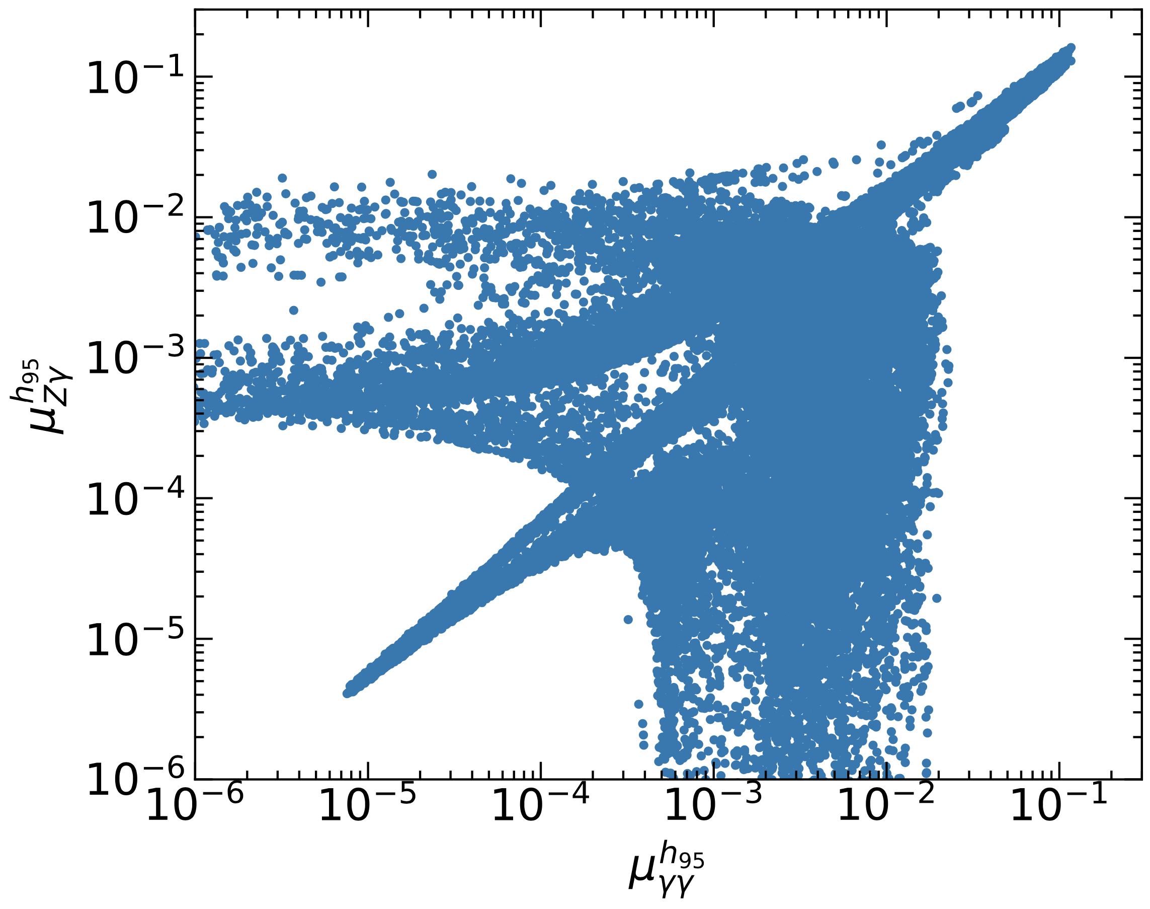
In Figure 4, we present the detailed correlation between signal strengths of and within the viable parameter space. In the left panel of Fig. 4, we show the viable parameter space spanned on the signal strengths of and plane. The signal strengths of and is presented in the right panel. Here, for both and , the production mode considered is gluon-gluon fusion. It is evident that the signal strengths of and exhibit a strong correlation, whereas this correlation is not observed for the boson.
V Conclusion
Recent results from low-mass Higgs boson searches at the LHC reveal excesses around GeV in the di-photon final state, with a local significance of combining both CMS and ATLAS data, and the di-tau final state, with a local significance of from CMS. An excess at similar mass with a local significance of was previously observed at the LEP experiment. Furthermore, the LHC has reported the first evidence of a rare decay mode of the 125 GeV Higgs boson into .
In this study, we have investigated the simultaneously interpretation of the excesses at GeV arising from the production of a lighter scalar boson and the rare decay mode of the Higgs boson into in the framework of gauged two-Higgs-doublet model.
We have presented an analysis of the decay properties of the lighter scalar boson . In addition to its decays into SM particles due to the mixing with SM Higgs boson, can decay into particles within the dark sector via its major hidden component, including DM, dark photons, and dark bosons, where kinematically feasible. The decay rate of to SM particles is significantly influenced by the mixing angle , with a larger value of correlating to higher decay rates. Notably, the channel emerges as the predominant decay mode among SM particle final states. On the other hand, the decay rate of into dark sector particles strongly depends on the new gauge couplings and the mass of the final state particles. For a substantial gauge coupling and a low mass region of DM, the branching ratios of decaying into dark sector particles can dominate, as illustrated in Fig. 1.
We focused our investigation on the di-photon and final states from the decays of both 95 GeV and 125 GeV Higgs bosons. In addition to the anticipated contributions from boson and SM fermions loops, our analysis found significant effects from charged Higgs loop, especially in low charged Higgs mass region. The impact of the hidden fermions loop remains negligible within our parameter range of interest. The signal strengths of and can either be enhanced or suppressed depending on the constructive or destructive interference between these contributions, as depicted in Fig. 2.
Employing an exhaustive parameter space scan, constrained by the theoretical conditions and experimental data, we present our main results in Fig. 3. We found that the viable parameter space in the model can simultaneously address the excesses observed around 95 GeV in the final state channel at LEP and the di-photon final state channel at the LHC as well as the recent evidence for the 125 GeV Higgs boson decay into at the LHC. On the other hand, the signal strength of is insufficient to account for the excess reported by CMS. Moreover, we found a strong correlation between the signal strengths of and , although this correlation doesn’t extend to the lighter scalar , as shown in Fig. 4.
Forthcoming results for the low-mass searches in di-tau final state channel from the ATLAS experiment, along with upcoming Run 3 results from both ATLAS and CMS, particularly for the di-photon final state channel, hold promise in shedding light on the potential presence of an addition scalar boson around 95 GeV.
Acknowledgments
This work was supported in part by the National Natural Science Foundation of China, grant Nos. 19Z103010239 and 12350410369 (VQT), the NSTC grant No. 111-2112-M-001-035 (TCY), and the Moroccan Ministry of Higher Education and Scientific Research MESRSFC and CNRST Project PPR/2015/6 (AB). VQT would like to thank the Medium and High Energy Physics group at the Institute of Physics, Academia Sinica, Taiwan for their hospitality during the course of this work.
Appendix A
The general analytical expressions for the one-loop amplitudes of the two processes and 111See for example Refs. Gunion et al. (2000); Gamberini et al. (1987); Weiler and Yuan (1989); Chen et al. (2013); Hue et al. (2018) for the computation of this process in a variety of BSM. in G2HDM were given in the Appendix in Tran et al. (2023a). To make this paper self-contained, we briefly summarize these formulas here. As mentioned in the text, , and are identified as the lighter scalar with mass GeV, the observed Higgs with mass GeV Sirunyan et al. (2020) and boson with mass GeV Zyla et al. (2020), respectively.
Define the following two well-known loop functions and Gunion et al. (2000)
| (39) | |||||
| (40) |
with
| (43) | |||||
| (46) |
where
| (47) |
Fig. 5 illustrates the loop functions for the process, multiplied by the phase space factor , as a function of . In this case, and , where represents the mass of the particle running inside the loop. We note that the loop function exhibits a singularity at ; however, this will be canceled out by the phase space factor. Furthermore, when the particle running inside the loop is on-shell (), the loop functions acquire imaginary parts, with the real parts peaking at the mass threshold ().


A.1 Decay Rate of
The partial decay rate for is
| (48) |
where with denotes the loop form factor for charged particle with spin equals respectively running inside the loop.
In G2HDM, the only charged spin 1 particle is the SM , thus ,
| (49) | |||||
Here and below, we denote and .
All the charged fermions in G2HDM, including both the SM fermions and the new heavy fermions contribute to . Thus
| (50) |
where
| (51) | |||||
and
| (52) | |||||
with being the color factor and the electric charge of in unit of ; the vector couplings of quarks and leptons are listed in Table 1 and Table 2 respectively.
There is only one charged Higgs in G2HDM. Thus with
| (53) | |||||
where , and and are the and couplings in the G2HDM respectively. Explicitly they are
| (54) | |||||
| (55) | |||||
A.2 Decay Rates of and
The partial decay rate for is
| (56) |
where , , where and denote summation over all charged SM and heavy hidden fermions, and with
| (57) | |||||
| (58) | |||||
| (59) | |||||
| (60) | |||||
The partial decay rate for is
| (61) |
where and
| (62) | |||||
| (63) | |||||
References
- CMS (2023) Search for a standard model-like Higgs boson in the mass range between 70 and 110 in the diphoton final state in proton-proton collisions at , Tech. Rep. (CERN, Geneva, 2023).
- (2) ATLAS, https://indico.cern.ch/event/1281604/ .
- ATL (2023) Search for diphoton resonances in the 66 to 110 GeV mass range using 140 fb-1 of 13 TeV collisions collected with the ATLAS detector, Tech. Rep. (CERN, Geneva, 2023) all figures including auxiliary figures are available at https://atlas.web.cern.ch/Atlas/GROUPS/PHYSICS/CONFNOTES/ATLAS-CONF-2023-035.
- Biekötter et al. (2023a) T. Biekötter, S. Heinemeyer, and G. Weiglein, (2023a), arXiv:2306.03889 [hep-ph] .
- CMS (2022) Searches for additional Higgs bosons and vector leptoquarks in final states in proton-proton collisions at , Tech. Rep. (CERN, Geneva, 2022).
- Barate et al. (2003) R. Barate et al. (LEP Working Group for Higgs boson searches, ALEPH, DELPHI, L3, OPAL), Phys. Lett. B 565, 61 (2003), arXiv:hep-ex/0306033 .
- Dev et al. (2023) P. S. B. Dev, R. N. Mohapatra, and Y. Zhang, (2023), arXiv:2312.17733 [hep-ph] .
- Li et al. (2023) W. Li, H. Qiao, K. Wang, and J. Zhu, (2023), arXiv:2312.17599 [hep-ph] .
- Chen et al. (2023) T.-K. Chen, C.-W. Chiang, S. Heinemeyer, and G. Weiglein, (2023), arXiv:2312.13239 [hep-ph] .
- Ahriche (2023) A. Ahriche, (2023), arXiv:2312.10484 [hep-ph] .
- Arcadi et al. (2023) G. Arcadi, G. Busoni, D. Cabo-Almeida, and N. Krishnan, (2023), arXiv:2311.14486 [hep-ph] .
- Ahriche et al. (2023) A. Ahriche, M. L. Bellilet, M. O. Khojali, M. Kumar, and A.-T. Mulaudzi, (2023), arXiv:2311.08297 [hep-ph] .
- Borah et al. (2023) D. Borah, S. Mahapatra, P. K. Paul, and N. Sahu, (2023), arXiv:2310.11953 [hep-ph] .
- Cao et al. (2023) J. Cao, X. Jia, J. Lian, and L. Meng, (2023), arXiv:2310.08436 [hep-ph] .
- Ellwanger and Hugonie (2023) U. Ellwanger and C. Hugonie, (2023), arXiv:2309.07838 [hep-ph] .
- Dutta et al. (2023) J. Dutta, J. Lahiri, C. Li, G. Moortgat-Pick, S. F. Tabira, and J. A. Ziegler, (2023), arXiv:2308.05653 [hep-ph] .
- Aguilar-Saavedra et al. (2023) J. A. Aguilar-Saavedra, H. B. Câmara, F. R. Joaquim, and J. F. Seabra, Phys. Rev. D 108, 075020 (2023), arXiv:2307.03768 [hep-ph] .
- Ashanujjaman et al. (2023) S. Ashanujjaman, S. Banik, G. Coloretti, A. Crivellin, B. Mellado, and A.-T. Mulaudzi, (2023), arXiv:2306.15722 [hep-ph] .
- Belyaev et al. (2023) A. Belyaev, R. Benbrik, M. Boukidi, M. Chakraborti, S. Moretti, and S. Semlali, (2023), arXiv:2306.09029 [hep-ph] .
- Escribano et al. (2023) P. Escribano, V. M. Lozano, and A. Vicente, Phys. Rev. D 108, 115001 (2023), arXiv:2306.03735 [hep-ph] .
- Azevedo et al. (2023) D. Azevedo, T. Biekötter, and P. M. Ferreira, JHEP 11, 017 (2023), arXiv:2305.19716 [hep-ph] .
- Biekötter et al. (2023b) T. Biekötter, S. Heinemeyer, and G. Weiglein, Phys. Lett. B 846, 138217 (2023b), arXiv:2303.12018 [hep-ph] .
- Iguro et al. (2022) S. Iguro, T. Kitahara, and Y. Omura, Eur. Phys. J. C 82, 1053 (2022), arXiv:2205.03187 [hep-ph] .
- Biekötter et al. (2022) T. Biekötter, S. Heinemeyer, and G. Weiglein, JHEP 08, 201 (2022), arXiv:2203.13180 [hep-ph] .
- Sachdeva and Sadhukhan (2020) D. Sachdeva and S. Sadhukhan, Phys. Rev. D 101, 055045 (2020), arXiv:1908.01668 [hep-ph] .
- He et al. (2024) X.-G. He, Z.-L. Huang, M.-W. Li, and C.-W. Liu, (2024), arXiv:2402.08190 [hep-ph] .
- Aad et al. (2024) G. Aad et al. (ATLAS, CMS), Phys. Rev. Lett. 132, 021803 (2024), arXiv:2309.03501 [hep-ex] .
- Huang et al. (2016a) W.-C. Huang, Y.-L. S. Tsai, and T.-C. Yuan, JHEP 04, 019 (2016a), arXiv:1512.00229 [hep-ph] .
- Arhrib et al. (2018) A. Arhrib, W.-C. Huang, R. Ramos, Y.-L. S. Tsai, and T.-C. Yuan, Phys. Rev. D 98, 095006 (2018), arXiv:1806.05632 [hep-ph] .
- Huang et al. (2019) C.-T. Huang, R. Ramos, V. Q. Tran, Y.-L. S. Tsai, and T.-C. Yuan, JHEP 09, 048 (2019), arXiv:1905.02396 [hep-ph] .
- Chen et al. (2020) C.-R. Chen, Y.-X. Lin, C. S. Nugroho, R. Ramos, Y.-L. S. Tsai, and T.-C. Yuan, Phys. Rev. D 101, 035037 (2020), arXiv:1910.13138 [hep-ph] .
- Huang et al. (2016b) W.-C. Huang, Y.-L. S. Tsai, and T.-C. Yuan, Nucl. Phys. B 909, 122 (2016b), arXiv:1512.07268 [hep-ph] .
- Chen et al. (2019) C.-R. Chen, Y.-X. Lin, V. Q. Tran, and T.-C. Yuan, Phys. Rev. D 99, 075027 (2019), arXiv:1810.04837 [hep-ph] .
- Huang et al. (2018) W.-C. Huang, H. Ishida, C.-T. Lu, Y.-L. S. Tsai, and T.-C. Yuan, Eur. Phys. J. C 78, 613 (2018), arXiv:1708.02355 [hep-ph] .
- Ramos et al. (2021a) R. Ramos, V. Q. Tran, and T.-C. Yuan, Phys. Rev. D 103, 075021 (2021a), arXiv:2101.07115 [hep-ph] .
- Ramos et al. (2021b) R. Ramos, V. Q. Tran, and T.-C. Yuan, JHEP 11, 112 (2021b), arXiv:2109.03185 [hep-ph] .
- Tran et al. (2023a) V. Q. Tran, T. T. Q. Nguyen, and T.-C. Yuan, Eur. Phys. J. C 83, 346 (2023a), arXiv:2208.10971 [hep-ph] .
- Tran and Yuan (2023) V. Q. Tran and T.-C. Yuan, JHEP 02, 117 (2023), arXiv:2212.02333 [hep-ph] .
- Liu et al. (2024) C. H. Liu, V. Q. Tran, Q. Wen, F. Xu, and T.-C. Yuan, (2024), arXiv:2404.06397 [hep-ph] .
- Dirgantara and Nugroho (2022) B. Dirgantara and C. S. Nugroho, Eur. Phys. J. C 82, 142 (2022), arXiv:2012.13170 [hep-ph] .
- Tran et al. (2023b) V. Q. Tran, T. T. Q. Nguyen, and T.-C. Yuan, (2023b), arXiv:2312.10785 [hep-ph] .
- Zyla et al. (2020) P. A. Zyla et al. (Particle Data Group), PTEP 2020, 083C01 (2020).
- Sirunyan et al. (2020) A. M. Sirunyan et al. (CMS), Phys. Lett. B 805, 135425 (2020), arXiv:2002.06398 [hep-ex] .
- Kilian et al. (1996) W. Kilian, M. Kramer, and P. M. Zerwas, Phys. Lett. B 373, 135 (1996), arXiv:hep-ph/9512355 .
- Fleischer and Jegerlehner (1983) J. Fleischer and F. Jegerlehner, Nucl. Phys. B 216, 469 (1983).
- Denner et al. (1992) A. Denner, J. Kublbeck, R. Mertig, and M. Bohm, Z. Phys. C 56, 261 (1992).
- Kniehl (1992) B. A. Kniehl, Z. Phys. C 55, 605 (1992).
- Sun et al. (2017) Q.-F. Sun, F. Feng, Y. Jia, and W.-L. Sang, Phys. Rev. D 96, 051301 (2017), arXiv:1609.03995 [hep-ph] .
- Bondarenko et al. (2019) S. Bondarenko, Y. Dydyshka, L. Kalinovskaya, L. Rumyantsev, R. Sadykov, and V. Yermolchyk, Phys. Rev. D 100, 073002 (2019), arXiv:1812.10965 [hep-ph] .
- Heng et al. (2015) Z.-X. Heng, D.-W. Li, and H.-J. Zhou, Commun. Theor. Phys. 63, 188 (2015).
- Abouabid et al. (2021) H. Abouabid, A. Arhrib, R. Benbrik, J. El Falaki, B. Gong, W. Xie, and Q.-S. Yan, JHEP 05, 100 (2021), arXiv:2009.03250 [hep-ph] .
- Aiko et al. (2021) M. Aiko, S. Kanemura, and K. Mawatari, Eur. Phys. J. C 81, 1000 (2021), arXiv:2109.02884 [hep-ph] .
- Greco et al. (2018) M. Greco, G. Montagna, O. Nicrosini, F. Piccinini, and G. Volpi, Phys. Lett. B 777, 294 (2018), arXiv:1711.00826 [hep-ph] .
- Achard et al. (2003) P. Achard et al. (L3), Phys. Lett. B 575, 208 (2003), arXiv:hep-ex/0309056 .
- Aad et al. (2021) G. Aad et al. (ATLAS), Eur. Phys. J. C 81, 1118 (2021), arXiv:2106.01676 [hep-ex] .
- Tumasyan et al. (2022a) A. Tumasyan et al. (CMS), JHEP 04, 147 (2022a), arXiv:2106.14246 [hep-ex] .
- CMS (2020) Combined Higgs boson production and decay measurements with up to 137 fb-1 of proton-proton collision data at sqrts = 13 TeV, Tech. Rep. (CERN, Geneva, 2020).
- Tumasyan et al. (2022b) A. Tumasyan et al. (CMS), Phys. Rev. D 105, 092007 (2022b), arXiv:2201.11585 [hep-ex] .
- Aad et al. (2019) G. Aad et al. (ATLAS), Phys. Lett. B 796, 68 (2019), arXiv:1903.06248 [hep-ex] .
- Fabbrichesi et al. (2020) M. Fabbrichesi, E. Gabrielli, and G. Lanfranchi, (2020), 10.1007/978-3-030-62519-1, arXiv:2005.01515 [hep-ph] .
- Aghanim et al. (2020) N. Aghanim et al. (Planck), Astron. Astrophys. 641, A6 (2020), [Erratum: Astron.Astrophys. 652, C4 (2021)], arXiv:1807.06209 [astro-ph.CO] .
- Angloher et al. (2017) G. Angloher et al. (CRESST), Eur. Phys. J. C 77, 637 (2017), arXiv:1707.06749 [astro-ph.CO] .
- Agnes et al. (2018) P. Agnes et al. (DarkSide), Phys. Rev. Lett. 121, 081307 (2018), arXiv:1802.06994 [astro-ph.HE] .
- Agnes et al. (2023) P. Agnes et al. (DarkSide-50), Phys. Rev. D 107, 063001 (2023), arXiv:2207.11966 [hep-ex] .
- Aprile et al. (2018) E. Aprile et al. (XENON), Phys. Rev. Lett. 121, 111302 (2018), arXiv:1805.12562 [astro-ph.CO] .
- Aprile et al. (2019) E. Aprile et al. (XENON), Phys. Rev. Lett. 123, 251801 (2019), arXiv:1907.11485 [hep-ex] .
- Aprile et al. (2023) E. Aprile et al. (XENON), Phys. Rev. Lett. 131, 041003 (2023), arXiv:2303.14729 [hep-ex] .
- Meng et al. (2021) Y. Meng et al. (PandaX-4T), Phys. Rev. Lett. 127, 261802 (2021), arXiv:2107.13438 [hep-ex] .
- Aalbers et al. (2023) J. Aalbers et al. (LZ), Phys. Rev. Lett. 131, 041002 (2023), arXiv:2207.03764 [hep-ex] .
- Foreman-Mackey et al. (2013) D. Foreman-Mackey, D. W. Hogg, D. Lang, and J. Goodman, Publ. Astron. Soc. Pac. 125, 306 (2013), arXiv:1202.3665 [astro-ph.IM] .
- Gunion et al. (2000) J. F. Gunion, H. E. Haber, G. L. Kane, and S. Dawson, The Higgs Hunter’s Guide, Vol. 80 (2000).
- Gamberini et al. (1987) G. Gamberini, G. F. Giudice, and G. Ridolfi, Nucl. Phys. B 292, 237 (1987).
- Weiler and Yuan (1989) T. J. Weiler and T.-C. Yuan, Nucl. Phys. B 318, 337 (1989).
- Chen et al. (2013) C.-S. Chen, C.-Q. Geng, D. Huang, and L.-H. Tsai, Phys. Rev. D 87, 075019 (2013), arXiv:1301.4694 [hep-ph] .
- Hue et al. (2018) L. T. Hue, A. B. Arbuzov, T. T. Hong, T. P. Nguyen, D. T. Si, and H. N. Long, Eur. Phys. J. C 78, 885 (2018), arXiv:1712.05234 [hep-ph] .