When Do Curricula Work in Federated Learning?
Abstract
An oft-cited open problem of federated learning is the existence of data heterogeneity at the clients. One pathway to understanding the drastic accuracy drop in federated learning is by scrutinizing the behavior of the clients’ deep models on data with different levels of ”difficulty”, which has been left unaddressed. In this paper, we investigate a different and rarely studied dimension of FL: ordered learning. Specifically, we aim to investigate how ordered learning principles can contribute to alleviating the heterogeneity effects in FL. We present theoretical analysis and conduct extensive empirical studies on the efficacy of orderings spanning three kinds of learning: curriculum, anti-curriculum, and random curriculum. We find that curriculum learning largely alleviates non-IIDness. Interestingly, the more disparate the data distributions across clients the more they benefit from ordered learning. We provide analysis explaining this phenomenon, specifically indicating how curriculum training appears to make the objective landscape progressively less convex, suggesting fast converging iterations at the beginning of the training procedure. We derive quantitative results of convergence for both convex and nonconvex objectives by modeling the curriculum training on federated devices as local SGD with locally biased stochastic gradients. Also, inspired by ordered learning, we propose a novel client selection technique that benefits from the real-world disparity in the clients. Our proposed approach to client selection has a synergic effect when applied together with ordered learning in FL.
1 Introduction
Inspired by the learning principle underlying the cognitive process of humans, curriculum learning (CL) generally proposes a training paradigm for machine learning models in which the difficulty of the training task is progressively scaled, going from ”easy” to ”hard”. Prior empirical studies have demonstrated that CL is effective in avoiding bad local minima and in improving the generalization results [bengio-curriculum, SPL-curriculum-2015]. Also interestingly, another line of work proposes the exact opposite strategy of prioritizing the harder examples first, such as [curriculum-anti-2016-ijcai, anti-is-better-2018, anti-is-better-2019]–these techniques are referred to as “anti-curriculum”. It is shown that certain tasks can benefit from anti-curriculum techniques. However, in tasks such as object detection [ST3D-object-detection, curriculum-object-detection-2018-sangineto], and large-scale text models [curriculum-text-2020] CL is standard practice.
Although the empirical observations on CL appear to be in conflict, this has not impeded the study of CL in machine learning tasks. Certain scenarios [curriculum-Neyshabur-2021] have witnessed the potential benefits of CL. The efficacy of CL has been explored in a considerable breadth of applications, including, but not limited to, supervised learning tasks within computer vision [CurriculumNet-2018], healthcare [curriculum-federated-2021], reinforcement learning tasks [curriculum-Reinforcement-learning-2018], natural language processing (NLP) [curriculum-nlp-2019] as well as other applications such as graph learning [curriculum-graph-2019], and neural architecture search [curriculum-NAS-2020].
Curriculum learning has been studied in considerable depth for the standard centralized training settings. However, to the best of our knowledge, our paper is the first attempt at studying the methodologies, applications, and efficacy of CL in a decentralized training setting and in particular for federated learning (FL). In FL, the training time budget and the communication bandwidth are the key limiting constraints, and as demonstrated in [curriculum-Neyshabur-2021] CL is particularly effective in settings with a limited training budget. It is an interesting proposition to apply the CL idea to an FL setting, and that is exactly what we explore in our paper (in Section 2).
The idea of CL is agnostic to the underlying algorithms used for federation and hence can be very easily applied to any of the state-of-the-art solutions in FL. Our technique does not require a pre-trained expert model and does not impose any additional synchronization overhead on the system. Also, as the CL is applied to the client, it does not add any additional computational overhead to the server.
Further, we propose a novel framework for efficient client selection in an FL setting that builds upon our idea of CL in FL. We show in Section 4, CL on clients is able to leverage the real-world discrepancy in the clients to its advantage. Furthermore, when combined with the primary idea of CL in FL, we find that it provides compounding benefits.
Contributions: In this paper, we comprehensively assess the efficacy of CL in FL and provide novel insights into the efficacy of CL under the various conditions and methodologies in the FL environment.
We provide a rigorous convergence theory and analysis of FL in non-IID settings, under strongly convex and non-convex assumptions, by considering local training steps as biased SGD, where CL naturally grows the bias over the iterations, in Section LABEL:analysis-main-paper of the main paper and Section LABEL:sec:analysis of the Supplementary Material (SM).
We hope to provide comprehensible answers to the following six important questions:
Q1: Which of the curriculum learning paradigm is effective in FL? And under what conditions?
Q2: Can CL alleviate the statistical data heterogeneity in FL?
Q3: Does the efficacy of CL in FL depend on the underlying client data distributions?
Q4: Whether the effectiveness of CL is correlated with the size of datasets owned by each client?
Q5: Are there any benefits of smart client selection? And can CL be applied to the problem of client selection?
Q6: Can we apply the ideas of CL to both the client data and client selection?
We test our ideas on two widely adopted network architectures on popular datasets in the FL community (CIFAR-10, CIFAR-100, and FMNIST) under a wide range of choices of curricula and compare them with several global state-of-the-art baselines. We have the following findings:
- •
-
•
The efficacy of CL is more pronounced when the client data is heterogeneous (Section 3.3).
-
•
CL on client selection has a synergic effect that compounds the benefits of CL in FL (Section 4).
-
•
CL can alleviate data heterogeneity across clients and CL is particularly effective in the initial stages of training as the larger initial steps of the optimization are done on the “easier” examples which are closer together in distribution (Section LABEL:analysis-main-paper of main paper, and Section LABEL:sec:analysis of the SM).
-
•
The efficacy of our technique is observed in both lower and higher data regimes (Section LABEL:Effect-of-amount-of-data of the SM).
2 Curriculum Components
Federated Learning (FL) techniques provide a mechanism to address the growing privacy and security concerns associated with data collection, all-the-while satiating the need for large datasets for training powerful machine learning models. A major appeal of FL is its ability to train a model over a distributed dataset without needing the data to be collated into a central location for training. In the FL framework, we have a server and multiple clients with a distributed dataset. The process of federation is an iterative process that involves multiple rounds of back-and-forth communication between the server and the clients that participate in the process [Vahidian-rethinking-2022-workshop]. This back-and-forth communication incurs a significant communication overhead, thereby limiting the number of rounds that are pragmatically possible in real-world applications. Curriculum learning is an idea that particularly shines in these scenarios where the training time is limited [curriculum-Neyshabur-2021]. Motivated by this idea, we define a curriculum for training in the federated learning setting. A curriculum consists of three key components:
The scoring function: It is a mapping from an input sample, , to a numerical value, . We define a range of scoring functions when defining a CL for the FL setting in the subsequent sections. When defining the scoring function of a curriculum in FL, we look for loss-based dynamic measures for the score that update every iteration, unlike the methods proposed in [curriculum-cscore-2020] which produce a fixed score for each sample. This is because the instantaneous score of samples changes significantly between iterations, and using a fixed score leads to an inconsistency in the optimization objectives, making training less stable [curriculum-DIH-bilmes-2020]. Also, we avoid techniques like [curriculum-humna-score-2015] which requires human annotators, as it is not practical in a privacy-preserving framework.
The pacing function: The pacing function determines scaling of the difficulty of the training data introduced to the model at each of the training steps and it selects the highest scoring samples for training at each step. The pacing function is parameterized by where is the fraction of the training budget needed for the pacing function to begin sampling from the full training set and represents the fraction of the training set the pacing function exposes to the model at the start of training. In this paper, the full training set size and the total number of training steps (budget) are denoted by and , respectively. Further, we consider five pacing function families, including exponential, step, linear, quadratic, and root (sqrt). The expressions we used for the pacing functions are shown in Table LABEL:tab:pacing-formula of the SM. we follow [curriculum-power-of-2019] in defining the notion of pacing function and use it to schedule how examples are introduced to the training procedure.
The order: Curriculum learning orders sample from the highest score (easy ones) to lowest score, anti-curriculum learning orders from lowest score to highest, and finally, random curriculum randomly samples data in each step regardless of their scores.
3 Experiment
Experimental setting. To ensure that our observations are robust to the choice of architectures, and datasets, we report empirical results for LeNet-5 [lecun1989backpropagation] architecture on CIFAR-10 [krizhevsky2009learning] and Fashion MNIST (FMNIST) [xiao2017fashion], and ResNet-9 [he2016deep] architecture for CIFAR-100 [krizhevsky2009learning] datasets. All models were trained using SGD with momentum. Details of the implementations, architectures, and hyperparameters can be found in Section LABEL:impelement-detail of the SM.
Baselines and Implementation. To provide a comprehensive study on the efficacy of CL on FL setups, we consider the predominant approaches to FL that train a global model, including FedAvg [mcmahan2017communication], FedProx [fedprox-smith-2020], SCAFFOLD [scaffold-2020], and FedNova [FedNova-2020]. In all experiments, we assume 100 clients are available, and 10 of them are sampled randomly at each round. Unless stated otherwise, throughout the experiments, the number of communication rounds is 100, each client performs 10 local epochs with a batch size of 10, and the local optimizer is SGD. To better understand the mutual impact of different data partitioning methods in FL and CL, we consider both federated heterogeneous (Non-IID) and homogeneous (IID) settings. In each dataset other than IID data partitioning settings, we consider two different federated heterogeneity settings as in [vahidian-pacfl-2022, Vahidian-FLIS-2022]: Non-IID label skew (), and Non-IID Dir.
3.1 Effect of scoring function in IID and Non-IID FL
In this section, we investigate five scoring functions. As discussed earlier, in standard centralized training, samples are scored using the loss value of an expert pre-trained model. Given a pre-trained model , the score is defined as , where , with being the inference loss. In this setup, a higher score corresponds to an easier sample.
In FL [mcmahan2017communication, Vahidian-federated-2021], a trusted server broadcasts a single initial global model, , to a random subset of selected clients in each round. The model is optimized in a decentralized fashion by multiple clients who perform some steps of SGD updates . The resulting model is then sent back to the server, ultimately converging to a joint representative model. With that in mind, in our setting, the scores can be obtained by clients either via the global model that they receive from the server, which we name as or by their own updated local model, named as or the score can be determined based on the average of the local and global model loss, named as 111Since it produces very similar results to , we skipped it..
We further consider another family of scoring that is based on ground truth class prediction. In particular, in each round, clients receive the global model from the server and get the prediction using the received global model and the current local model as and , respectively. For those samples whose and do not match, the client tags them as hard samples and otherwise as easy ones. This scoring method is called . Further, ground truth class prediction and scoring can be solely done by the global model or the client’s local model, which end up with two other different scoring methods, namely , and respectively. This procedure is described in Algorithm 1.
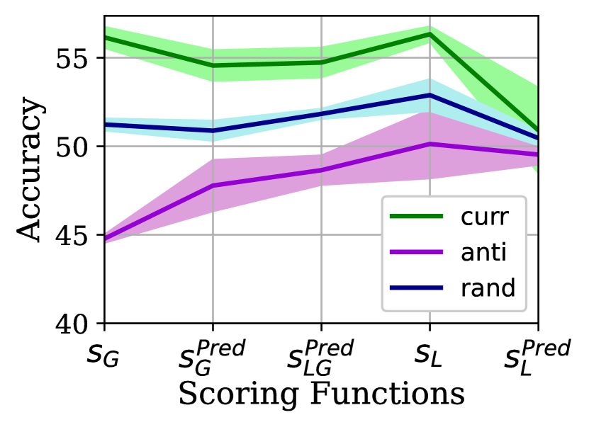
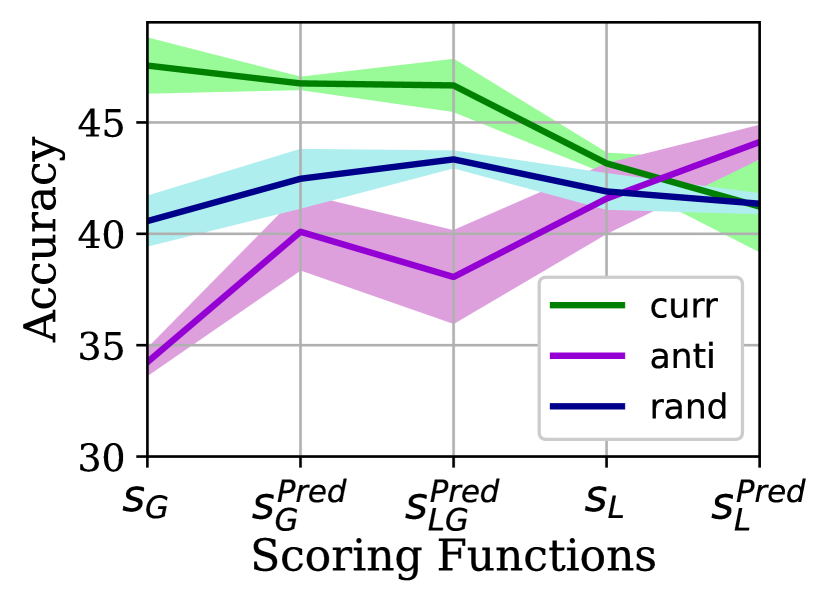
Fig. 1 demonstrates what the impact of using these various scoring methods is on the global accuracy when curriculum, anti-curriculum, or random ordering is exploited by the clients in the order in which their CIFAR-10 examples are learned with FedAvg under IID and Non-IID (2) data partitions. The results are obtained by averaging over three randomly initialized trials and calculating the standard deviation (std).
The results reveal that first, the scoring functions are producing broadly consistent results except for for both IID and Non-IID and for Non-IID settings. provides the most accurate scores, thereby improving the accuracy by a noticeable margin compared to its peers. This is quite expected, as the global model is more mature compared to the client model, second, the curriculum learning improves the accuracy results consistently across different scoring functions, third, curriculum learning is more effective when the clients underlying data distributions are Non-IID. To ensure that the latter does not occur by chance, we will delve into this point in detail in subsection 3.3. Due to the superiority of relative to others, we set the scoring function to be henceforth. We will further elaborate on the precision of compared to an expert model in Section LABEL:expert-G-compare.
3.2 Effect of pacing function and its parameters in IID and Non-IID FL
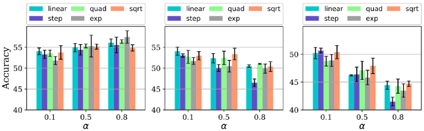
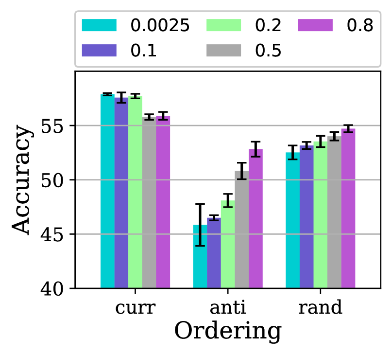
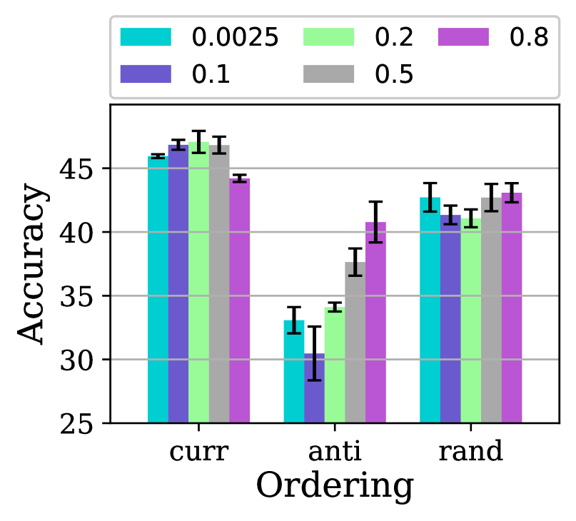
In order to study the effect of different families of pacing functions along with the hyperparameters , we test the exponential, step, linear, quadratic, and root function families. We further first fix to and let 222Note that . Also, or is equivalent to no ordered training, i.e., standard training.. The accuracy results are presented in Fig. 2. It is noteworthy that the complement of this figure for Non-IID is presented in Fig. LABEL:pacing-a-cifar10-iid-ordering in the SM. As is evident, for all pacing function families, the trends between the curriculum and the other orderings, i.e., (anti, random)-curriculum are markedly opposite in how they improve/degrade by sweeping from small values to large ones. The pattern for Non-IID which presented in the SM is almost similar to that of IID. Values of produce the best results. As can be seen from Fig. 2, the best accuracy achieved by curriculum learning outperforms the best accuracy obtained by other orderings by a large margin. For example, in the “linear” pacing function, the best accuracy achieved for curriculum learning when is which improved the vanilla results by while that of random when is and improved vanilla by . Henceforth, we set and the pacing function to linear. After selecting the pacing function and the final step is to fix these two and see the impact of . Now we let all curricula use the linear pacing functions with a = 0.8 and only sweep and report the results in Fig. 3. Perhaps most striking is that curriculum learning tends to have smaller values of to improve accuracy, which is in contrast with (random-/anti) orderings. The performance of anti-curriculum shows a significant dependence on the value of . Further, curriculum learning provides a robust benefit for different values of and it beats the vanilla FedAvg by depending upon the distribution of the data. Henceforth, we fix to .
3.3 Effect of level of data heterogeneity
Equipped with the ingredients explained in the preceding section, we are now in a position to investigate the significant benefits of employing curriculum learning in FL when the data distribution environment is more heterogeneous. To ensure a reliable finding, we investigate the impact of heterogeneity in four baselines through extensive experiments on benchmark datasets, i.e., CIFAR-10, CIFAR-100, and FMNIST. In particular, we distribute the data between clients according to Non-IID Dir defined in [li2021federated]. In Dir, heterogeneity can be controlled by the parameter of the Dirichlet distribution. Specifically, when the clients’ data partitions become IID, and when they become extremely Non-IID.
To understand the relationship between the ordering-based learning and the level of statistical data heterogeneity, we ran all baselines for different Dirichlet distribution values . The accuracy results of different baselines on CIFAR-10 while employing (anti-) curriculum, or random learning with linear pacing functions and using are presented in Tables 1, 2, 3, and 4. For the comprehensiveness of the study, we will present results for CIFAR-100 respectively in Section LABEL:cifar-100-effect-of-level-hetero of the SM.
The results are surprising: The benefits of ordered learning are more prominent with increased data heterogeneity. The greater the distribution discrepancy between clients, the greater the benefit to curriculum learning.
If we consider client heterogeneity as distributional skew[zhu2021federated], then this is logical: easier data samples are those with overall lower variance, both unbiased and skew from the mean, and thus the total collection of CL-easier data samples in a dataset is more IID than the alternative. Thus, in the crucial early phases of training, the training behaves closer to FedAvg/FedProx/SCAFFOLD/FedNova under IID distributions. Therefore, CL can alleviate the drastic accuracy drop when clients’ decentralized data are statistically heterogeneous, which comes from stable training from IID samples to Non-IID ones, fundamentally improving the accuracy. This is formalized with quantitative convergence rates in the Section LABEL:analysis-main-paper of the main paper and in Section LABEL:sec:analysis of the SM.
| Non-IIDness | Curriculum | Anti | Random | Vanilla |
| Dir() | ||||
| Dir() | ||||
| Dir() |
| Non-IIDness | Curriculum | Anti | Random | Vanilla |
| Dir() | ||||
| Dir() | ||||
| Dir() |
| Non-IIDness | Curriculum | Anti | Random | Vanilla |
| Dir() | ||||
| Dir() | ||||
| Dir() |
| Non-IIDness | Curriculum | Anti | Random | Vanilla |
| Dir() | ||||
| Dir() | ||||
| Dir() |
4 Curriculum on Clients
The technique of ordered learning presented in previous sections is designed to exploit the heterogeneity of data at the clients but is not geared to effectively leverage the heterogeneity between the clients that, as we discuss further, naturally emerges in the real world.
In the literature, some recent works have dabbled with the idea of smarter client selection, and many selection criteria have been suggested, such as importance sampling, where the probabilities for clients to be selected are proportional to their importance measured by the norm of update [Optimal-Client-Sampling-2022], test accuracy [client-selection-iot-2021]. The [power-of-choice-2020] paper proposes client selection based on local loss where clients with higher loss are preferentially selected to participate in more rounds of federation, which is in stark contrast to [client-selection-2022-curr] in which the clients with a lower loss are preferentially selected. It’s clear from the literature that the heterogeneous environment in FL can hamper the overall training and convergence speed [haddadpour2019convergence, mahdavi2020-APFL], but the empirical observations on client selection criteria are either in conflict or their efficacy is minimal. In this section, inspired by curriculum learning, we try to propose a more sophisticated mechanism of client selection that generalizes the above strategies to the FL setting.
4.1 Motivation
In the real world, the distributed dataset used in FL is often generated in-situ by clients, and the data is measured/generated using a particular sensor belonging to the client. For example, consider the case of a distributed image dataset generated by smartphone users using the onboard camera or a distributed medical imaging dataset generated by hospitals with their in-house imaging systems. In such scenarios, as there is a huge variety in the make and quality of the imaging sensors, the data generated by the clients is uniquely biased by the idiosyncrasies of the sensor, such as the noise, distortions, quality, etc. This introduces variability in the quality of the data at clients, in addition to the Non-IID nature of the data. However, it is interesting to note that these effects apply consistently across all the data at the specific client.
From a curriculum point of view, as the data points are scored and ordered by difficulty, which is just a function of the loss value of that data point, these idiosyncratic distortions uniformly affect the loss/difficulty value of all the data at that particular client. Also, it is possible that the difficulty among the data points at the particular client is fairly consistent as the level of noise, quality of the sensor, etc. are the same across the data points. This bias in difficulty varies between clients but is often constant within the same client. Naturally, this introduces a heterogeneity in the clients participating in the federation. In general, this can be thought of as some clients being ”easy” and some being ”difficult”. We can quantify this notion of consistency in difficulty by the standard deviation in the score of the data points at the client.
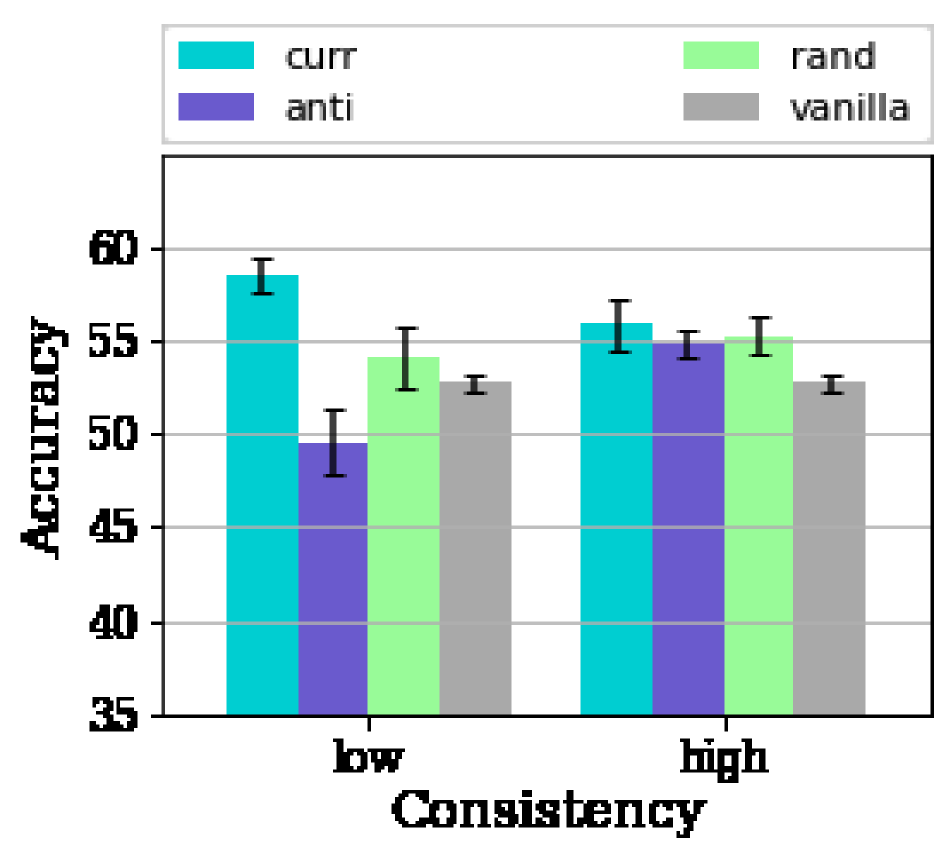
When the standard deviation of the intra-client data is low, i.e., when the difficulty of the data within a client is consistent, we find that the curriculum on FL behaves very differently in these kinds of scenarios. We observe the advantage of curriculum diminishes significantly and has similar efficacy as that of random curricula as shown in Fig 4. The advantage of curriculum can be defined as , where .
4.2 Client Curriculum
We propose to extend the ideas of curriculum onto the set of clients, in an attempt to leverage the heterogeneity in the clients. To the best of our knowledge, our paper is the first attempt to introduce the idea of curriculum on clients in an FL setting. Many curricula ideas can be neatly extended to apply to the set of clients. In order to define a curriculum over the clients, we need to define a scoring function, a pacing function, and an ordering over the scores. We define the client loss as the mean loss of the local data points at the client (Eq. 1), and the client score can be thought of as inversely proportional to the loss. The ordering is defined over the client scores.
| (1) |
where is the index for client, represents the dataset at client , is the loss of th data point in .
The pacing function, as in the case of data curricula, is used to pace the number of clients participating in the federation. Starting from a small value, the pacing function gradually increases the number of clients participating in the federation. The action of the pacing function amounts to scaling the participation rate of the clients.
The clients are scored and rank-ordered based on the choice of ordering, then a subset of size of the clients is chosen in a rank-ordered fashion. The value is prescribed by the pacing function. The clients are randomly batched into mini-batches of clients. These mini-batches of clients subsequently participate in the federation process. Thereby, we have two sets of curricula, one that acts locally on the client data and the other that acts on the set of clients. Henceforth we will refer to these as the data curriculum and the client curriculum, respectively. We study the interplay of these curricula in Section LABEL:sec:ablation_study.
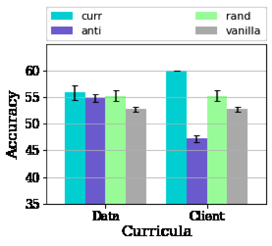
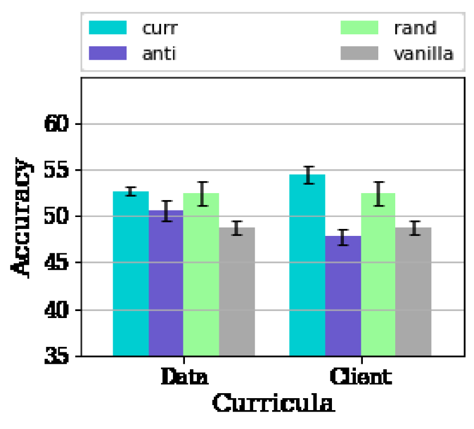
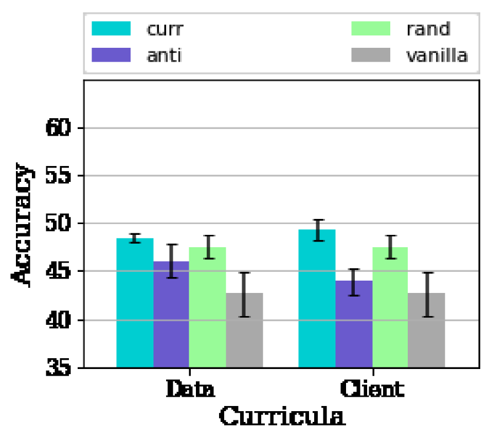
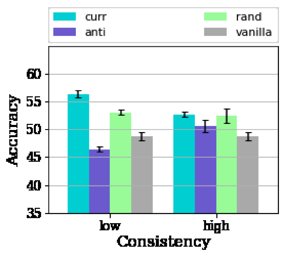
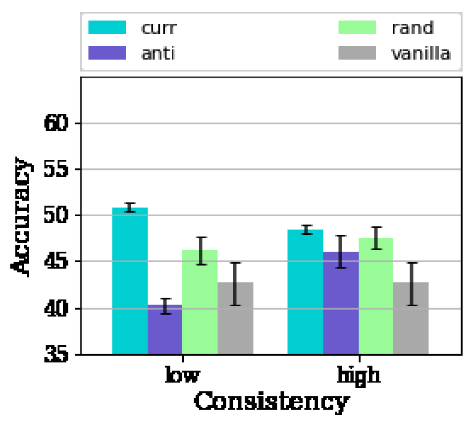
Fig. 5 confirms that the benefits of the algorithm severely depend on the data of the client having a diverse set of difficulties. As is evident from Fig. 5, we are able to realize an of % for the different values of Non-IIDness using our proposed client curriculum algorithm in the scenario with high consistency in the client data where the data curriculum has reduced/no benefits. This illustrates that the client curriculum is able to effectively overcome the limiting constraint of local variability in data and is able to leverage the heterogeneity in the set of clients to its benefit.
4.3 Difficulty based partitioning
For the experiments in this section, we require client datasets () of varying difficulty at the desired level of Non-IIDness. In order to construct partitions of varying difficulty, we need to address two key challenges: one, we need a way to accurately assess the difficulty of each of the data points, and two, we need to be able to work with different levels of Non-IIDness. To address the first challenge, we rank the data points in order of difficulty using an a priori trained expert model that was trained on the entire baseline dataset and has the same network topology as the global model. As the expert model has the same topology as the model that we intend to train and as it is trained on the entire dataset, it is an accurate judge of the difficulty of the data points. Interestingly, this idea can be extended to be used as a scoring method for curriculum as well. We call this scoring method the expert scoring . We look at this in greater detail in Section LABEL:expert-G-compare.
To address the second challenge, a possible solution is to first partition the standard dataset into the desired Non-IID partitions using well-known techniques such as the Dirichlet distribution, followed by adding different levels of noise to the samples of the different data partitions. This would partition with varying difficulty; however, doing so would alter the standard baseline dataset, and we would lose the ability to compare the results to known baseline values and between different settings. We would like to be able to compare our performance results with standard baselines, so we require a method that does not alter the data or resort to data augmentation techniques, and we devise a technique that does just that.
Starting with the baseline dataset, we first divide it into the desired Non-IID partitions the same as before, but then instead of adding noise to the dataset, we attempt to reshuffle the data among partitions in such a way that we create ”easy” partitions and ”hard” partitions. This can be achieved by ordering the data in increasing order of difficulty and distributing the data among the partitions starting from the ”easy” data points, all the while honoring the Non-IID class counts of each of the partitions as determined by the Non-IID distribution. The outline is detailed in Algorithm 2. It is noteworthy that, although we are able to generate partitions of varying difficulty, we do not have direct control over the ”difficulty” of each of the partitions and hence cannot generate partitions with an arbitrary distribution of difficulty as can be done by adding noise.