What can we learn from the experiment of electrostatic conveyor belt for excitons?

According to the above analysis, there are various sources for the coherent excitons. As a result, the initial distribution of the degenerate excitons can be considered as a wave pocket with multi-peaks. In order to understand the transport of the wave pocket, let us first study the simplest case of the diffusion of a wave pocket with one-peak. We solve the time-dependent nonlinear Schrödinger equation (1) in real-time only under the open boundary condition ($\psi_{\pm L}=0$) for an initial Gauss wave pocket $\psi_{j}(0)=\sqrt{(2\kappa/\pi)}\exp\left[-\kappa(j-j_{0})^{2}\right]$. The results with the parameters $j_{0}=-16$, $\kappa=0.006$ and $L=128$ are shown in Fig. 2. In the following discussions, the blue lines in all the figures indicate the shape of the initial wave pocket.

The physics of the wave pocket diffusion is very simple Zeng (2007); Sakurai (1994). For the Gauss wave pocket, its wave functions both in real space and momentum space are all of the Gauss type. According to the uncertainty relation $\Delta x\Delta p\approx\hbar$, with the increase of time, the larger $\Delta x$ leads to the smaller $\Delta p$, here $\Delta x$ and $\Delta p$ are the full width at half maximum of the Gauss wave pocket. If we approximately take $v\approx\Delta v$, the smaller $\Delta p$ leads to the lower the propagation speed. As a result, although the diffusion becomes slower and slower as the time increases, the wave finally arrives at the boundary and is reflected. Interference fringes are generated by the interference between reflected and incident waves. The above statements are true whether it is without the periodic potential in Fig. 2 (a) or with the static periodic potential in Fig. 2 (d). The difference is that more interference fringes appear in Fig. 2 (d) due to the interplay between the wave and the periodic potential. When we take the dissipation of the particles into account, the wave pocket decays in Fig. 2 (b) and (e) with the time goes on. The escape probability $I_{j}$ in Eq. (5) is calculated and shown in Fig. 2 (c) and (f). As expected, the particle dissipation suppresses the wave pocket diffusion. From Fig. 2 (f), $I_{j}$ can be deviated from the initial position due to the modulation of the external potential.

We next investigate the cooling effect on the wave pocket diffusion. The time-dependent nonlinear Schrödinger equation (1) is solved with the real-time and imaginary-time evolutions alternatively to obtain the escape rate $I_{j}$ of the coherent excitons. The result of $I_{j}$ is shown in Fig. 3. It can be seen that the cooling helps the wave pocket diffusion. We can understand the underlying physical picture as follow Zeng (2007); Sakurai (1994). A wave pocket in free space can be considered as the superposition of the plane waves with the different wave vectors. When the condensed Bosons are considered to be in a state of Gauss wave pocket in momentum space, their distribution in the Cartesian coordinate space is still Gauss type. With the time increases, the wave pocket will spread in coordinate space and will contract in momentum space. However, their waves are still Gauss types. With the temperature decreases, the low-energy probability of the Gauss wave pocket increases accordingly since the wave pocket in momentum space is modulated by the factor $\exp(-\beta E_{k})$ ($E_{k}=k^{2}/2$). The narrower the wave pocket in momentum space, the wider wave pocket in coordinate space Zeng (2007); Sakurai (1994). As a result, the quantum mechanical effect is in opposition to the classical effect where the spreading of classical particle becomes slow with the decrease of the temperature.

By comparing the black lines and the red lines in Fig. 3 (b), it is found that the cooling also helps the wave pocket spread in a static periodic potential. The physical picture can also be understood in a similar way. In the static periodic potential, the eigenfunction of a particle is the Bloch wave which can be expanded in terms of the Wannier functions. Correspondingly, the energy bands come from the splitting of the degenerate energy levels. A wave pocket in periodic potential can be considered as a superposition of the Bloch waves with the different wave vectors. With time increasing and particle cooling, the particle probabilities in low-energy bands increase accordingly. The narrower the wave pocket in momentum space, the wider the wave pocket in coordinate space. As a result, the cooling enhances the diffusion of the wave pocket.

It is interesting to see in Fig. 3 (c) that the peaks of the $I_{j}$ for $\tau>0$ are located at the crests of the periodic potential, which is in contrast to the case of $\tau=0$ where the peaks are located at the troughs. The reason can be understood as follows. According to the above analysis, with the lowering of the temperature, the Bosons tend to condense at $k=0$, which results in the increasing of $\Delta x$. In the large $A_{\text{conv}}$ case, the Wannier functions are the atomic orbital wavefunctions in a unit cell and the particles are confined in a single unit cell. The stronger the confinement, the larger the $\Delta x$. The particles tend to move to the boundary of the unit cell to obtain the large $\Delta x$ which causes the dip of particle distribution at the center of the unit cell. This quantum behavior can be used to detect the exciton degeneracy.

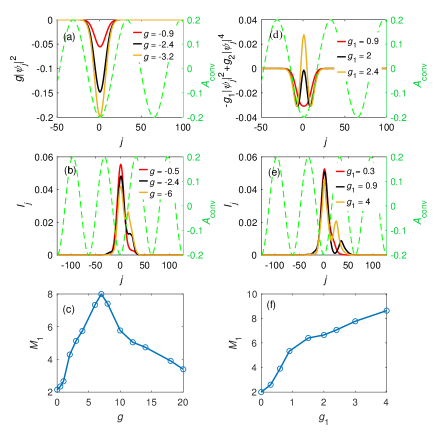
The wave pocket diffusion in a moving lattice is shown in Fig. 4. The moving lattice modifies the shape of the Gauss wave pocket. With the increase of the time, the wave pocket follows the moving lattice while its height decreases obviously due to the finite lifetime of the exciton [Fig. 4 (a) and (b)]. The exciton cooling ($\tau=0.5$) in Fig. 4 (b) dramatically increases the transport distance in comparison with the case without the cooling ($\tau=0$) in Fig. 4 (a). The escaping probability $I_{j}$ corresponding to the case in Fig. 4 (a) and (b) is presented in Fig. 4 (c). The average transport distance $M_{1}$ increases with the cooling parameter $\tau$ and then tends to saturation as is shown in Fig. 4 (d). We can conclude that the cooling is the key factor to the exciton transport via the conveyer.

The reason can be understood from the case of the low velocity and the high $A_{\text{conv}}$ of the moving periodic potential. In such case, the Bloch theory can be assumed to be correct approximately and the Wannier functions can be approximated as the atom-orbital functions (particle wave functions in unit cell). The overlap of the neighbouring low orbital functions is less than that of the high orbital functions. The little overlap of the neighbouring low orbital functions leads to the little tunneling between unit cells. With the cooling, the excitons tend to occupy the low energy bands. The occupation probability of the low orbital state increases with the cooling parameters $\tau$. With increase of the cooling further, most part of the particles are in the low orbital state. As a result, the particles follow the moving lattice. So the change of the average transport distance $M_{1}$ obvious increase with $\tau$ as is shown in Fig. 4 (d).

The tunneling between unit cells decreases with the increase of the lattice height $A_{\text{conv}}$. In the high $A_{\text{conv}}$ case, the tunneling between unit cells is inconspicuous. So the transport distance increases with the $A_{\text{conv}}$ and then tends to saturation as is shown in Fig. 4 (e). In the low lattice speed case, the average transport distance $M_{1}$ increases with the lattice speed as is shown in Fig. 4 (h), which indicates the exciton transport follows the moving lattices. In the high lattice speed case, the energy band theory breaks down. It is definitely that the tunneling between the unit cells decreases with the increase of the lattice speed which is adverse to the particles transport. We therefore argue that the particles follow the moving lattices only in the low velocity and high lattice amplitude cases.

In general, the excitons are considered to have the weak repulsive interactions. We study the exciton transport with this kind of interactions in Figs. 5 (a), (b) and (c). The interaction $g|\Psi_{j}|^{2}$ acts as the effective potential as is shown in Fig. 5 (a) with a different strength $g$. $I_{j}$ with the different $g$ is shown in Fig. 5 (b). It indicates that the interactions have a significant effect on the particle transport. $M_{1}$ as a function of $g$ is shown in Fig. 5 (c). Two different effects affect the particle transport for the repulsive interactions. One is that the repulsive interactions always favor the particle spreading. The other is that the repulsive interactions modify the lattice intensity equivalently, which is detrimental to particle transport. So the particle transport $M_{1}$ is a non-monotonic function of $g$.

We have phenomenally proposed the two-body attractive and three repulsive interactions to understand the exciton patterns. To study how the complex interactions modify the exciton transport, we show the result with the effective interaction potential $-g_{1}|\psi_{j}|^{2}+g_{2}|\psi_{j}|^{4}$ in Fig. 5 (d). Here $g_{2}=\epsilon g_{1}^{2}$ with $\epsilon=8$. For the large $g_{1}$ cases, the excitons are in repulsive interactions as that in Fig. 5 (a). So $I_{j}$ in Fig. 5 (e) and $M_{1}$ in Fig. 5 (f) are similar to those of Fig. 5 (b) and $M_{1}$ in Fig. 5 (c) respectively.

In the low exciton density case, $-g_{1}|\psi_{j}|^{2}+g_{2}|\psi_{j}|^{4}$ is in the attractive interaction region. It is interesting to study how the attractive interactions $-g|\psi_{j}|^{2}$ and $-g_{1}|\psi_{j}|^{2}+g_{2}|\psi_{j}|^{4}$ modify the particle transport. We present the effective attractive interactions in Figs. 6 (a) and (d). In order to study the effects of the weak interaction more clearly, a small lattice intensity $A_{\text{conv}}=0.2$ is adopted. This is in contrast to the repulsive case shown in Figs. 5 (a) and (d) [$A_{\text{conv}}=0.8$]. In the pure attractive case $-g|\psi_{j}|^{2}$, a wave pocket will collapse in the time evolution as is shown in Fig. 6 (b). However, the finite exciton lifetime prevents the pocket from collapsing further.

The attractive interactions also have two effects on particle transport. One is that the attractive interactions always hinder the particle spread. The other is that the increase of the effective lattice intensity facilitates the particle transport. So the particle transport $M_{1}$ is also a non-monotonic function of $g$ [see Fig. 6 (c)]. In the small $g_{1}<4$ case, the weak complex interactions are in the attractive region, which also modify the exciton transport in Fig. 6 (e) and (f). However, $M_{1}$ shows a monotonic variation as a function of $g_{1}$.

The data of the exciton transport distance $M_{1}$ via conveyer as a function of the conveyer amplitude $A_{\text{conv}}$ are given in Fig.1 (g). It shows that the exciton cloud extension $M_{1}$ is not affected by the motion of a shallow conveyer. Across the transition point however, the exciton cloud starts to follow the conveyer, and $M_{1}$ increases with the increase of $A_{\text{conv}}$. At higher conveyer amplitude, $M_{1}$ tends to saturation. As we know, the random disorders or impurities exist inevitably in the coupled quantum well grown with molecular beam epitaxy. The destructive interference of scattered waves due to the strong disorders leads to the Anderson localizations Anderson (1958); Abrahams (2010). As a result, the experimental data is naturally explained as the dynamical localization-delocalization transition. The dynamical localization was found in two-band system driven by the DC-AC electric field, in which the Rabi oscillation is quenched under the certain ratio of Bloch frequency and AC frequency Zhao et al. (1996); Liu and Ma (2003). An interesting issue here is whether the data can really be explained by the dynamical localization or not.

The Anderson localizations are generally studied with indirect method where the random disorders are simulated by a quasiperiodic on-site modulation Cai et al. (2013); Sun and Liu (2023). The quasiperiodic potential is set to be site dependent, i.e.

with $A_{\text{dis}}$ being the strength, $\alpha$ being an irrational number which is used to characterize the quasiperiodicity. The irrational number is usually taken as the value of the inverse of golden ratio [$\alpha=(\sqrt{5}-1)/2$]. The value is closely related to the Fibonacci number which is defined by $F_{n}/F_{n+1}$ where the Fibonacci sequence of numbers $F_{n}$ is defined using the recursive relation with the seed values $F_{0}=0$ , $F_{1}=1$ and $F_{n}=F_{n-1}+F_{n-2}$ Kohmoto (1983); Sun and Liu (2023). The merit of using Fibonacci numbers is that the quasiperiodic potential $V_{\text{dis}}\left(j+F_{n+1}\right)=V_{\text{dis}}\left(j\right)$ becomes periodic.

To simplify the discussion, the particle interaction, lifetime and cooling are not taken into account. The Hamilton in Eq. (II) can be written as

here $\mathcal{V}_{j}\left(t\right)=V_{\text{conv},j}(t)+V_{\text{dis},j}$, which is a spatial periodic $\lambda F_{n+1}$ and time periodic $T$ function $\mathcal{V}_{j}\left(t\right)=\mathcal{V}_{j}\left(t+T\right)=\mathcal{V}_{j+\lambda F_{n+1}}\left(t\right)$ here $\lambda$ is an integer. The time dependence of the Hamiltonian (7) leads to no stationary states in the system. However, the Hamiltonian (7) has the time periodicity. We can write the state as

where $\varepsilon$ is the quasienergy and $\left|c_{j}\left(t\right)\right\rangle=\left|c_{j}\left(t+T\right)\right\rangle$ is periodic function which satisfies the time-dependent equation

according to the Floquet theorem Grifoni and Hänggi (1998); Liu and Ma (2003). As $e^{i\varepsilon\left(t+T\right)}=e^{i\varepsilon t}$, it requires the quasienergy satisfies $\varepsilon_{l}=\frac{2\pi l}{T}=\omega l$ where $l$ is an integer. To ensure the consistency between the Floquet theorem and the Bloch theorem in the form, the period is assumed to be $T=Na$ and the quasienergy is confined in the first time Brillouin zone $\left]-{\pi}/{a},{\pi}/{a}\right]$, with $a$ being the time unit. $\left]-{\pi}/{a},{\pi}/{a}\right]$ means an excluded value $-{\pi}/{a}$ on the left and included ${\pi}/{a}$ on the right. As a result, $l$ can be taken as $\left]-{N}/{2},{N}/{2}\right]$. From the time-dependent nonlinear Schrödinger equation, the Hamiltonian in Eq. (7) can be transformed to a tight-binding Floquet operator in the second quantization form

After the Fourier transform

and the inner product $\left\langle\left\langle\mathcal{H}\left(t\right)\right\rangle\right\rangle=\frac{1}{T}\int_{0}^{T}\mathcal{H}\left(t\right)dt=\frac{1}{N}\sum_{n=-N/2}^{N/2}\mathcal{H}\left(n\right)$, the time-dependent Floquet operator $\mathcal{H}\left(t\right)$ becomes Grifoni and Hänggi (1998); Liu (2021)

It is obviously that several sub-bands forming for different $n$ of the model (9). For a given $n$, the model (9) can be mapped to Harper model which is the two-dimensional electron gas in a magnetic field if $\eta$ is regarded as a magnetic flux penetrating the unit cell Harper (1955).

Under the Floquet ansatz $\left\langle\left\langle c_{j}^{{\dagger}}\left(t\right)c_{j}\left(t\right)\right\rangle\right\rangle=\sum_{n}c{}_{j,n}^{\dagger}c{}_{j,n}$, we can define a time-average inverse of the participation ratio (TMIRP) of the normalized eigenstate $\left|c{}_{j,n}\right\rangle_{l}$ corresponding to the eigenvalue $\varepsilon_{l}$,

The localization of the whole system can be characterized by the average of TMIPR

For a delocalizaton phase of the system, $\overline{\text{TMIPR}}$ is of the order $1/L$, whereas it approaches $1$ in the localized phase.

We diagonalize the time-mean tight-binding Hamiltonian (9) to get the eigenstates $\left|c{}_{j,n}\right\rangle_{l}$ for calculating $\overline{\text{TMIPR}}$. The result is shown in Fig. 7. In the case of $A_{\text{conv}}=0$, the Hamiltonian (7) is reduced to the Aubry-André -Harper (AAH) model Aubry and André (1980); Harper (1955). The $A_{\text{dis}}$ dependence of $\overline{\text{TMIPR}}$ and its first derivative $\left(\overline{\text{TMIPR}}\right)^{\prime}=d\overline{\left(\text{TMIPR}\right)}/d\left(A_{\text{dis}}\right)$ are shown in Fig. 7 by the black line and the green dashed line, respectively. A peak is found at $A_{\text{dis}}=1$ which is consistent with that of the AAH model where the Anderson localization transition occurs at $A_{\text{dis}}=\tilde{t}$. It indicates the effectiveness of the time-mean method. We further calculate the $A_{\text{dis}}$ dependence of $\overline{\text{TMIPR}}$ for different $A_{\text{conv}}$. Similar to the above research, for a wave pocket driven by the moving lattices, the wave pocket spreads over time, and tends to delocalization. For a wave pocket driven by the random lattice, it tends to localize. As a result, the interplay of the two lattices leads to suppression of the $\overline{\text{TMIPR}}$ with the increase of $A_{\text{conv}}$. As we know, when there is a competition between localization and delocalization in particular, a localization-delocalization transition usually occurs. It is surprising that no visible localization-delocalization transition is found in the $A_{\text{dis}}$ dependence of $\overline{\text{TMIPR}}$ in Eq. (7) for the case of $A_{\text{conv}}\geq 0.6$.

The localization-delocalization transition can also be captured by the asymptotic behavior over long time of the second-order moment of position operator $\sigma^{2}(t)$ defined by the wave spreading Wilkinson and Austin (1994); Jeon et al. (1998); Longhi (2021)

with the initial localized state $\left|c_{j}(0)\right\rangle$$=\delta_{j.0}$. It gives the opportunity to further check the non-existence of the localization-delocalization transition. The asymptotic spreading of $\sigma^{2}(t)$ is described by the power law, i.e. $\sigma^{2}(t)\sim t^{2\delta}$ where $\delta$ is the diffusion exponent. In terms of dynamical behavior of a wave pocket, measured by the exponent $\delta=\delta(A_{\text{dis}})$, the phase transition is discontinuous since $\delta(A_{\text{dis}})=1$ for $A_{\text{dis}}$ $<\tilde{t}$ (ballistic transport), $\delta(A_{\text{dis}})\simeq 1/2$ at the critical point $A_{\text{dis}}=\tilde{t}$ (almost diffusive transport), and $\delta(A_{\text{dis}})=0$ in the localized phase $A_{\text{dis}}>\tilde{t}$ (dynamical localization). When the spreading velocity $v(A_{\text{dis}})\sim\sigma(t)/t$ is further defined, the phase transition turns out to be smooth, with $v(A_{\text{dis}})$ being continuous function of potential amplitude $A_{\text{dis}}$ and $v(A_{\text{dis}})=0$ for $A_{\text{dis}}\geq 0.6$.

We still use the above method to characterize the dynamical localization. We solve the time-dependent nonlinear Schrödinger equation of the Hamiltonian (7) with the initial localized state $\left|c_{j}(0)\right\rangle$ $=\delta_{j.0}$ to obtain $\left|c_{j}(t)\right\rangle$ and $v(A_{\text{dis}})$. The dependence of $v(A_{\text{dis}})$ on $A_{\text{dis}}$ is shown in Fig. 8. For the case of $A_{\text{dis}}=0$, the Hamiltonian in Eq. (7) is reduced to the AAH model. The dependence of ${A_{\text{conv}}}$ on $v(A_{\text{dis}})$ [black line] shows a transition at $A_{\text{dis}}=1$$(\tilde{t})$ obviously. With the applying of the moving lattices, either increasing its intensity $A_{\text{conv}}$ [$v_{\text{conv}}$ unchanged] in Fig. 8 (a) or increasing its velocity $v_{\text{conv}}$ [$A_{\text{conv}}$ unchanged] in Fig. 8 (b), the spreading velocity $v(A_{\text{dis}})$ is suppressed. The most obvious feature is the disappearance of the delocalization-localization transition. We also calculate the conveyer amplitude ${A_{\text{conv}}}^{\prime}$s dependence on $M_{1}$ for the different disorder intensity $A_{\text{dis}}$ [$v_{\text{conv}}=2.02$] in Fig.8 (c) and for the different conveyer velocity $v_{\text{conv}}$ [$A_{\text{dis}}=1.6$] (d). Recalling the behavior of $\overline{\text{TMIPR}}$ in Fig. 7, we therefore argue that the moving lattice breaks the Anderson localization transition.

After detailed investigations of the various effects on the diffusion of a wave pocket in the moving lattice, we are ready to study the experimental data. According to the discussions in sec. III.3, the plateaus can not be explained by delocalization-localization transition due to the disorders, even though the disorders suppress the wave-pocket transport. The disorders are firstly neglected in following numerical calculations. In addition, as the coherent excitons have different origins, the wave function of the coherent excitons was assumed with two peaks initially. The motivation of the two peaks comes from the two rings reported in Refs. Butov et al. (2002a, b). We solve the time-dependent nonlinear Schrödinger equation (1) with the initial wave function [black line in Fig. 9] to obtain $I_{j}$ [red line in Fig. 9 (a)]. The appearance of the four peaks is basically consistent with the interference fringe.

The conveyer amplitude ${A_{\text{conv}}}^{\prime}$s dependence on $M_{1}$ is shown in Fig. 9 (b) for different $v_{\text{conv}}$. It indicates that the transport distance $M_{1}$ increases with the conveyer amplitude $A_{\text{conv}}$. However, the exciton transport is less efficient for higher velocity. We also study the low-velocity case [green line] and find that the exciton transport is also less efficient for lower velocity. It indicates that the effective transport occurs at moderate conveyer speed.

Although no disorders are involved in the potential, the plateau can still be found in the low moving lattice amplitude $A_{\text{conv}}$. In particular, the plateau width increases with the conveyer velocity $v_{\text{conv}}$ [see Fig. 9 (b₁)]. This is consistent with the experimental data [given by black points in Fig. 1 (g)] where $A_{\text{turn-on}}$ [defined as $A_{\text{conv}}$ at the line intersection] increases with $v_{\text{conv}}$. The result with the disorders is shown in Fig. 9 (c), it is interesting to see that the plateau is destroyed with the increase the disorder intensity $A_{\text{dis}}$. We therefore believe that the plateau cannot be caused by the dynamical localization-delocalization transitions due to the disorders. We infer that the experimental sample is very clean. Their random potential strength is very weak, even if impurities exist.

According to the discussion in sec. III.2, there is no difference between $g|\psi_{j}|^{2}$ and $-g_{1}|\psi_{j}|^{2}+g_{2}|\psi_{j}|^{4}$ in describing the exciton interactions except for the case of the very low particle density. We use the interaction $g|\psi_{j}|^{2}$ to calculate the $g$ dependence of $M_{1}$ as is shown in Fig. 9 (d). The transport distance $M_{1}$ increases firstly and then decreases with $g$. The behavior is similar to the experimental data in Fig. 1 (h) where the exciton transport via conveyer $M_{1}$ increases firstly and then decreases with the excitation power $\log(P_{\text{ex}})$. As $g\propto N$ when the wave function $\psi_{j}$ is normalized, it indicates that the coherent exciton number $N\propto\log(P_{\text{ex}})$. We therefore infer that it is less efficient to increase the coherent exciton number by increasing the laser power $P_{\text{ex}}$. The cooling speed and long lifetime are still the key factors.