What all do audio transformer models hear? Probing Acoustic Representations for language delivery and its structure

Jui Shah [email protected] IIIT-Delhi , Yaman Kumar Singla [email protected] IIIT-Delhi, Adobe, State University of New York at Buffalo , Changyou Chen3 [email protected] State University of New York at Buffalo and Rajiv Ratn Shah [email protected] IIIT-Delhi

Abstract.

Transformer models across multiple domains such as natural language processing and speech form an unavoidable part of the tech stack of practitioners and researchers alike. Audio transformers that exploit representational learning to train on unlabeled speech have recently been used for tasks from speaker verification to discourse-coherence with much success. However, little is known about what these models learn and represent in the high-dimensional vectors. In this paper, we interpret two such recent state-of-the-art models, wav2vec2.0 and Mockingjay, on linguistic and acoustic features. We probe each of their layers to understand what it is learning and at the same time, we draw a distinction between the two models. By comparing their performance across a wide variety of settings including native, non-native, read and spontaneous speeches, we also show how much these modeles are able to learn transferable features. Our results show that the models are capable of significantly capturing a wide range of characteristics such as audio, fluency, suprasegmental pronunciation, and even syntactic and semantic text-based characteristics. For each category of characteristics, we identify a learning pattern for each framework and conclude which model and which layer of that model is better for a specific category of feature to choose for feature extraction for downstream tasks.

interpretability, probing, pre-trained acoustic representations

1. Introduction

Since the advent of transformers in the computational linguistics field in 2017 (Vaswani et al., 2017), they have received great attention for a wide variety of tasks, ranging from constituency parsing (Kitaev and Klein, 2018) to coherence modelling (Patil et al., 2020) and sentiment analysis (Tang et al., 2020). However, until recently the transformers have been limited to the discrete signal domain. Speech, being in the continuous domain, lags behind.

As one of the first models for transformer based speech representation, vq-wav2vec (Baevski et al., 2019) proposed a two-stage pipeline. It discretizes an input speech to a $K$ -way quantized embedding space (similar to word tokens for NLP tasks). The embeddings are then extracted from a BERT-based transfomer model. Mockingjay (Liu et al., 2020) and AudioALBERT (Chi et al., 2020) are other such transformer models taking mel and fbank features as input, respectively. Mel-scale spectrogram as input are a more compendious acoustic feature compared to linear-scale spectrogram and fbank features are Mel filter bank coefficients which give better resolution at low frequencies and less at high frequencies, much like the human ear. Wav2vec2.0 (Baevski et al., 2020) is a recent transformer based speech representation model that converts an input audio to latent space embeddings via a contrastive task.

These audio transformers have been applied over many diverse downstream speech language processing tasks with state-of-the-art results, such as speech translation (Wu et al., 2020), speaker recognition (Tian et al., 2020), automatic scoring (Grover et al., 2020), and sentiment classification (Tang et al., 2020). This also begs the question as to what these transformer models are able to learn during the pretraining phase that helps them for various evaluation tasks¹¹1The sentiment of the above inquiry is also conveyed by Prof. Ray Mooney’s quip that the meaning of a whole sentence cannot be captured by a $&!#* vector (Conneau et al., 2018; Mooney, 2014).. Besides, as more and more applications start relying on such models, it is important to explain what these embeddings capture to check for potential flaws and biases, which can affect a large number of applications.

Refer to caption — Figure 1. wav2vec2.0 Architecture

To this end, different research studies started probing language model embeddings for particular linguistic properties of interest. In (Belinkov et al., 2017), Belinkov et al. probed for part-of-speech language understanding, (Hewitt and Manning, 2019) probed for syntax, (Peters et al., 2018) on morphology, (Zhang et al., 2020) for scales and numbers, etc. However, progress in the audio domain has been very limited with only a few works (Raj et al., 2019; Alishahi et al., 2017; Belinkov and Glass, 2017; Prasad and Jyothi, 2020). Most of these works treat the audio encoders as automatic speech recognition (ASR) systems. Because of this restrictive treatment, they probe on a limited set of features important for ASR, such as phones, accent and style (spontaneous and non-spontaneous). However, the analysis does not explain the state-of-the-art performance that audio encoders achieve on a wide variety of tasks.

Our contributions are summarized as: (1) We introduce here (47) probing tasks to capture simple linguistic features of speech audios, and we use them to study embeddings generated by two different audio transformers on three types of speeches, uncovering intriguing properties of encoders.

(2) We propose a detailed analysis of what is learned by the recent transformer-based semisupervised audio encoder models, wav2vec2.0 and Mockingjay. We implement post hoc probing on the embeddings extracted from each intermediate unit of the two models. We probe these embeddings using an extensive diversity (4 high-level categories) and number of features (46 in total), each categorized by the linguistic property they probe. We extract the results on all the features relevant to speech covering both what was spoken and how it was spoken. These results help us lay out a map of what particular features are learned in each layer while also providing a metric of comparison between the two models. These features are crucial for downstream applications such as automatic scoring, readability evaluation, automatic speech generation quality, text to speech quality, accent detection, ASR models, etc. (Yan et al., 2018; Barth et al., 2014; Rasinski, 2004; Zhang et al., 2019; Kyriakopoulos et al., 2020; Jyothi and Hasegawa-Johnson, 2015). As a proof of concept, we also show the effect of our analysis on two such downstream applications (speaker identification and phone classification) (§6).

(2) We test the models for their representative effectiveness on different types of speech settings: native-read, native-spontaneous, and non-native-read. We find that, for the most part, native-spontaneous and non-native speech settings follow the result patterns for native-read dataset albeit with a worse performance. In general, type of speakers matter less than the type of speech.

(3) We identify the role of the feature extractor module in wav2vec2.0, which enables it to process raw input audio of $16KHz$ without any preprocessing. We find that the subsequent layers of the feature encoder can encode all features into increasingly dense and informative representation vectors without any “intelligent processing” on them.

(4) We compare the performance of the representations from audio models and BERT on text features. This is the first work to check the representative capacity of audio representations for the text captured by audio. We find that despite of having no text-specific error metrics, the audio models are able to encode text well and are comparable to BERT on several parameters. We find that the dataset used to pre-train audio models has a significant effect on downstream performance.

To the best of our knowledge, this is the first attempt towards interpreting audio transformer models²²2We will release our code, datasets and tools used to perform the experiments and inferences upon acceptance.. The conclusion points out that the transformers are able to learn a holistic range of features, which enable them to perform with great accuracy on various downstream tasks even training solely on unlabeled speech.

2. Brief Overview Of The Probed Models

We probe three recent transformer based models: wav2vec2.0, Mockingjay and BERT. Below, we give a brief overview of the three models and their high-level architectures.

2.1. wav2vec2.0

wav2vec2.0 is a recent transformer based speech encoding model. It is composed of 3 major components - the feature encoder, the transformer, and the quantization module. The feature encoder consists of a multi-layer convolutional network which converts the raw input audio input $X$ to latent representation ${Z_{1},Z_{2},..,Z_{t}}$ . These latent vectors are fed into the transformer to build the representations $C_{1},C_{2},...C_{n}$ . The training is done by masking certain time-steps in the latent feature representation and learning a contrastive task over it. The contrastive task requires finding the correct quantized representation corresponding to the masked latent audio representation amongst a set of distractors. The contrastive task targets ( $q_{t}$ ) are built by passing the output of feature encoder to the quantizater at various time steps.

The model is pretrained on unlabeled Librispeech data (Panayotov et al., 2015) and then finetuned on TIMIT (Garofolo et al., 1993) dataset for phoneme recognition. It achieves a 1.8/3.3 WER on the clean/noisy test sets on experiments using all labeled data of Librispeech and 5.2/8.6 WER on the noisy/clean test sets of Librispeech using just ten minutes of labeled data. The authors claim that even while lowering the amount of labeled data to one hour, wav2vec2.0 outperforms the previous state of the art on the 100 hour subset while using 100 times less labeled data.

All our experiments are based on the wav2vec2.0-base model in which the feature encoder contains $7$ blocks having a temporal convolution of 512 channels with strides $(5,2,2,2,2,2,2)$ and kernel widths $(10,3,3,3,3,2,2)$ respectively and the there are $12$ transformer blocks with a model dimension of $768$ , inner dimension (FFN) $3,072$ and $8$ attention heads.

A point to note is that the output of each of the transformer block depends on the duration of the audio file. For a moderate size audio ( $\sim$ 5 seconds), the embedding obtained is huge in size. It is of the form $768*T$ where T is dependent on the duration of the audio. Hence, to probe the different features, we time-average the embeddings.

2.2. Mockingjay

Mockingjay is a bidirectional transformer model which allows representation learning by joint conditioning on past and future frames. It accepts input as 160 dimension log-Mel spectral features³³3For a primer on log-Mel and other audio feature extraction, refer to (Choi et al., 2017) and has outperformed it for phoneme classification, speaker recognition and sentiment discrimination accuracy on a spoken content dataset by 35.2%, 28.0% and 6.4% respectively. The authors claim the model is capable of improving supervised training in real world scenarios with low resource transcribed speech by presenting that the model outperformes other exisiting methods while training on 0.1% of transcribed speech as opposed to their 100%.

For our experiments, we use the MelBase-libri model. The architecture comprises of $12$ encoder layers and each unit has 0he same output dimension of $768$ and comprises of sub-layers which include a feed-forward layer of size $3072$ and $12$ self-attention heads. We probe each of the $12$ transformer blocks of both models and the feature encoder of wav2vec2.0 to check if they learn the features of audio, fluency, suprasegmental pronunciation and text.

Similar to wav2vec2.0, Mockingjay also has huge embeddings of size $768*T$ with T dependent on the size of audio.

2.3. BERT

BERT stands for Bidirectional Encoder Representations and proved to be a major breakthrough for NLP. The architecture basically comprises encoder layers stacked upon eachother. BERT-Base has $12$ such layers while BERT-Large has $24$ . We have probed the uncased Base model. The input format to the transformer has $3$ parts - a classification token(CLS), sequence of words and a separate sentence(SEP) token. The feed-froward network has $768$ hidden units and $12$ attention heads. BERT achieves effective performance on various NLP tasks. Similar to audio models, we probe BERT extracting embeddings from each of the $12$ encoder blocks. Since, text has no time component, the embeddings are of size $768*1$ .

3. Probing - Problem Definition And Setup

Here we specify the probing model and explain how we compare the audio and text transformer models. We also give an overview of all the features and models we probe in the paper along with the datasets used.

3.1. Probing Model

We define the problem of probing a model $M$ for a feature $f$ as a regression task using a probing model $P$ . $P$ is a 3-layer feed forward neural network trained on $M$ ’s emebddings to predict the feature $f$ . For instance, in text-transformers, a probing model ( $P$ ) might map BERT embeddings ( $M$ ) to syntactic features such as parts of speech ( $f$ ) (Jawahar et al., 2019). Post model training, the representational capacity of embeddings is judged based on the ease with which the 3-layer feed-forward probe network is able to learn the said feature. Metrics like accuracy and MSE loss are used for measuring and comparing the representational capacities (Alishahi et al., 2017; Belinkov and Glass, 2017; Prasad and Jyothi, 2020; Belinkov et al., 2017; Jawahar et al., 2019).

Our probe model consists of a $3$ -layer fully connected neural network with the hidden layer having a ReLU activation and dropout to avoid over-fitting⁴⁴4Model dimensions are $(768,128,1)$ for all the intermediate layers of Transformers and $(512,128,1)$ for the feature extractor. Adam with a learning rate of $0.0001$ is used.. We compare the representative capacity of different audio and text transformers on the basis of the loss values reported by the prober. Furthermore, we take a randomly initialized vector as a baseline to compare against all the ‘intelligent’ models. This approach is in line with some of the previous works in the model interpretability domain (Alishahi et al., 2017; Belinkov and Glass, 2017; Prasad and Jyothi, 2020; Belinkov et al., 2017; Jawahar et al., 2019). A diagram explaining the overall process is given in the Figure 3.

3.2. Feature Overview

We test the audio transformer models on the following speech features: audio features (§4.1), fluency features (§4.2), and pronunciation features (§4.3). Since spoken language can be considered as a combination of words (what was spoken), and language delivery (how it was spoken), we probe audio transformer models for both speech and text knowledge. For comparing on textual representational capacity, we extract text features from the original transcripts of all the audio datasets considered (§5). A detailed description of all features extracted and their methodology of extraction is given in Section 4 (audio features) and Section 5 (text features).

3.3. Types of Speech Explored

Unlike text, speech varies drastically across speech types. For instance, a model developed for American (native) English speakers produces unintelligible results for Chinese (non-native) English speakers (Mulholland et al., 2016). Since transformer models tend to be used across multiple speech types (Grover et al., 2020; Doumbouya et al., 2021), it is important to assess and compare their performance and bias across each of the speech types. Therefore, we test them on native read, native spontaneous, and non-native read speech corpora.

For probing on native read speech, we use the LibriSpeech dataset (Panayotov et al., 2015). We take the default ‘train-clean-100’ set from LibriSpeech for training the probing model and the ‘test-clean’ set for testing it. For native spontaneous English speech, we use the Mozilla Common Voice dataset (Ardila et al., 2019). We use a subset of $2000$ random audios for training and $200$ audios for testing. For interpreting audio transformers on non-native speech, we use L2-Arctic dataset (Zhao et al., 2018). We take $500$ audios of $4$ speakers each for training the prober and $50$ audios each for testing. The $4$ speakers are selected in such a way that there is $1$ male and $1$ female speaker each with Hindi and Spanish as their first languages.

3.4. Models Probed

We probe two recent audio transformers, wav2vec2.0 and Mockingjay for their speech and language representational capacities. For text-based linguistic features particularly, we also compare them with BERT embeddings (Devlin et al., 2019). See Section 2 for an overview of the three transformer models.

Self-attention is the powerhouse which drives these transformers (Vaswani et al., 2017). It is the main reason behind their state-of-the-art performance on diverse tasks. While Mockingjay is exclusively built of self-attention and feed-forward layers, wav2vec2.0 also has several CNN layers. They are presented as “feature extractor” layers in the original paper (Figure 1). Therefore, we also investigate the role of the feature extractor in wav2vec2.0. In particular, we investigate that whether similar to computer vision (Erhan et al., 2010; Krizhevsky et al., 2012; Girshick et al., 2014), do the CNN layers in speech transformers also learn low-level to high-level features in the subsequent layers. Very few studies in the speech domain have tried to answer this question (Zhang and Duan, 2018).

We probe the representational capacity of embeddings from all layers of the three transformer models. This helps us understand the transformer models at four levels, i.e., across models, speech types, input representations (log Mel and raw audio), and layers. This analysis gives us results on a much finer level than just comparing the word error rates of the two models. It helps us to know the linguistic strengths and weaknesses of the models and how they are structuring and extracting information from audio. We also use our interpretability results to improve the performance on some downstream tasks (§6).

4. What Do Audio Transformers Hear?

In this section, we probe audio (§4.1), fluency (§4.2), and pronunciation (§4.3) features. These features are extracted directly from the audio waveform. Amongst them, the audio features measure the knowledge of the core features of audio including energy, jitter, shimmer and duration. Fluency features measure the smoothness, rate, and effort required in speech production (De Jong and Wempe, 2009; Yan et al., 2018). Pronunciation features measure the intelligibility, accentedness and stress features of the audio. Tasks such as automatic scoring, readability evaluation, automatic speech generation quality, text to speech quality, accent detection, ASR models, etc. are impacted by the fluency and pronunciation features (Yan et al., 2018; Barth et al., 2014; Rasinski, 2004; Zhang et al., 2019; Lee and Kim, 2019; Kyriakopoulos et al., 2020; Jyothi and Hasegawa-Johnson, 2015).

A typical embedding of the transformers at any layer is of the size $768*T$ where T depends on the duration of the speech segment. We average it to get $768*1$ dimension embedding which serves as the representation of the speech segment for which we have extracted the features. This is then fed as the input to our probing model. Figure 3 depicts the process.

4.1. Audio knowledge

Audio feature	Description	Extracted Using
Total duration	Duration of audio	Librosa (McFee et al., 2015)
zero-crossing rate	Rate of sign changes	PyAudioAnalysis (Giannakopoulos, 2015)
energy entropy	Entropy of sub-frame normalized energies	PyAudioAnalysis (Giannakopoulos, 2015)
spectral centroid	Center of gravity of spectrum	PyAudioAnalysis (Giannakopoulos, 2015)
mean pitch	Mean of the pitch of the audio	Parselmouth (Jadoul et al., 2018; Boersma and Weenink, 2021)
local jitter	Avg. absolute difference between consecutive
	periods divided by the avg period	Parselmouth (Jadoul et al., 2018; Boersma and Weenink, 2021)
local shimmer	Avg absolute derence been
	the amplitudes of consecutive periods,	Parselmouth (Jadoul et al., 2018; Boersma and Weenink, 2021)
	divided by the average amplitude
voiced to unvoiced ratio	Number of voiced frames upon
	number of unvoiced frames	Parselmouth (Jadoul et al., 2018; Boersma and Weenink, 2021)

Table 1. Audio feature extraction algorithms and libraries used

We measure the following audio features: Total duration, zero-crossing rate, energy entropy, spectral centroid, mean pitch, local jitter, local shimmer, and voiced to unvoiced ratio. Total duration is a characteristic feature of the audio length that tells us about the temporal shape of the audio. The temporal feature zero crossing rate measures the rate at which a signal moves from positive to a negative value or vice-versa. It is widely used as a key feature in speech recognition and music information retrieval (Neumayer and Rauber, 2007; Simonetta et al., 2019). Energy features of audio are an important component that characterizes audio signals. We use energy entropy and the standard deviation of energy (std_dev energy) to evaluate the energy profile of audio. Spectral centroid is used to characterise the spectrum by its centre of mass. To estimate the quality of speech as perceived by the ear, we measure the mean pitch. We also probe for frequency instability (localJitter), amplitude instability (localShimmer), and voiced to unvoiced ratio. Table 1 mentions the libraries and algorithms used for extracting the above features. Next we present the results of our probing experiments on the two transformers for three different speech types.

Native Read Speech: Figures 4(a4,b4)⁵⁵5Refer Tables 7 and 11 of Appendix for loss values shows the results obtained for audio features probed on wav2vec2.0 and Mockingjay on the Librispeech dataset. It can be seen that the lowest loss is obtained in the initial two layers for wav2vec2.0, whereas it is the final layer for Mockingjay. These results also indicate that unlike computer vision there is no uniform conception of “high-level” or “low-level” in audio transformers (Erhan et al., 2010; Krizhevsky et al., 2012; Girshick et al., 2014). We can see a clear ascent in the losses as we traverse the graph for wav2vec2.0 from left to right, i.e., from lower layers to the higher layers. This suggests that as we go deeper into the $12$ block transformer model the audio features are diluted by wav2vec2.0. Mockingjay, on the other hand, follows a negative slope for its losses from the first to the last layers. Hence, the audio features are best captured in the final layers of the Mockingjay model.

When comparing the minimum losses across both models, the average learning of these features for wav2vec2.0 is better than that of Mockingjay by $28.59\%$ . Even with the final layer embedding, wav2vec2.0 performs better than Mockingjay by $24.53\%$ . This is interesting given that the final layer of wav2vec2.0 contains the most diluted version of the learned features and Mockingjay has its best version (in the final layers). Therefore, wav2vec2.0 has richer audio representations compared to Mockingjay.

Native Spontaneous Speech: For native spontaneous speech, as shown in Figure 5⁶⁶6Refer Tables 23 and 25 of Appendix for loss values, wav2vec2.0 is observed to perform better than Mockingjay. Wav2vec2.0, on an average performs better by $41.69\%$ when compared across the best performing layers and $51.12\%$ when end layer losses are compared. The pattern of the best performing layer also remains the same as the case of native read speech for Mockingjay. For wav2vec2.0, native read speech was best captured in the initial $2$ layers, but for spontaneous speech, the layers are a bit more spread out across the initial half of the transformer model. We also observe that the loss values on native spontaneous speech are higher than the ones for native read and non-native read corpora.

Non-native Speech: When tested on L2 speakers (Figure 5⁷⁷7Refer Tables 15, 19 of Appendix for loss values), wav2vec2.0 outperforms Mockingjay by $9.53\%$ and $12.51\%$ on minimum and end layer losses, respectively. Additionally, similar to the case of native read speech, Mockingjay learns the audio features best in the final layers. As for wav2vec2.0, the layers learning the audio features are spread out with the initial half of the model learning them more accurately than the later half.

4.2. Fluency knowledge

To the best of our knowledge, we use the features that measure fluency for the first time in this paper. The key features of fluency are: rate of speech, pauses, and length of runs between pauses (Yan et al., 2018). To measure the rate of speech, we measure the speech rate (number of words per second in the total response duration) (speaking_rate) and articulation rate (number of words per second in the total articulation time, i.e., the resulting duration after subtracting the time of silences and filled pauses from the total response duration) (articulation_rate) (Wood, 2001). Apart from these rates, pauses in speech are the second most observable feature to indicate disfluency (Igras-Cybulska et al., 2016). Therefore, we measure the duration, location and frequency of pauses as prototypical features. For this, we measure the number of filled pauses per second - (filled_pause_rate), silence deviation (absolute difference from the mean of silence durations), which along with the total duration of the audio helps to indicate the length of runs between the pauses (Möhle, 1984). This also serves an important indicator for fluency. Other features include total number of silences (general silence), mean duration of silences (mean_silence), average silence per word (SilenceRate1), average silence per second (SilenceRate2) and number of long silence per word (longpfreq).

Fluency feature	Description
Filled pause rate	Number of filled pauses (uh, um) per second (Jadoul et al., 2018; Boersma and Weenink, 2021)
General silence	Number of silences where silent duration between two words
	is greater than 0.145 seconds
Mean silence	Mean duration of silence in seconds
Silence abs deviation	Mean absolute difference of silence durations
Silence rate 1	Number of silences divided by total number of words
Silence rate 2	Number of silences divided by total response duration in seconds
Speaking rate	Number of words per second in total response duration
Articulation rate	Number of words per second in total articulation time (i.e. the resulting
	length of subtracting the time of silences and filled pauses from the
	total response duration).
Long pfreq	Number of long silences per word
Avg syllables in words	Get average count of syllables in words after removing all stop words
	and pause words.
Word syll2	Number of words with syllables greater than two
Repetition freq	Frequency of repetition by calculating number of repetition
	divided by total number of words.

Table 2. Fluency feature extraction algorithms and libraries used for extracting them are numpy, textgrids.

Furthermore, conversational fillers are a major source of disfluency. Sounds like uh, um, okay, you know, etc are used to bring naturalness and fluency to their speech. The extent of fillers is an important feature to check for speech fluency. We use the average number of syllables in a word (average_syllables_in_word), the number of words with syllables greater than 2 (wordsyll2) and the repetition frequency (repetition_freq), to measure this.

Native Read Speech: For fluency based features on native read speech, similar to audio features, wav2vec2.0 performs better than Mockingjay (Figures 4 (a1) and (b1)⁸⁸8Refer Tables 8 and 12 of Appendix for loss values). While the fluency features are not layer specific but are spread across the model for Mockingjay, they tend to show the best performance in the middle layers for wav2vec2.0. With the final layer embeddings of both models, wav2vec2.0 performs better than Mockingjay by $12.23\%$ . The performance gap increases by four folds to $42.37\%$ when compared on the minimum losses (among all observed for the intermediate layers) learnt by both models.

Non-native Speech: For the L2 Arctic dataset (⁹⁹9Refer Tables 16 and 20 of Appendix for loss values), the learning of fluency features is concentrated in the middle layers for wav2vec2.0. Moreover, here we see a definite pattern that Mockingjay is learning better in the final layers compared to the no pattern observed in the case of Librispeech. Overall, wav2vec2.0 outperforms Mockingjay by $5.06\%$ on the minimum loss layers but by $105.62\%$ for the final layers. Thus, wav2vec2.0 heavily outperforms Mockingjay on non-native speech settings.

4.3. Pronunciation Features

Pronunciation feature	Description
StressedSyllPercent	Relative frequency of stressed syllables in percent
StressDistanceSyllMean	Mean distance between stressed syllables in syllables
StressDistanceMean	Mean distance between stressed syllables in seconds
vowelPercentage	Percentage of speech that consists of vowels
consonantPercentage	Percentage of speech that consists of consonants
vowelDurationSD	Standard Deviation of vocalic segments
consonantDurationSD	Standard Deviation of consonantal segments
syllableDurationSD	Standard Deviation of syllable segments
vowelSDNorm	Standard Deviation of vowel segments divided by mean
	length of vowel segments
consonantSDNorm	Standard Deviation of consonantal segments divided by
	mean length of consonant segments
syllableSDNorm	Standard Deviation of syllable segments divided by mean
	length of syllable segments
vowelPVINorm	Raw Pairwise Variability Index for vocalic segments
consonantPVINorm	Raw Pairwise Variability Index for consonantic segments
syllablePVINorm	Raw Pairwise Variability Index for syllable segments

Table 3. Pronunciation feature extraction algorithms and these can extracted easily using the libraries- numpy, textgrids, operator, re, itertools and counter.

Similar to fluency features, we are the first to probe pronunciation features in speech. The intelligibility, perceived comprehensibility, and accentedness of speech are impacted by phonemic errors (Derwing and Munro, 1997). Segmental pronunciation is judged based on the amount of listener effort with lower being the better. Hence, we probe the models for the following pronunciation characteristic features - the percentage, standard deviation, duration and Normalized Pairwise Variability Index (PVI) for vowels (vowelPercentage, vowelDurationSD, vowelSDNorm, vowelIPVINorm), consonants (consontantPercentage, consontantDurationSD, consonantSDNorm, consonantIPVINorm), and syllables (syllableDurationSD, syllableSDNorm, syllablePVINorm). We also study the presence of stress with the characteristic features of stress syllables distance mean (stressDistanceMean), and stress distance mean (stressDistanceSyllMean).

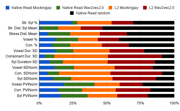
Native Read Speech: Figures 4(a2) and (b2)¹⁰¹⁰10Refer Tables 9 and 13 of Appendix for the loss values show the results for probing pronunciation features on wav2vec2.0 and Mockingjay with the Librispeech data. These features are learnt best by the last layers in Mockingjay. Wav2vec2.0 learns these features the most in the 6^th to 8^th layers amongst its $12$ layers. Mockingjay performs better for pronunciation-based features than wav2vec2.0 by $30.4\%$ in the final layer embeddings. Comparing the minimum loss layers for both models, the difference is $16.19\%$ in favor of Mockingjay.

Non-native Speech: Mockingjay follows the same pattern for L2 Arctic dataset as for the Librispeech dataset. It learns these features better in the last layers. However, for wav2vec2.0, the layers learning each of these pronunciation features are more spread out across the initial layers of the second half of the model. Wav2vec2.0 outperforms Mockingjay but the differences here are reduced to $8.9\%$ in the end layer and $2.20\%$ in the best performing layer. This pattern follows the non-native speech performance of wav2vec2.0 and Mockingjay seen with audio and fluency features. Here too, the performance difference between wav2vec2.0 and Mockingjay widens when compared to the native speech scenario.

4.4. Feature Extractor Module of wav2vec2.0

As shown in Figure 1, wav2vec2.0 has 7 convolutional layers before the transformer encoder block. The authors call it the “feature extractor” of wav2vec2.0. While in the computer vision community, it has been shown that subsequent layers of a CNN architecture look for higher level features, in the speech community this question has largely been left unaddressed (Erhan et al., 2010; Gong and Poellabauer, 2018). We find that there is a uniform increase in performance of the subsequent CNN layers for all feature types (audio, fluency, and pronunciation) and there is no difference between any features with respect to “high-level” or “low-level”. Figure 8 shows this behavior for audio features(which are supposed to be best learnt by feature extractor of audio transformer). The CNN layers faithfully extract all the features and show minimum loss at the seventh layer or the post-projection layers.

5. Can Audio Models Read Too?

Speech combines the text and the audio parts of the language. Conventionally, the audio community (which also deals with speech) has been more involved with signal sciences while the NLP community has dealt with the text part of speech while ignoring audio. This approach is suboptimal. However, due to the impressive performance of self-supervised transformers in every domain, there is a newfound interest in learning task-independent representations. Concurrently, there is also an interest in learning how these representations are working. Therefore, we probe to check whether the self-supervised audio transformers on account of their self-supervision tasks have accumulated some knowledge present in the text as well. With this motivation, we probe the audio transformer representations for surface (§5.1), syntax (§5.3) and semantic (§5.2) knowledge. For reference, we compare them with BERT based text-only embeddings. We use random embeddings as baseline. We do the experiments for four speech types (native read, native spontaneous, non-native, and artificial speech).

While the surface features measure the non-linguistic surface knowledge of the encoders, syntax features measure the syntax based linguistic properties. Conneau et al. (Conneau et al., 2018) include features such as sentence length and word content in surface features and syntax tree depth in syntax feature. The other category of features we measure are semantics features in which we include number of objects and subjects (Conneau et al., 2018).

Text feature	Description
Surface Features
Unique word count	Total count of unique words(Ignore words of length 3 or smaller)
Word Complexity	Sum of word complexities for all words in text given by annotators
Semantic Features
Total adjectives	Total count of adjectives
Total adverbs	Total count of adverbs
Total nouns	Total count of nouns
Total verbs	Total count of verbs
Total pronouns	Total count of pronouns
Total conjunction	Total count of conjunction
Total conjunction	Total count of conjunction
Number of subject	Total count of subject
Number of Object	Total count of direct objects
Tense	Classification of main clause verb into present or past tense
Syntax Feature
Depth of syntax tree	Depth of syntax tree of the text

Table 4. Text feature extraction algorithms extracted using nltk and numpy libraries

5.1. Surface Level Features

Surface level features measure the surface properties of sentences. No linguistic knowledge is required for these features. They can be measured by just looking at the tokens (Conneau et al., 2018). We include the following features - unique word count and the average word complexity (Word Complexity) since the lexical diversity of spoken speech is an important metric to evaluate its quality (Read et al., 2006).

Native Read Speech: When compared on LibriSpeech, surface-based features are learnt better by Mockingjay than wav2vec2.0 by $9.99\%$ and (b3)¹¹¹¹11Refer Tables LABEL:Vocab_W and 14 of Appendix for the loss values. These features are learnt best in the intermediate layers in wav2vec2.0 and initial layers in Mockingjay. From the results, we observe that the text understanding of both models becomes increasingly diffused as we go towards the later layers. However, wav2vec2.0 outperforms Mockingjay by $3.01\%$ in the final layer. A contributing factor to these observations is the learning of surface features by Mockingjay in the initial layers while, wav2vec2.0 learns it best in the middle layers.

Non-native Speech: For L2 arctic data, again wav2vec2.0 best learns the surface features in the middle layers but for mockingjay, no particular pattern is observed. The difference widens to $38.41\%$ on the end layers and $18.96\%$ on the minimum loss layer in favour of wav2vec2.0.

Native Spontaneous Speech:Mockingjay learns best in the initial layers like in the case with native read speech meanwhile, wav2vec2.0 performs best in the lower middle(7-11) layers. The difference increases to $141.42\%$ for native spontaneous speech on the final layer and $132.44\%$ on the best performing layer.

5.2. Semantic Level Features

The relationship between the words spoken and our comprehension of that spoken content falls into the domain of semantics. To produce meaning in a sentence, it is almost necessary for it to have a subject and a direct object that the subject addresses. The number of subjects, number of direct objects and total nouns, pronouns, adverbs, adjectives, verbs, conjunction, and determiners are hence in our set of features to evaluate the spoken content. (Conneau et al., 2018; Jawahar et al., 2019). We also probe for the tense(past or present) and it is framed as a classification task unlike the rest which are regression tasks so the result for tense are separately mentioned.

Native Read Speech: wav2vec2.0 performs better in this setting by $4.173\%$ and $5.29\%$ on the minimum loss layer. Like the surface features, the pattern followed by the layers in learning is same for semantic features. Mockingjay learns them best in initial layers while wav2vec2.0 in the intermediate layers. For tense too, wav2vec2.0 best performs with $75.04\%$ accuracy in the seventh layer where Mockingjay performs with $56.99\%$ in the last layer.

Non-native Speech:The same pattern as surface features in the non-native setting is followed by both the transformers. Mockingjay does not follow a clear pattern but wav2vec2.0 performs best in the middle layers. While wav2vec2.0 outperforms Mockingjay be $7.36\%$ on minimum layer loss for L2 speech, the margin decreases to $3.26\%$ on the end layer. Accuracy for tense is $57.95\%$ for wav2vec2.0 and $52.27\%$ for Mockingjay on 5th and 9th layer respectively.

Native Spontaneous Speech:Mockingjay does not concentrate its learning in any particular layer but wav2vec2.0 performs best in the second half of the transformer layers. wav2vec2.0 performs better by $9.83\%$ for native spontaneous speech on the best performing layer and $8.06\%$ on the final layer. Again for tense, the accuracy is $65.79\%$ on wav2vec2.0 and $57.89\%$ on Mockingjay.

5.3. Syntax Level Features

Syntax is the key component of the grammatical structure of a sentence, which in turn is a key component of the communicative competence (Canale and Swain, 1980). We use the depth of the syntax tree constructed from the sentences spoken in each sound clip as a feature to evaluate the syntax content (Conneau et al., 2018; Jawahar et al., 2019; Kumar et al., 2019).

Native Read Speech:In this setting as well, Mockingjay performs better than wav2vec2.0 by $38.64\%$ on the best performing layer and by $21.5\%$ on the final layer. The final layer captures this feature best for wav2vec2.0 and the initial for Mockingjay, which explains the decrease in percentage difference for the final layer.

Non-native Speech: wav2vec2.0 performs better on minimum layer loss by $15.89\%$ and $30.92\%$ on the final layer. wav2vec2.0 learns best on eight layer and Mockingjay learns best on fourth layer.

Native Spontaneous Speech:

5.4. Feature Extractor Module of wav2vec2.0

The pattern observed in the feature extractor module for these surface level features is the same as that of audio features with minimum losses seen in the post projection layer. However, the value of the minimum loss in this layer is less than that of the transformer module in wav2vec2.0. This gives some intuition for the better performance of Mockingjay since the Transformer is unable to capture the features or unlearns the presented vocabulary features.

5.5. Comparison with BERT

Dataset	Model	Semantic	Syntax	Surface
Native Read Speech	wav2vec2.0	-43.62%, -40.23%	-56.90%, -67.15%	-59.53%, -51.31%
	Mockingjay	-41.78%, -39.55%	-73.57%, -74.21%	-52.20%, -47.99%
Non-native Read Speech	wav2vec2.0	15.88%, 7.35%	59.05%, 30.33%	78.27%, -3.94%
	Mockingjay	24.30%, 11.14%	79.72%, 33.97%	121.71%, 21.30%
Wikipedia TTS	wav2vec2.0	10.22%, -2.29%	-34.55%, 3.83%	17.70%, -7.58%
	Mockingjay	13.87%, -0.49%	-47.70%, 7.68%	4.04%, 21.90%

Table 5. Table for comparison of the performance of BERT with wav2vec2.0 and Mockingjay on text features. The two values mentioned per cell indicate the relative minimum loss across all the model layers and the relative end layer losses when compared with the corresponding values for BERT. The values shown are an average across all features of a particular category with the relative performance calculated as

(model\_loss-bert\_loss)*100\%/bert\_loss

When we compare the performance of audio-transformer models with BERT (Table 5) on the native read speech, we observe that on an average, both wav2vec2.0 and Mockingjay perform better than BERT by 43.62% and 41.78% on semantic features, 56.90% and 73.57% on syntactic features and 59.53% and 52.20% on semantic features respectively. These results are surprising since none of the speech transformer models was trained with text objective functions. We hypothesize that this could be due to differences in the train set of the three models. LibriSpeech is the train-set for both the speech-transformer models where as Wikipedia is the train-set for BERT. To confirm this, we test the performance of the three models on text features extracted from Wikipedia and native spontaneous speech datasets. These datasets provide us with a comprehensive comparison. While on one hand, Wikipedia is the train-set for BERT, and the text features from Wikipedia articles are very different from LibriSpeech, on the other, non-native read speech dataset can be considered out-of-domain for both the speech transformer models and BERT.

For the first part, we convert 2000 random sentences from Wikipedia articles to speech by using Google’s text-to-speech API (Durette and Contributors, 2020). We made sure that the audios constructed had similar lengths as those of LibriSpeech. The audios obtained were then passed through both the speech Transformer models and the layers were then probed. On this synthetic dataset, for the semantic features, BERT outperforms both the models by more than 10% when compared on minimum loss across all the layers. However, by the end layers, both the models learn the features well and the performance difference between BERT and audio-transformer models reduces greatly ( $2.29\%$ and $0.49\%$ difference for semantic features, $3.83\%$ and $7.68\%$ for syntax and $7.58\%$ and $21.90\%$ for surface features). These results are motivating since this means that embeddings of audio Transformer captures not only audio, fluency and pronunciation features, but also textual features to a large extent.

Next, we use the CMU L2 Arctic dataset. Table 5 presents the results for all the experiments. Here the results are the most different from the previous ones. For the semantic, syntax and surface features, BERT outperforms both the models by more than $15\%$ . This result when compared with Wikipedia TTS and native read speech implies that the audio models capture text features for native speakers in ‘cleaner settings’ but they are not able to work in not-so controlled environments. Therefore, in a general setting, BERT text embeddings combined with audio embeddings can capture all the speech features adequately.

6. Effect on Downstream Tasks

We wanted to evaluate our findings which show that different layers of the models capture different features and see its impact on downstream tasks. To this end, we perform two representative tasks: speaker recognition on Voxceleb (Nagrani et al., 2017) (which uses audio features primarily), and phone classification on LibriSpeech (which uses pronunciation features).

For speaker recognition, we randomly pick $10$ speakers with $50$ audios each in the train-set and $10$ in the test-set. For phone classification, we use the libri-clean-100 and libri-cleanTest splits. We build a 4-layer linear classifier with dimensions $756,512,256,10$ with Adam optimizer and a learning rate of $0.01$ . Hidden layers have ReLU activation function and the third layer also has dropout. We perform the tasks using the best performing, final, and weighted average of all layer embeddings of the transformer models as input.

	Best	Last	Wtd Avg
wav2vec2.0	91%/81%	31%/70%	87%/77%
Mockingjay	10%/83%	32%/83%	26%/79%

Table 6. Comparison of the performance of wav2vec2.0 and Mockingjay on (speaker recognition/phone classification) tasks. Here best denotes best performing layer, i.e., first for audio features and sixth for pronunciation for wav2vec2.0.

Results for both the tasks are given in Table 6. The results are consistent with those found for audio (§4.1) and pronunciation features (§4.3).

7. Other Related Work

We already covered closely related work on attribution in Sections 1 and 2. We mention other related work.

Audio Probing: In the domain of speech processing, probes have been carried out on feature vectors, neural networks like RNN or DNN, end-to-end ASR systems or Audio-visual models. In (Raj et al., 2019), probing on x-vectors which are trained solely to predict the speaker label revealed they also contain incidental information about the transcription, channel, or meta-information about the utterance. Probing the Music Information Retrieval(MIR) prediction through Local Interpretable Model-Agnostic Explanations (LIME) by using AudioLIME (Haunschmid et al., 2020) helped interpret MIR for the first time. (Nagamine et al., 2015) analyses a DNN for phoneme recognition, both at single node and poplation level. Further research on interpretation of the role of non-linear activation of the nodes of a sigmoid DNN built for phoneme recognition task is done in (Nagamine et al., 2016). Research has also been done to address why LSTMs work well as a sequence model for statistical parametric speech synthesis (Wu and King, 2016). Several other studies have been conducted to interpret the correlation between audio and image structures for audio-visual tasks (Alishahi et al., 2017; Drexler and Glass, 2017; Harwath and Glass, 2017). Even for Deep ASR models, efforts have been made to comprehend the hidden and learned representations (Belinkov and Glass, 2017; Elloumi et al., 2018). However, probing of representation learning audio transformers is yet unexplored.

Text Probing: The field of natural language processing has seen numerous efforts in understanding the inner working of large-scale transformers, especially BERT (Jawahar et al., 2019; Cui et al., 2020; Ramnath et al., 2020). Jawahar et al. (2019) probe each of the different layers of BERT to find which layers best learn the phrase-level information, linguistic information and the long-distance dependencies. The results showed what role each layer played and the study concluded that the middle layers learnt the syntactic features and the higher levels learnt the semantic features and that the deeper layers are needed for long-distance dependencies while the initial layers capture the phrase-level information.

8. Conclusion

Speech transformer models, while still being new, have shown state-of-the-art performance on various downstream tasks. We probe two such models, wav2vec2.0 and Mockingjay, to understand what they learn. We probe the models on a wide range of features including audio, fluency, suprasegmental pronunciation, and text-based characteristics. For each category of features, we identify a learning pattern over each model and its layers. We find that wav2vec2.0 outperforms Mockingjay on audio and fluency features but underperforms on pronunciation features. Furthermore, we compare BERT with the audio models with text features and find that the audio models surprisingly outperform BERT in cleaner, controlled settings of native speech, but are not able to perform in an uncontrolled environment such as of spontaneous speech and non-native speech.

Acknowledgements.

To Robert, for the bagels and explaining CMYK and color spaces.

References

(1)
Alishahi et al. (2017) Afra Alishahi, Marie Barking, and Grzegorz Chrupała. 2017. Encoding of phonology in a recurrent neural model of grounded speech. In Proceedings of the 21st Conference on Computational Natural Language Learning (CoNLL 2017). 368–378.
Ardila et al. (2019) Rosana Ardila, Megan Branson, Kelly Davis, Michael Henretty, Michael Kohler, Josh Meyer, Reuben Morais, Lindsay Saunders, Francis M Tyers, and Gregor Weber. 2019. Common voice: A massively-multilingual speech corpus. arXiv preprint arXiv:1912.06670 (2019).
Baevski et al. (2019) Alexei Baevski, Steffen Schneider, and Michael Auli. 2019. vq-wav2vec: Self-Supervised Learning of Discrete Speech Representations. In International Conference on Learning Representations.
Baevski et al. (2020) Alexei Baevski, Henry Zhou, Abdelrahman Mohamed, and Michael Auli. 2020. wav2vec 2.0: A framework for self-supervised learning of speech representations. arXiv preprint arXiv:2006.11477 (2020).
Barth et al. (2014) Amy E Barth, Tammy D Tolar, Jack M Fletcher, and David Francis. 2014. The effects of student and text characteristics on the oral reading fluency of middle-grade students. Journal of Educational Psychology 106, 1 (2014), 162.
Belinkov et al. (2017) Yonatan Belinkov, Nadir Durrani, Fahim Dalvi, Hassan Sajjad, and James Glass. 2017. What do neural machine translation models learn about morphology? arXiv preprint arXiv:1704.03471 (2017).
Belinkov and Glass (2017) Yonatan Belinkov and James Glass. 2017. Analyzing hidden representations in end-to-end automatic speech recognition systems. In Advances in Neural Information Processing Systems. 2441–2451.
Boersma and Weenink (2021) Paul Boersma and David Weenink. 2021. Praat: doing phonetics by computer [Computer program]. Version 6.1.38, retrieved 2 January 2021 http://www.praat.org/.
Canale and Swain (1980) Michael Canale and Merrill Swain. 1980. Theoretical bases of communicative approaches to second language teaching and testing. Applied linguistics 1, 1 (1980), 1–47.
Chi et al. (2020) Po-Han Chi, Pei-Hung Chung, Tsung-Han Wu, Chun-Cheng Hsieh, Shang-Wen Li, and Hung-yi Lee. 2020. Audio ALBERT: A Lite BERT for Self-supervised Learning of Audio Representation. arXiv preprint arXiv:2005.08575 (2020).
Choi et al. (2017) Keunwoo Choi, György Fazekas, Kyunghyun Cho, and Mark Sandler. 2017. A tutorial on deep learning for music information retrieval. arXiv preprint arXiv:1709.04396 (2017).
Conneau et al. (2018) Alexis Conneau, Germán Kruszewski, Guillaume Lample, Loïc Barrault, and Marco Baroni. 2018. What you can cram into a single vector: Probing sentence embeddings for linguistic properties. arXiv preprint arXiv:1805.01070 (2018).
Cui et al. (2020) Leyang Cui, Sijie Cheng, Yu Wu, and Yue Zhang. 2020. Does BERT Solve Commonsense Task via Commonsense Knowledge? arXiv preprint arXiv:2008.03945 (2020).
De Jong and Wempe (2009) Nivja H De Jong and Ton Wempe. 2009. Praat script to detect syllable nuclei and measure speech rate automatically. Behavior research methods 41, 2 (2009), 385–390.
Derwing and Munro (1997) Tracey M Derwing and Murray J Munro. 1997. Accent, comprehensibility and intelligibility: Evidence from four L1s. Studies in Second Language Acquisition 19, 1 (1997), 1–16.
Devlin et al. (2019) Jacob Devlin, Ming-Wei Chang, Kenton Lee, and Kristina Toutanova. 2019. BERT: Pre-training of Deep Bidirectional Transformers for Language Understanding. In Proceedings of the 2019 Conference of the North American Chapter of the Association for Computational Linguistics: Human Language Technologies, Volume 1 (Long and Short Papers). Association for Computational Linguistics, Minneapolis, Minnesota, 4171–4186. https://doi.org/10.18653/v1/N19-1423
Doumbouya et al. (2021) Moussa Doumbouya, Lisa Einstein, and Chris Piech. 2021. Using Radio Archives for Low-Resource Speech Recognition: Towards an Intelligent Virtual Assistant for Illiterate Users. In Proceedings of the AAAI Conference on Artificial Intelligence, Vol. 35.
Drexler and Glass (2017) Jennifer Drexler and James Glass. 2017. Analysis of audio-visual features for unsupervised speech recognition. In Grounded Language Understanding Workshop.
Durette and Contributors (2020) Pierre Nicolas Durette and Contributors. 2020. Google Text to Speech Model. https://pypi.org/project/gTTS/.
Elloumi et al. (2018) Zied Elloumi, Laurent Besacier, Olivier Galibert, and Benjamin Lecouteux. 2018. Analyzing Learned Representations of a Deep ASR Performance Prediction Model. In Blackbox NLP Workshop and EMLP 2018.
Erhan et al. (2010) Dumitru Erhan, Aaron Courville, and Yoshua Bengio. 2010. Understanding representations learned in deep architectures. Department dInformatique et Recherche Operationnelle, University of Montreal, QC, Canada, Tech. Rep 1355, 1 (2010).
Garofolo et al. (1993) John S Garofolo, Lori F Lamel, William M Fisher, Jonathan G Fiscus, and David S Pallett. 1993. DARPA TIMIT acoustic-phonetic continous speech corpus CD-ROM. NIST speech disc 1-1.1. STIN 93 (1993), 27403.
Giannakopoulos (2015) Theodoros Giannakopoulos. 2015. pyaudioanalysis: An open-source python library for audio signal analysis. PloS one 10, 12 (2015), e0144610.
Girshick et al. (2014) Ross Girshick, Jeff Donahue, Trevor Darrell, and Jitendra Malik. 2014. Rich feature hierarchies for accurate object detection and semantic segmentation. In Proceedings of the IEEE conference on computer vision and pattern recognition. 580–587.
Gong and Poellabauer (2018) Yuan Gong and Christian Poellabauer. 2018. How do deep convolutional neural networks learn from raw audio waveforms? (2018).
Grover et al. (2020) Manraj Singh Grover, Yaman Kumar, Sumit Sarin, Payman Vafaee, Mika Hama, and Rajiv Ratn Shah. 2020. Multi-modal Automated Speech Scoring using Attention Fusion. arXiv preprint arXiv:2005.08182 (2020).
Harwath and Glass (2017) David Harwath and James Glass. 2017. Learning Word-Like Units from Joint Audio-Visual Analysis. In Proceedings of the 55th Annual Meeting of the Association for Computational Linguistics (Volume 1: Long Papers). 506–517.
Haunschmid et al. (2020) Verena Haunschmid, Ethan Manilow, and Gerhard Widmer. 2020. audioLIME: Listenable Explanations Using Source Separation. arXiv preprint arXiv:2008.00582 (2020).
Hewitt and Manning (2019) John Hewitt and Christopher D Manning. 2019. A structural probe for finding syntax in word representations. In Proceedings of the 2019 Conference of the North American Chapter of the Association for Computational Linguistics: Human Language Technologies, Volume 1 (Long and Short Papers). 4129–4138.
Igras-Cybulska et al. (2016) Magdalena Igras-Cybulska, Bartosz Ziółko, Piotr Żelasko, and Marcin Witkowski. 2016. Structure of pauses in speech in the context of speaker verification and classification of speech type. EURASIP Journal on Audio, Speech, and Music Processing 2016, 1 (2016), 18.
Jadoul et al. (2018) Yannick Jadoul, Bill Thompson, and Bart de Boer. 2018. Introducing Parselmouth: A Python interface to Praat. Journal of Phonetics 71 (2018), 1–15. https://doi.org/10.1016/j.wocn.2018.07.001
Jawahar et al. (2019) Ganesh Jawahar, Benoît Sagot, and Djamé Seddah. 2019. What Does BERT Learn about the Structure of Language?. In Proceedings of the 57th Annual Meeting of the Association for Computational Linguistics. Association for Computational Linguistics, Florence, Italy, 3651–3657. https://doi.org/10.18653/v1/P19-1356
Jyothi and Hasegawa-Johnson (2015) Preethi Jyothi and Mark Hasegawa-Johnson. 2015. Improved Hindi broadcast ASR by adapting the language model and pronunciation model using a priori syntactic and morphophonemic knowledge. In Sixteenth Annual Conference of the International Speech Communication Association.
Kitaev and Klein (2018) Nikita Kitaev and Dan Klein. 2018. Constituency parsing with a self-attentive encoder. arXiv preprint arXiv:1805.01052 (2018).
Krizhevsky et al. (2012) Alex Krizhevsky, Ilya Sutskever, and Geoffrey E Hinton. 2012. Imagenet classification with deep convolutional neural networks. Advances in neural information processing systems 25 (2012), 1097–1105.
Kumar et al. (2019) Yaman Kumar, Swati Aggarwal, Debanjan Mahata, Rajiv Ratn Shah, Ponnurangam Kumaraguru, and Roger Zimmermann. 2019. Get IT Scored Using AutoSAS—An Automated System for Scoring Short Answers. In Proceedings of the AAAI Conference on Artificial Intelligence, Vol. 33. 9662–9669.
Kyriakopoulos et al. (2020) Konstantinos Kyriakopoulos, Katherine Knill, and Mark Gales. 2020. Automatic detection of accent and lexical pronunciation errors in spontaneous non-native English speech. (2020).
Lee and Kim (2019) Younggun Lee and Taesu Kim. 2019. Robust and fine-grained prosody control of end-to-end speech synthesis. In ICASSP 2019-2019 IEEE International Conference on Acoustics, Speech and Signal Processing (ICASSP). IEEE, 5911–5915.
Liu et al. (2020) Andy T Liu, Shu-wen Yang, Po-Han Chi, Po-chun Hsu, and Hung-yi Lee. 2020. Mockingjay: Unsupervised speech representation learning with deep bidirectional transformer encoders. In ICASSP 2020-2020 IEEE International Conference on Acoustics, Speech and Signal Processing (ICASSP). IEEE, 6419–6423.
McFee et al. (2015) Brian McFee, Colin Raffel, Dawen Liang, Daniel PW Ellis, Matt McVicar, Eric Battenberg, and Oriol Nieto. 2015. librosa: Audio and music signal analysis in python. In Proceedings of the 14th python in science conference, Vol. 8. Citeseer, 18–25.
Möhle (1984) Dorothea Möhle. 1984. A comparison of the second language speech production of different native speakers. Second language productions 26 (1984), 49.
Mooney (2014) Ray Mooney. 2014. You can’t cram the meaning of a whole %&!$# sentence into a single $&!#* vector! https://www.cs.utexas.edu/~mooney/cramming.html.
Mulholland et al. (2016) Matthew Mulholland, Melissa Lopez, Keelan Evanini, Anastassia Loukina, and Yao Qian. 2016. A comparison of ASR and human errors for transcription of non-native spontaneous speech. In 2016 IEEE International Conference on Acoustics, Speech and Signal Processing (ICASSP). IEEE, 5855–5859.
Nagamine et al. (2015) Tasha Nagamine, Michael L Seltzer, and Nima Mesgarani. 2015. Exploring how deep neural networks form phonemic categories. In Sixteenth Annual Conference of the International Speech Communication Association.
Nagamine et al. (2016) Tasha Nagamine, Michael L Seltzer, and Nima Mesgarani. 2016. On the Role of Nonlinear Transformations in Deep Neural Network Acoustic Models.. In Interspeech. 803–807.
Nagrani et al. (2017) Arsha Nagrani, Joon Son Chung, and Andrew Zisserman. 2017. Voxceleb: a large-scale speaker identification dataset. arXiv preprint arXiv:1706.08612 (2017).
Neumayer and Rauber (2007) Robert Neumayer and Andreas Rauber. 2007. Integration of text and audio features for genre classification in music information retrieval. In European Conference on Information Retrieval. Springer, 724–727.
Panayotov et al. (2015) Vassil Panayotov, Guoguo Chen, Daniel Povey, and Sanjeev Khudanpur. 2015. Librispeech: an asr corpus based on public domain audio books. In 2015 IEEE International Conference on Acoustics, Speech and Signal Processing (ICASSP). IEEE, 5206–5210.
Patil et al. (2020) Rajaswa Patil, Yaman Kumar Singla, Rajiv Ratn Shah, Mika Hama, and Roger Zimmermann. 2020. Towards Modelling Coherence in Spoken Discourse. arXiv preprint arXiv:2101.00056 (2020).
Peters et al. (2018) Matthew E Peters, Mark Neumann, Mohit Iyyer, Matt Gardner, Christopher Clark, Kenton Lee, and Luke Zettlemoyer. 2018. Deep contextualized word representations. arXiv preprint arXiv:1802.05365 (2018).
Prasad and Jyothi (2020) Archiki Prasad and Preethi Jyothi. 2020. How Accents Confound: Probing for Accent Information in End-to-End Speech Recognition Systems. In Proceedings of the 58th Annual Meeting of the Association for Computational Linguistics. 3739–3753.
Raj et al. (2019) Desh Raj, David Snyder, Daniel Povey, and Sanjeev Khudanpur. 2019. Probing the information encoded in x-vectors. In 2019 IEEE Automatic Speech Recognition and Understanding Workshop (ASRU). IEEE, 726–733.
Ramnath et al. (2020) Sahana Ramnath, Preksha Nema, Deep Sahni, and Mitesh M Khapra. 2020. Towards Interpreting BERT for Reading Comprehension Based QA. arXiv preprint arXiv:2010.08983 (2020).
Rasinski (2004) Timothy V Rasinski. 2004. Assessing reading fluency. Pacific Resources for Education and Learning (PREL) (2004).
Read et al. (2006) John Read, Paul Nation, et al. 2006. An investigation of the lexical dimension of the IELTS speaking test. IELTS research reports 6 (2006), 207–231.
Simonetta et al. (2019) Federico Simonetta, Stavros Ntalampiras, and Federico Avanzini. 2019. Multimodal music information processing and retrieval: Survey and future challenges. In 2019 International Workshop on Multilayer Music Representation and Processing (MMRP). IEEE, 10–18.
Tang et al. (2020) Hao Tang, Donghong Ji, Chenliang Li, and Qiji Zhou. 2020. Dependency graph enhanced dual-transformer structure for aspect-based sentiment classification. In Proceedings of the 58th Annual Meeting of the Association for Computational Linguistics. 6578–6588.
Tian et al. (2020) Zhengkun Tian, Jiangyan Yi, Ye Bai, Jianhua Tao, Shuai Zhang, and Zhengqi Wen. 2020. Synchronous transformers for end-to-end speech recognition. In ICASSP 2020-2020 IEEE International Conference on Acoustics, Speech and Signal Processing (ICASSP). IEEE, 7884–7888.
Vaswani et al. (2017) Ashish Vaswani, Noam Shazeer, Niki Parmar, Jakob Uszkoreit, Llion Jones, Aidan N Gomez, Łukasz Kaiser, and Illia Polosukhin. 2017. Attention is all you need. In Advances in neural information processing systems. 5998–6008.
Wood (2001) David Wood. 2001. In search of fluency: What is it and how can we teach it? Canadian Modern Language Review 57, 4 (2001), 573–589.
Wu et al. (2020) Anne Wu, Changhan Wang, Juan Pino, and Jiatao Gu. 2020. Self-supervised representations improve end-to-end speech translation. arXiv preprint arXiv:2006.12124 (2020).
Wu and King (2016) Zhizheng Wu and Simon King. 2016. Investigating gated recurrent networks for speech synthesis. In 2016 IEEE International Conference on Acoustics, Speech and Signal Processing (ICASSP). IEEE, 5140–5144.
Yan et al. (2018) Xun Yan, Ha Ram Kim, and J Kim. 2018. Complexity, Accuracy and Fluency (CAF). Features of speaking performances on APTIS across different levels on the common European framework of reference for languages (CEFR).
Zhang et al. (2020) Xikun Zhang, Deepak Ramachandran, Ian Tenney, Yanai Elazar, and Dan Roth. 2020. Do Language Embeddings Capture Scales? arXiv preprint arXiv:2010.05345 (2020).
Zhang and Duan (2018) Yichi Zhang and Zhiyao Duan. 2018. Visualization and interpretation of Siamese style convolutional neural networks for sound search by vocal imitation. In 2018 IEEE International Conference on Acoustics, Speech and Signal Processing (ICASSP). IEEE, 2406–2410.
Zhang et al. (2019) Yu Zhang, Ron J Weiss, Heiga Zen, Yonghui Wu, Zhifeng Chen, RJ Skerry-Ryan, Ye Jia, Andrew Rosenberg, and Bhuvana Ramabhadran. 2019. Learning to speak fluently in a foreign language: Multilingual speech synthesis and cross-language voice cloning. arXiv preprint arXiv:1907.04448 (2019).
Zhao et al. (2018) Guanlong Zhao, Sinem Sonsaat, Alif Silpachai, Ivana Lucic, Evgeny Chukharev-Hudilainen, John Levis, and Ricardo Gutierrez-Osuna. 2018. L2-ARCTIC: A Non-native English Speech Corpus. In Proc. Interspeech. 2783–2787. https://doi.org/10.21437/Interspeech.2018-1110

Appendix A Experimental results

Features\Layers 1 2 3 4 5 6 7 8 9 10 11 12 Duration 0.001001 0.001053 0.001099 0.000988 0.000893 0.001037 0.000985 0.001205 0.001173 0.001198 0.001597 0.001742 stdev_energy 0.002307 0.00238 0.002714 0.003584 0.004343 0.004559 0.004829 0.004668 0.004243 0.003856 0.004065 0.004143 mean_pitch 0.001812 0.001821 0.002083 0.00279 0.003374 0.003993 0.003758 0.00421 0.003715 0.002609 0.003511 0.003896 voiced_to_unvoiced_ratio 0.002232 0.002014 0.001971 0.002092 0.00225 0.002457 0.00244 0.002375 0.00236 0.001863 0.002477 0.002677 zero_crossing_rate 0.0044 0.004152 0.004536 0.005638 0.006737 0.007006 0.008681 0.007473 0.006309 0.006546 0.007058 0.007533 energy_entropy 0.004003 0.003852 0.004065 0.004144 0.004913 0.004166 0.004566 0.00414 0.0042 0.004021 0.004928 0.005935 spectral_centroid 0.000335 0.000335 0.000335 0.000335 0.000335 0.000335 0.000335 0.000335 0.000335 0.000335 0.000335 0.000335 localJitter 0.002261 0.001933 0.002131 0.002111 0.002273 0.002446 0.002638 0.002834 0.002379 0.001996 0.002267 0.002489 localShimmer 0.003059 0.003057 0.003449 0.003517 0.004047 0.004389 0.004901 0.004478 0.004077 0.00355 0.004037 0.00396

Table 7. Results (MSE) for audio features on wav2vec2.0 for native read speech corpus (Librispeech)

Features\Layers 1 2 3 4 5 6 7 8 9 10 11 12 filled_pause_rate 0.000877 0.00093 0.00083 0.000917 0.000831 0.000838 0.00081 0.000782 0.000794 0.000802 0.000815 0.000829 general_silence 0.001896 0.001805 0.00194 0.001795 0.001684 0.001924 0.002031 0.001937 0.00198 0.002098 0.002722 0.002112 mean_silence 0.001807 0.001908 0.001891 0.001959 0.001821 0.001723 0.001787 0.001845 0.001906 0.001886 0.002394 0.002328 silence_abs_deviation 0.000975 0.001266 0.00149 0.001221 0.001371 0.001316 0.00158 0.001618 0.001493 0.001484 0.001869 0.001599 SilenceRate1 0.005096 0.004997 0.005074 0.004758 0.004217 0.003676 0.003839 0.004035 0.004023 0.00436 0.004927 0.005627 SilenceRate2 0.00516 0.00552 0.005248 0.004933 0.005085 0.004941 0.004845 0.005112 0.005174 0.00574 0.005895 0.006605 speaking_rate 0.013043 0.012784 0.012493 0.010239 0.007733 0.006184 0.005216 0.005029 0.005487 0.006623 0.009679 0.01164 articulation_rate 0.016824 0.015866 0.014793 0.012394 0.008917 0.007374 0.006135 0.006321 0.006001 0.007958 0.010589 0.011723 longpfreq 0.001642 0.001979 0.001774 0.001982 0.001731 0.001646 0.001798 0.001868 0.001698 0.001848 0.001863 0.001995 average_syllables_in_words 0.018313 0.018215 0.018016 0.015562 0.01167 0.008615 0.006652 0.006486 0.007123 0.010458 0.013834 0.014869 wordsyll2 0.010109 0.010726 0.011357 0.009438 0.007506 0.006293 0.005058 0.005559 0.005261 0.005988 0.008059 0.007614 repetition_freq 0.015586 0.016036 0.017251 0.016137 0.015412 0.014447 0.013344 0.01352 0.013318 0.015553 0.014703 0.013719

Table 8. Results (MSE) for fluency features on wav2vec2.0 for native read speech corpus (Librispeech)

Features\Layers 1 2 3 4 5 6 7 8 9 10 11 12 StressedSyllPercent 0.018905 0.019561 0.020112 0.018046 0.020365 0.002052 0.001923 0.001946 0.001741 0.002095 0.002429 0.002547 StressDistanceSyllMean 0.00951 0.009831 0.009026 0.00883 0.008503 0.008189 0.007759 0.007837 0.008494 0.00752 0.00922 0.008768 StressDistanceMean 0.01204 0.012537 0.012932 0.013452 0.01043 0.010614 0.011099 0.010778 0.010512 0.011903 0.011996 0.011983 vowelPercentage 0.007322 0.007084 0.006278 0.005989 0.005836 0.005385 0.005205 0.005008 0.004806 0.00545 0.006394 0.006526 consonantPercentage 0.00597 0.006529 0.007062 0.005323 0.005464 0.004765 0.004961 0.005012 0.004824 0.004472 0.005979 0.006222 vowelDurationSD 0.002792 0.002813 0.002516 0.002353 0.002159 0.002076 0.001875 0.001894 0.001866 0.001997 0.002379 0.002423 consonantDurationSD 0.001645 0.001361 0.001378 0.001352 0.001319 0.001274 0.001254 0.001392 0.001346 0.001282 0.001411 0.00154 syllableDurationSD 0.005843 0.005444 0.005413 0.004813 0.004507 0.003987 0.003908 0.003954 0.004033 0.004483 0.005114 0.005243 vowelSDNorm 0.003604 0.003876 0.003826 0.003511 0.003458 0.003277 0.003311 0.003346 0.00323 0.003449 0.003971 0.003586 consonantSDNorm 0.002454 0.002599 0.002593 0.002414 0.002399 0.0023 0.002272 0.002299 0.002389 0.002296 0.00252 0.00247 syllableSDNorm 0.006879 0.006955 0.007364 0.006514 0.00589 0.005689 0.005543 0.005619 0.005713 0.006977 0.007221 0.007269 vowelPVINorm 0.008083 0.008477 0.008793 0.00854 0.007294 0.007872 0.00736 0.008043 0.007457 0.008197 0.008581 0.008054 consonantPVINorm 0.007041 0.007458 0.007528 0.006909 0.006419 0.006852 0.006777 0.006805 0.007341 0.006959 0.007225 0.007434 syllablePVINorm 0.012702 0.013669 0.013096 0.012062 0.012077 0.011151 0.011088 0.011425 0.011091 0.01258 0.013119 0.013045

Table 9. Results (MSE) for pronunciation features on wav2vec2.0 for native read speech corpus (Librispeech)

Features\Layers 1 2 3 4 5 6 7 8 9 10 11 12 Unique Word count 0.005403 0.004279 0.006434 0.007045 0.004074 0.005392 0.004464 0.004928 0.007097 0.005556 0.005561 0.005696 Word Complexity 0.011001 0.010729 0.010597 0.010257 0.009527 0.009294 0.00883 0.009122 0.009118 0.009888 0.010307 0.010515 Total adjectives 0.008716 0.008636 0.008345 0.009197 0.009202 0.009062 0.007672 0.008421 0.007952 0.009323 0.009411 0.009366 Total adverbs 0.011648 0.011361 0.01115 0.010896 0.009901 0.00901 0.008756 0.00871 0.009569 0.010773 0.010703 0.01076 Total nouns 0.004879 0.005831 0.005286 0.004014 0.004326 0.004439 0.004539 0.004013 0.00385 0.004392 0.004874 0.005444 Total verbs 0.009748 0.008873 0.009065 0.008777 0.007376 0.006792 0.00808 0.007944 0.007044 0.009047 0.009181 0.008955 Total pronoun 0.002278 0.002251 0.00228 0.002274 0.002318 0.0021 0.002364 0.002101 0.001889 0.002211 0.00224 0.002304 Total conjunction 0.004891 0.004882 0.005034 0.004929 0.004822 0.004451 0.004238 0.004201 0.004505 0.00487 0.004885 0.004949 Total determiners 0.001954 0.001966 0.001957 0.00193 0.001954 0.002219 0.00232 0.001854 0.001931 0.001946 0.001956 0.001953 No. of subj 0.014399 0.016879 0.01675 0.016729 0.016072 0.014606 0.01289 0.015839 0.013978 0.013527 0.015682 0.013509 No. of obj 0.017454 0.01987 0.022306 0.021348 0.02231 0.022954 0.018353 0.020034 0.019796 0.018132 0.017848 0.016293 Tree depth 0.010957 0.01198 0.013783 0.01487 0.013179 0.017128 0.011726 0.016646 0.012092 0.011978 0.012764 0.009952

Table 10. Results (MSE) for text features on wav2vec2.0 for native read speech corpus (Librispeech)

Features\Layers 1 2 3 4 5 6 7 8 9 10 11 12 total_duration 0.0006 0.001195 0.002857 0.003293 0.003334 0.003413 0.003017 0.004304 0.003943 0.005397 0.005148 0.005897 stdev_energy 0.007231 0.005821 0.008878 0.00692 0.006879 0.006747 0.006156 0.00652 0.005613 0.005844 0.005424 0.005705 mean_pitch 0.002864 0.005313 0.009793 0.010587 0.009883 0.010169 0.009742 0.005038 0.003443 0.001832 0.000927 0.001272 voiced_to_unvoiced_ratio 0.004341 0.003959 0.005517 0.005531 0.005119 0.005269 0.006042 0.004361 0.002816 0.002329 0.002053 0.001834 zero_crossing_rate 0.011892 0.013714 0.014845 0.015256 0.01248 0.013971 0.012568 0.013016 0.011436 0.007881 0.008748 0.009278 energy_entropy 0.005736 0.005621 0.006332 0.006845 0.006357 0.006518 0.006331 0.006071 0.005919 0.00635 0.00684 0.00662 spectral_centroid 0.000335 0.000335 0.000335 0.000335 0.000335 0.000335 0.000335 0.000336 0.000348 0.000335 0.000335 0.000335 localJitter 0.002802 0.002952 0.003129 0.003784 0.003684 0.003827 0.003192 0.0031 0.002831 0.002181 0.002076 0.001966 localShimmer 0.006434 0.006935 0.007138 0.007962 0.0072 0.007752 0.007866 0.007677 0.006455 0.005965 0.005424 0.005135

Table 11. Results (MSE) for audio features on Mockingjay for native read speech corpus (Librispeech)

Features\Layers 1 2 3 4 5 6 7 8 9 10 11 12 filled_pause_rate 0.00079 0.000775 0.000776 0.000774 0.000773 0.000769 0.000775 0.00078 0.000785 0.000835 0.000815 0.000789 general_silence 0.003559 0.003244 0.002682 0.003353 0.003067 0.002264 0.002346 0.002401 0.003544 0.004336 0.004376 0.0046 mean_silence 0.002124 0.002661 0.002411 0.002158 0.001764 0.002073 0.001833 0.002313 0.001883 0.003345 0.001942 0.00174 silence_absolute_deviation 0.003095 0.002299 0.001743 0.001615 0.001543 0.001675 0.001372 0.002061 0.001954 0.00175 0.001509 0.002432 SilenceRate1 0.005183 0.005171 0.005297 0.005822 0.005221 0.005045 0.005098 0.004941 0.004533 0.004755 0.004788 0.004162 SilenceRate2 0.005451 0.004879 0.005217 0.005187 0.005731 0.005497 0.005417 0.004746 0.005169 0.005023 0.006062 0.006018 speaking_rate 0.012803 0.012767 0.014038 0.014252 0.014247 0.014811 0.013957 0.015266 0.012086 0.01259 0.011059 0.011137 articulation_rate 0.016709 0.016736 0.018223 0.018936 0.018751 0.018269 0.017996 0.019456 0.015512 0.014811 0.012795 0.013218 longpfreq 0.001566 0.001713 0.001707 0.001574 0.001661 0.001604 0.001672 0.001607 0.001571 0.001813 0.002025 0.0018 average_syllables_in_words 0.014321 0.013737 0.01423 0.015298 0.015195 0.014701 0.01449 0.014178 0.014282 0.015107 0.015409 0.014309 wordsyll2 0.010012 0.010246 0.012442 0.012758 0.011834 0.011637 0.011688 0.011879 0.011029 0.012438 0.012399 0.011999 repetition_freq 0.011282 0.011277 0.011447 0.011672 0.011502 0.011495 0.011444 0.011428 0.011734 0.01204 0.012926 0.012278

Table 12. Results (MSE) for fluency features on Mockingjay for native read speech corpus (Librispeech)

Features\Layers 1 2 3 4 5 6 7 8 9 10 11 12 StressedSyllPercent 0.016776 0.016777 0.017137 0.017021 0.01676 0.017471 0.016636 0.016884 0.016915 0.015961 0.016951 0.01643 StressDistanceSyllMean 0.002738 0.00502 0.008836 0.011745 0.009905 0.009778 0.009395 0.004853 0.003612 0.001711 0.00096 0.000799 StressDistanceMean 0.010448 0.011868 0.014704 0.016046 0.015573 0.015609 0.014304 0.011836 0.010375 0.007646 0.005007 0.004817 vowelPercentage 0.006115 0.006363 0.007021 0.007937 0.007496 0.007167 0.006866 0.005513 0.005456 0.004813 0.004648 0.004672 consonantPercentage 0.005199 0.005549 0.006474 0.00614 0.005955 0.005665 0.005455 0.005207 0.005086 0.004534 0.004377 0.004635 vowelDurationSD 0.002703 0.002683 0.002921 0.00286 0.003081 0.002907 0.002783 0.002688 0.002457 0.002194 0.002132 0.002288 consonantDurationSD 0.001128 0.001202 0.001373 0.001322 0.001312 0.001375 0.001264 0.001207 0.001089 0.001026 0.001074 0.000959 syllableDurationSD 0.004989 0.005503 0.005784 0.005818 0.005728 0.005975 0.005904 0.005596 0.004834 0.004513 0.004304 0.004305 vowelSDNorm 0.003146 0.002863 0.002959 0.002969 0.00301 0.002889 0.002947 0.002857 0.002926 0.002932 0.002937 0.00288 consonantSDNorm 0.001863 0.002026 0.001836 0.001915 0.001888 0.001876 0.001865 0.001871 0.001939 0.001928 0.001948 0.001851 syllableSDNorm 0.005986 0.005941 0.005994 0.005847 0.005853 0.005905 0.006004 0.005834 0.005789 0.005879 0.005828 0.005727 vowelPVINorm 0.006571 0.006466 0.006616 0.006877 0.006913 0.006888 0.006579 0.006727 0.006548 0.006447 0.006748 0.006356 consonantPVINorm 0.00558 0.005594 0.005786 0.005957 0.005809 0.005824 0.005664 0.005537 0.005373 0.005287 0.005391 0.005677 syllablePVINorm 0.010683 0.010746 0.011027 0.01068 0.010567 0.010839 0.0108 0.010717 0.010553 0.010659 0.011023 0.010602

Table 13. Results (MSE) for pronunciation features on Mockingjay for native read speech corpus (Librispeech)

Features\Layers 1 2 3 4 5 6 7 8 9 10 11 12 Unique Word count 0.002199 0.005996 0.00673 0.005919 0.006723 0.007532 0.005243 0.005413 0.006635 0.008469 0.011627 0.005578 Word Complexity 0.011128 0.011406 0.011535 0.011591 0.01167 0.011325 0.011527 0.01143 0.011467 0.012014 0.011469 0.011363 Total adjectives 0.00757 0.00882 0.009862 0.011036 0.010323 0.011291 0.009432 0.009538 0.010743 0.011471 0.012513 0.010343 Total adverbs 0.010991 0.011332 0.011315 0.011537 0.011498 0.011458 0.011387 0.011352 0.011593 0.012657 0.013342 0.01247 Total nouns 0.004011 0.004433 0.006881 0.007137 0.006792 0.006114 0.005585 0.006673 0.007262 0.007768 0.008683 0.006561 Total verbs 0.008358 0.009059 0.010349 0.010684 0.010196 0.01044 0.009787 0.009147 0.012781 0.013148 0.014656 0.011548 Total pronoun 0.002238 0.002217 0.00221 0.002231 0.002242 0.002281 0.002264 0.002303 0.002259 0.002374 0.002525 0.002345 Total conjunction 0.004935 0.004902 0.004965 0.005017 0.005184 0.00505 0.004963 0.005009 0.005076 0.00517 0.00555 0.005081 Total determiners 0.00194 0.001974 0.001944 0.001952 0.001968 0.001977 0.001941 0.001942 0.001977 0.002006 0.002023 0.001973 No. of subj 0.010997 0.010014 0.010586 0.011605 0.010631 0.011095 0.01074 0.010356 0.010707 0.011335 0.011679 0.011205 No. of obj 0.011757 0.011308 0.012495 0.012662 0.012242 0.012031 0.012256 0.012449 0.011985 0.01295 0.013274 0.013587 Tree depth 0.00611 0.006107 0.007302 0.011605 0.008775 0.007191 0.007097 0.00715 0.006802 0.007231 0.007594 0.007813

Table 14. Results (MSE) for text features on Mockingjay for native read speech corpus (Librispeech)

Features\Layers 1 2 3 4 5 6 7 8 9 10 11 12 total_duration 0.003037 0.002241 0.002387 0.002949 0.002987 0.002997 0.002993 0.00398 0.003188 0.003082 0.00443 0.005753 stdev_energy 0.013247 0.010778 0.013224 0.011689 0.011251 0.011181 0.011164 0.01123 0.012513 0.011796 0.011889 0.011455 mean_pitch 0.004493 0.003569 0.003843 0.004897 0.005505 0.004684 0.005197 0.005699 0.005733 0.004194 0.008189 0.006506 voiced_to_unvoiced_ratio 0.002074 0.002024 0.001661 0.002073 0.002288 0.001632 0.001988 0.001961 0.001982 0.001904 0.002233 0.002125 zero_crossing_rate 0.010519 0.007792 0.006901 0.007062 0.008208 0.00679 0.00718 0.006587 0.006429 0.006369 0.010559 0.009979 energy_entropy 0.013166 0.010519 0.008692 0.01036 0.010414 0.01094 0.010786 0.010152 0.013525 0.009774 0.010588 0.011592 spectral_centroid 0.000004 0.000003 0.000003 0.000003 0.000003 0.000003 0.000003 0.000004 0.000004 0.000003 0.000003 0.000003 localJitter 0.008843 0.00763 0.010089 0.007924 0.007034 0.008899 0.007446 0.01006 0.008025 0.007731 0.008643 0.008794 localShimmer 0.005666 0.00494 0.005273 0.004515 0.006485 0.004504 0.004659 0.005153 0.004648 0.005181 0.006095 0.005419

Table 15. Results (MSE) for audio features on wav2vec2.0 for non-native read speech corpus (L2 Arctic)

Features\Layers 1 2 3 4 5 6 7 8 9 10 11 12 filled_pause_rate 0.0000064 0.0000087 0.0000047 0.0000042 0.0000092 0.0000036 0.0000056 0.0000265 0.0000234 0.0000037 0.0000034 0.0000037 general_silence 0.010336 0.009149 0.009781 0.009449 0.010214 0.009557 0.010462 0.01013 0.009626 0.0107 0.00914 0.010858 mean_silence 0.008367 0.00818 0.008529 0.007218 0.007962 0.008569 0.007368 0.008397 0.00864 0.008453 0.009267 0.00882 silence_abs_deviation 0.008834 0.008651 0.008101 0.008431 0.008082 0.008105 0.008496 0.007868 0.007671 0.008466 0.009121 0.010871 SilenceRate1 0.010441 0.009092 0.010433 0.009222 0.009357 0.008964 0.009186 0.009738 0.010078 0.00949 0.008925 0.010444 SilenceRate2 0.019169 0.017716 0.01913 0.018713 0.018604 0.017923 0.018491 0.019281 0.018252 0.018755 0.017999 0.022653 speaking_rate 0.009495 0.008707 0.00915 0.009289 0.009674 0.008421 0.007933 0.008018 0.007882 0.009373 0.010031 0.009356 articulation_rate 0.014608 0.012277 0.011997 0.012936 0.012124 0.011002 0.011027 0.011786 0.01273 0.011808 0.012298 0.012386 longpfreq 0.006085 0.00566 0.00515 0.00531 0.004731 0.005081 0.005215 0.005338 0.005203 0.004949 0.005599 0.005909 average_syllables_in_words 0.040541 0.039341 0.038896 0.040124 0.034919 0.032039 0.026923 0.0319 0.030701 0.034601 0.046442 0.040721 wordsyll2 0.02971 0.029581 0.029094 0.027793 0.027336 0.026798 0.02158 0.023803 0.025616 0.02566 0.030421 0.028458 repetition_freq 0.025743 0.026271 0.026023 0.026202 0.026274 0.025517 0.025752 0.027057 0.026717 0.025908 0.026287 0.026288

Table 16. Results (MSE) for fluency features on wav2vec2.0 for non-native read speech corpus (L2 Arctic)

Features\Layers 1 2 3 4 5 6 7 8 9 10 11 12 StressDistanceSyllMean 0.010858 0.010986 0.011084 0.010706 0.010447 0.010925 0.01058 0.010629 0.010961 0.010965 0.010822 0.010862 StressDistanceMean 0.01445 0.01437 0.014744 0.014552 0.014447 0.014385 0.013805 0.014652 0.014157 0.014463 0.014664 0.014562 vowelPercentage 0.006582 0.006036 0.005799 0.005019 0.004906 0.005743 0.005376 0.005848 0.004815 0.005328 0.006171 0.006102 consonantPercentage 0.010776 0.009302 0.009351 0.011724 0.007659 0.006691 0.008678 0.008015 0.008811 0.008519 0.009191 0.009436 vowelDurationSD 0.004968 0.005062 0.004467 0.004498 0.004241 0.004157 0.00432 0.004319 0.004306 0.004624 0.004953 0.004792 consonantDurationSD 0.008937 0.008598 0.008309 0.008176 0.008196 0.007876 0.008254 0.008291 0.008224 0.00824 0.009342 0.008896 syllableDurationSD 0.018064 0.017007 0.016705 0.015943 0.016991 0.015742 0.015609 0.016092 0.016 0.016202 0.017674 0.019068 vowelSDNorm 0.00729 0.007269 0.007573 0.007196 0.007126 0.007205 0.00711 0.007452 0.007106 0.007388 0.007281 0.007137 consonantSDNorm 0.011117 0.010125 0.010393 0.010053 0.010329 0.01008 0.010348 0.010509 0.010004 0.011252 0.011404 0.011133 syllableSDNorm 0.015935 0.016013 0.015636 0.015655 0.017318 0.01532 0.014836 0.016397 0.017799 0.015735 0.01658 0.017679 vowelPVINorm 0.006011 0.006213 0.006066 0.006023 0.005908 0.005946 0.0058 0.005853 0.005862 0.00597 0.00606 0.005956 consonantPVINorm 0.009807 0.009825 0.010233 0.010364 0.010156 0.01187 0.009982 0.010278 0.01084 0.011683 0.010663 0.010516 syllablePVINorm 0.015131 0.014699 0.014601 0.014249 0.015095 0.015608 0.01386 0.015136 0.014716 0.01435 0.015585 0.014903

Table 17. Results (MSE) for pronunciation features on wav2vec2.0 for non-native read speech corpus (L2 Arctic)

Features\Layers 1 2 3 4 5 6 7 8 9 10 11 12 Unique Word count 0.016328 0.015269 0.01443 0.014206 0.016187 0.016495 0.013196 0.01333 0.014827 0.015252 0.016198 0.018124 Word Complexity 0.02358 0.025074 0.026571 0.023607 0.023869 0.022757 0.024556 0.023255 0.024087 0.02473 0.025855 0.026026 Total adjectives 0.055104 0.055733 0.055438 0.0582 0.053788 0.053288 0.051659 0.051016 0.055142 0.05502 0.058229 0.058659 Total adverbs 0.032355 0.031032 0.030508 0.031414 0.034148 0.03062 0.033625 0.031246 0.032231 0.0325 0.030786 0.030738 Total nouns 0.031529 0.032214 0.034053 0.032932 0.032949 0.029525 0.028352 0.029281 0.029507 0.030491 0.032188 0.033265 Total verbs 0.038064 0.037304 0.041601 0.037693 0.03675 0.040773 0.035506 0.037434 0.045298 0.040241 0.037563 0.037659 Total pronoun 0.019591 0.019544 0.01956 0.019596 0.019562 0.019445 0.019699 0.019446 0.019506 0.019491 0.019485 0.019494 Total conjunction 0.042578 0.042498 0.042017 0.041322 0.042358 0.042192 0.041659 0.041382 0.041127 0.041878 0.042459 0.042781 Total determiners 0.01978 0.019613 0.019911 0.01972 0.019727 0.019582 0.019646 0.019535 0.01958 0.019619 0.01961 0.019776 No. of subj 0.067824 0.065793 0.065282 0.066421 0.064326 0.065557 0.061022 0.061545 0.064313 0.065425 0.067203 0.068783 No. of obj 0.04038 0.040672 0.040469 0.041629 0.040958 0.039576 0.037172 0.036589 0.038272 0.040714 0.040737 0.042256 Tree depth 0.021626 0.021995 0.02262 0.022675 0.022558 0.021697 0.020467 0.021307 0.024375 0.023414 0.022422 0.023464

Table 18. Results (MSE) for text features on wav2vec2.0 for non-native read speech corpus (L2 Arctic)

Features\Layers 1 2 3 4 5 6 7 8 9 10 11 12 total_duration 0.011324 0.003763 0.007239 0.005672 0.005221 0.007031 0.007505 0.007055 0.007161 0.007567 0.010025 0.012677 stdev_energy 0.015313 0.015339 0.016494 0.014493 0.01403 0.015362 0.013972 0.017967 0.014863 0.013474 0.011171 0.012512 mean_pitch 0.016319 0.017864 0.013842 0.014276 0.011206 0.0148 0.017934 0.011364 0.008506 0.003965 0.003368 0.003793 voiced_to_unvoiced_ratio 0.002841 0.002697 0.002844 0.002684 0.002754 0.002926 0.00292 0.002638 0.002202 0.001792 0.00161 0.002214 zero_crossing_rate 0.011983 0.013096 0.011805 0.012052 0.011352 0.013772 0.017485 0.012387 0.007931 0.007328 0.004908 0.005565 energy_entropy 0.014261 0.013957 0.011386 0.011758 0.013304 0.012495 0.015632 0.014125 0.016826 0.012122 0.013926 0.015025 spectral_centroid 0.000003 0.000003 0.000003 0.000003 0.000004 0.000003 0.000005 0.000003 0.000003 0.000003 0.000003 0.000005 localJitter 0.009555 0.009915 0.008388 0.009049 0.00897 0.011487 0.011618 0.007706 0.007508 0.007772 0.007588 0.007487 localShimmer 0.007763 0.007366 0.0061 0.006087 0.006472 0.006134 0.007093 0.00579 0.006633 0.005442 0.006895 0.004808

Table 19. Results (MSE) for audio features on Mockingjay for non-native read speech corpus (L2 Arctic)

Features\Layers 1 2 3 4 5 6 7 8 9 10 11 12 filled_pause_rate 0.0000015 0.0000054 0.0000017 0.0000085 0.0000039 0.0000132 0.0000001 0.0000134 0.0000775 0.0000016 0.0000036 0.0000513 general_silence 0.013079 0.011675 0.011336 0.010921 0.010777 0.010924 0.012546 0.011623 0.01091 0.009547 0.011005 0.012333 mean_silence 0.009038 0.008802 0.00913 0.009513 0.010127 0.011607 0.010981 0.008231 0.007322 0.008047 0.007277 0.007887 silence_abs_deviation 0.008988 0.007935 0.009433 0.009917 0.008996 0.009184 0.009437 0.008632 0.007513 0.00863 0.008548 0.009037 SilenceRate1 0.011366 0.0108 0.011012 0.009303 0.009495 0.010584 0.009934 0.009442 0.009309 0.0089 0.008661 0.009029 SilenceRate2 0.020763 0.019909 0.019526 0.018436 0.021103 0.018528 0.019417 0.018365 0.017279 0.017109 0.01662 0.018189 speaking_rate 0.010575 0.010034 0.009617 0.009627 0.009733 0.010429 0.013854 0.01039 0.010063 0.011578 0.010152 0.009589 articulation_rate 0.015664 0.014572 0.015364 0.014105 0.013773 0.015194 0.017737 0.016386 0.015303 0.01375 0.013596 0.015014 longpfreq 0.007634 0.006734 0.009045 0.006316 0.005609 0.006313 0.006256 0.005071 0.004951 0.004762 0.004741 0.004901 average_syllables_in_words 0.047811 0.053749 0.041714 0.043455 0.044667 0.047274 0.043626 0.044136 0.043008 0.04317 0.043801 0.045771 wordsyll2 0.037088 0.03632 0.035302 0.034771 0.037232 0.038009 0.036853 0.037443 0.03709 0.035578 0.036575 0.035855 repetition_freq 0.02641 0.026258 0.026411 0.026243 0.026179 0.026339 0.02649 0.026482 0.026486 0.026519 0.026192 0.026305

Table 20. Results (MSE) for fluency features on Mockingjay for non-native read speech corpus (L2 Arctic)

Features\Layers 1 2 3 4 5 6 7 8 9 10 11 12 StressDistanceSyllMean 0.0110454 0.011099 0.0113248 0.0108703 0.0109954 0.0108252 0.0109959 0.0110083 0.0110286 0.0111566 0.0108324 0.0112061 StressDistanceMean 0.015089 0.015405 0.014999 0.015803 0.014757 0.015073 0.015133 0.015133 0.015081 0.014896 0.015153 0.015847 vowelPercentage 0.007385 0.007232 0.007148 0.006743 0.009473 0.007247 0.007359 0.006418 0.006181 0.005328 0.005268 0.005668 consonantPercentage 0.011632 0.012139 0.010961 0.011663 0.010474 0.01305 0.014139 0.011154 0.008865 0.008217 0.008636 0.011022 vowelDurationSD 0.005576 0.005649 0.005741 0.005688 0.005604 0.005607 0.00567 0.005818 0.005529 0.005221 0.004916 0.005037 consonantDurationSD 0.009749 0.009875 0.009595 0.009228 0.009425 0.009572 0.009824 0.009433 0.009011 0.008617 0.008287 0.008859 syllableDurationSD 0.02133 0.021847 0.022648 0.019743 0.020138 0.020474 0.021925 0.02083 0.020653 0.018907 0.017768 0.018129 vowelSDNorm 0.007599 0.007843 0.008135 0.007658 0.007602 0.007557 0.007632 0.007809 0.007583 0.007363 0.007512 0.007515 consonantSDNorm 0.012147 0.012031 0.011663 0.012369 0.01163 0.011643 0.011955 0.012129 0.011969 0.010975 0.011351 0.01106 syllableSDNorm 0.018041 0.016371 0.018828 0.019273 0.016217 0.016602 0.016867 0.016381 0.016579 0.017109 0.017468 0.016904 vowelPVINorm 0.006216 0.006449 0.007166 0.006115 0.006628 0.0061 0.006222 0.006118 0.006216 0.006102 0.006067 0.006612 consonantPVINorm 0.011656 0.010482 0.01176 0.011887 0.010422 0.011001 0.010469 0.010507 0.0106 0.011769 0.010104 0.010276 syllablePVINorm 0.01476 0.014777 0.015596 0.014607 0.015637 0.014877 0.014862 0.014626 0.01491 0.014709 0.015419 0.014619

Table 21. Results (MSE) for pronunciation features on Mockingjay for non-native read speech corpus (L2 Arctic)

Features\Layers 1 2 3 4 5 6 7 8 9 10 11 12 Unique Word count 0.019898 0.017283 0.017832 0.024237 0.018815 0.019755 0.022221 0.022647 0.020655 0.024299 0.026161 0.028878 Word Complexity 0.025144 0.02611 0.024706 0.027259 0.024931 0.024704 0.026681 0.024872 0.024702 0.025301 0.024337 0.025369 Total adjectives 0.063184 0.061925 0.060797 0.060141 0.059878 0.060538 0.06247 0.063014 0.063618 0.061781 0.062812 0.063825 Total adverbs 0.031172 0.030957 0.030912 0.031867 0.030752 0.031637 0.03176 0.030206 0.030851 0.031676 0.03124 0.031381 Total nouns 0.034793 0.041242 0.035093 0.034609 0.034843 0.039378 0.03622 0.039652 0.035273 0.034804 0.036142 0.039605 Total verbs 0.038152 0.038439 0.040985 0.039095 0.041912 0.042645 0.039212 0.038552 0.039155 0.038542 0.043597 0.039812 Total pronoun 0.019712 0.019852 0.019967 0.019653 0.019711 0.019769 0.019644 0.019642 0.019674 0.019667 0.019718 0.019797 Total conjunction 0.042722 0.041393 0.044539 0.042758 0.042504 0.042034 0.042042 0.041905 0.042218 0.042248 0.042221 0.042478 Total determiners 0.019733 0.019827 0.019754 0.019708 0.019816 0.019727 0.019809 0.019789 0.019792 0.019536 0.019631 0.019608 No. of subj 0.068228 0.067126 0.065661 0.065894 0.066666 0.065434 0.065386 0.066936 0.066377 0.065255 0.066918 0.066453 No. of obj 0.041227 0.041092 0.04096 0.041113 0.042383 0.041107 0.041013 0.041913 0.040938 0.040895 0.041729 0.041005 Tree depth 0.025486 0.023126 0.023168 0.024691 0.023127 0.023284 0.024154 0.024006 0.02503 0.023679 0.023465 0.02412

Table 22. Results (MSE) for text features on Mockingjay for non-native read speech corpus (L2 Arctic)

Features\Layers 1 2 3 4 5 6 7 8 9 10 11 12 total_duration 0.0048489 0.0038639 0.0042871 0.0037838 0.0043445 0.0044276 0.0038112 0.0051095 0.0048823 0.0057632 0.0099903 0.0075039 stdev_energy 0.017303 0.016815 0.017969 0.019661 0.020539 0.020834 0.0208 0.020277 0.019462 0.019713 0.021847 0.019478 mean_pitch 0.01006 0.006586 0.008036 0.008113 0.008285 0.008348 0.010017 0.01013 0.009512 0.009188 0.013511 0.011926 voiced_to_unvoiced_ratio 0.006834 0.007377 0.005871 0.005814 0.007002 0.006451 0.007266 0.005397 0.006472 0.007256 0.008058 0.007152 zero_crossing_rate 0.013572 0.01401 0.013133 0.013668 0.013948 0.015045 0.014912 0.015759 0.013684 0.013544 0.019732 0.014926 energy_entropy 0.012869 0.014251 0.013436 0.013081 0.013873 0.012395 0.015116 0.013598 0.016164 0.019665 0.015759 0.017393 spectral_centroid 0.004404 0.004427 0.004423 0.004409 0.00442 0.004409 0.004418 0.00442 0.004421 0.004421 0.004424 0.004407 localJitter 0.01373 0.01405 0.013894 0.014942 0.014555 0.014971 0.014774 0.015739 0.014834 0.014159 0.015629 0.014187 localShimmer 0.012059 0.009315 0.010288 0.009537 0.009271 0.010519 0.010244 0.010275 0.009516 0.009711 0.011389 0.010449

Table 23. Results (MSE) for audio features on wav2vec2.0 for native spontaneous speech corpus (Mozilla Common Voice)

Features\Layers 1 2 3 4 5 6 7 8 9 10 11 12 Unique Word count 0.018459 0.020039 0.020034 0.017761 0.022014 0.018712 0.018018 0.020214 0.019047 0.018931 0.021376 0.017354 Word Complexity 0.017605 0.016675 0.016306 0.019499 0.017307 0.019961 0.017373 0.020203 0.015218 0.01758 0.016081 0.015885 Total adjectives 0.035461 0.033096 0.031345 0.032745 0.031163 0.033431 0.033394 0.031849 0.033459 0.03104 0.033272 0.034714 Total adverbs 0.034797 0.03482 0.034696 0.034693 0.034678 0.034757 0.034598 0.034654 0.034556 0.034625 0.034889 0.034863 Total nouns 0.020902 0.01946 0.02546 0.018685 0.018604 0.018838 0.021946 0.021027 0.021565 0.026668 0.02171 0.022908 Total verbs 0.013959 0.014957 0.014028 0.01421 0.014333 0.014363 0.014145 0.014215 0.014078 0.014181 0.014571 0.014432 Total pronoun 0.004981 0.004971 0.004946 0.004937 0.004983 0.00496 0.00498 0.004989 0.004983 0.004987 0.004985 0.004985 Total conjunction 0.018495 0.018835 0.018418 0.018694 0.018758 0.018616 0.018439 0.018429 0.018532 0.018459 0.018465 0.018456 Total determiners 0.001366 0.001276 0.001313 0.001263 0.001305 0.001283 0.001324 0.001254 0.001257 0.001276 0.001246 0.001384 No. of subj 0.023393 0.023389 0.02298 0.023171 0.024021 0.02304 0.023167 0.022995 0.02307 0.023339 0.022829 0.023223 No. of obj 0.032886 0.033575 0.032966 0.033214 0.033236 0.033246 0.034028 0.033074 0.033186 0.0328 0.03292 0.033067 Tree depth 0.020084 0.021207 0.021134 0.019598 0.020404 0.020362 0.020963 0.021873 0.020284 0.019893 0.020609 0.024622

Table 24. Results (MSE) for text features on wav2vec2.0 for native spontaneous speech corpus (Mozilla Common Voice)

Features\Layers 1 2 3 4 5 6 7 8 9 10 11 12 total_duration 0.019696 0.009559 0.009083 0.010356 0.009995 0.010414 0.014136 0.012907 0.017391 0.017447 0.02315 0.03311 stdev_energy 0.023013 0.023561 0.023576 0.023124 0.023222 0.022773 0.023324 0.023156 0.022229 0.020345 0.020714 0.022506 mean_pitch 0.031958 0.032023 0.03432 0.031613 0.035276 0.033878 0.038073 0.030162 0.026041 0.017525 0.015405 0.013203 voiced_to_unvoiced_ratio 0.011325 0.012245 0.011508 0.01051 0.010533 0.01126 0.011826 0.009867 0.008246 0.00643 0.005966 0.007566 zero_crossing_rate 0.025145 0.023447 0.022659 0.023914 0.023128 0.025615 0.024162 0.021813 0.019922 0.019591 0.017914 0.01907 energy_entropy 0.02261 0.018648 0.019247 0.022381 0.024713 0.0281 0.022333 0.023445 0.020404 0.015934 0.024606 0.021252 spectral_centroid 0.00442 0.00442 0.004416 0.004421 0.004414 0.004421 0.00442 0.004423 0.004421 0.00442 0.004399 0.004422 localJitter 0.018309 0.018079 0.018014 0.018241 0.017157 0.018334 0.01813 0.017893 0.016641 0.015908 0.014427 0.015825 localShimmer 0.01804 0.016669 0.016321 0.016724 0.017018 0.016635 0.016631 0.016908 0.015111 0.013504 0.012347 0.013062

Table 25. Results (MSE) for audio features on Mockingjay for native spontaneous speech corpus (Mozilla Common Voice)

Features\Layers 1 2 3 4 5 6 7 8 9 10 11 12 Unique Word count 0.018624 0.018947 0.018667 0.018967 0.019152 0.018748 0.018482 0.020656 0.019855 0.020164 0.018702 0.018696 Word Complexity 0.015312 0.015486 0.017034 0.019543 0.018866 0.017361 0.018065 0.017269 0.015957 0.015654 0.017122 0.018025 Total adjectives 0.033444 0.028188 0.027305 0.027058 0.026591 0.026863 0.025666 0.025522 0.025805 0.027863 0.032032 0.028127 Total adverbs 0.034442 0.035042 0.034444 0.034427 0.03449 0.033877 0.03448 0.033116 0.034165 0.034304 0.034875 0.034641 Total nouns 0.018199 0.015158 0.015353 0.013575 0.013938 0.016498 0.012826 0.015598 0.014673 0.014727 0.018801 0.017372 Total verbs 0.013491 0.013059 0.01343 0.013238 0.014039 0.013877 0.013065 0.012314 0.014256 0.013209 0.014094 0.013936 Total pronoun 0.004965 0.004974 0.004984 0.004969 0.004968 0.00497 0.004972 0.004964 0.005011 0.004995 0.004979 0.004958 Total conjunction 0.018383 0.018359 0.018387 0.018346 0.018373 0.018376 0.018407 0.018403 0.018666 0.018489 0.018441 0.018413 Total determiners 0.00125 0.001309 0.001427 0.001296 0.001268 0.001323 0.001275 0.001272 0.001254 0.001254 0.001244 0.001295 No. of subj 0.02277 0.022932 0.023061 0.022751 0.022702 0.022716 0.022602 0.022962 0.023014 0.022769 0.023416 0.022838 No. of obj 0.032844 0.032739 0.032577 0.032527 0.033305 0.033533 0.032881 0.032321 0.032717 0.033183 0.032922 0.031866 Tree depth 0.018059 0.018037 0.018863 0.018194 0.01816 0.017753 0.017491 0.016916 0.018079 0.018034 0.019362 0.018806

Table 26. Results (MSE) for text features on Mockingjay for native spontaneous speech corpus (Mozilla Common Voice)