Well-posedness and convergence analysis of PML method for time-dependent acoustic scattering problems over a locally rough surface

Hongxia Guo School of Mathematical Sciences and LPMC, Nankai University, 300071 Tianjin, China. ([email protected]) Guanghui Hu (Corresponding author) School of Mathematical Sciences and LPMC, Nankai University, 300071 Tianjin, China. ([email protected])

Abstract

We aim to analyze and calculate time-dependent acoustic wave scattering by a bounded obstacle and a locally perturbed non-selfintersecting curve. The scattering problem is equivalently reformulated as an initial-boundary value problem of the wave equation in a truncated bounded domain through a well-defined transparent boundary condition. Well-posedness and stability of the reduced problem are established. Numerically, we adopt the perfect matched layer (PML) scheme for simulating the propagation of perturbed waves. By designing a special absorbing medium in a semi-circular PML, we show well-posedness and stability of the truncated initial-boundary value problem. Finally, we prove that the PML solution converges exponentially to the exact solution in the physical domain. Numerical results are reported to verify the exponential convergence with respect to absorbing medium parameters and thickness of the PML.

Keywords: wave equation, well-posedness, PML, convergence.

1 Introduction

The scattering problems over a half-space with local perturbations have widely considered in the fields of radar techniques, sonar, ocean surface detection, medical detection, geophysics, outdoor sound propagation and so on. Such problems are also referred to as cavity scattering problems in the literature; see e.g. [30, 39, 1, 2] where variational and integral equation methods (see also [1, 2]) were adopted to reduce the unbounded physical domain to a truncated computational domain in the time-harmonic regime. In this paper we concern the time-dependent scattering problems governed by wave equations.

If the domain of the wave equations is unbounded, one can either use transparent/absorbing boundary conditions to minimize the spurious reflections or absorbing boundary layers, which are usually referred to perfectly matched layers (PML), to bound the unbounded physical domain by truncated computational domain in the numerical simulation. A major challenge is to construct the temporal dependence of the transparent boundary condition [21] or the artificially designed absorbing medium (see e.g.,[24]) in the PML method. The PML scheme is initially introduced by Bérenger for 2D and 3D Maxwell equations [7, 8]. The basic idea of the PML is to surround the physically computational domain by some artificial medium that absorbs outgoing waves effectively. Mathematically, a PML layer method can be equivalently formulated as a complex stretching of the external domain. Such a feature makes PML an effective for modeling a variety of wave phenomena [12, 16, 23, 36]. Due to its barely reflective absorption of out going waves, PML turns out to be very popular for simulating the propagation of waves in time domain [26, 27, 28].

For time-harmonic scattering problems, the PML formulation was introduced in [17] to locally perturbed rough surface scattering problems. We also refer the readers to [18, 25, 29] for the analysis of acoustic scattering problem in the whole space and to [13, 4] for electromagnetic scattering problems where the convergence rate depends exponentially on the absorption parameter and thickness of PML layer. In theory it is crucial to investigate well-posedness, stability, convergence of the PML formulation. This paper is concerned with the mathematical analysis and numerical simulation of the time-dependent acoustic scattering problem in a locally perturbed half space with the following issues:

(1): well-posedeness and stability of the time-dependent problem using the Dirichlet-to-Neumann (DtN) operator;
(2): well-posedness and long-time stability of the PML formulation in a truncated domain;
(3): convergence of the solution of the PML formulation to that of the original problem;
(4): numerical tests of the exponential convergence of the PML method.

To the best of our knowledge, the mathematical investigation of the convergence/error analysis of the PML problem for wave equations is far from being complete, in comparision with the vast works for time-harmonic scattering problems. Existing results mainly concern the well-posedness and stability of PML problem; see e.g., [3, 10, 9, 14] where the absorption parameter was all assumed to be a constant. Using Laplace transform and the transparent boundary conditions (TBC), the exponential convergence with respect to the thickness and the absorbing parameter has been justified in [19, 20] for time-dependent acoustic scattering problems in the whole space. Later the approach of applying Laplace transform [19, 20] has been extended to the cases of waveguides [11], periodic structures as well as electromagnetic scattering problems in the whole space [38]. See also [5, 31, 37] for the analysis of the time-dependent fluid-solid interaction problems and electromagnetic scattering problems. Nevertheless, the exponential convergence results in the aforementioned literatures are not confirmed by numerical examples. On the other hand, as far as we know, a comprehensive analysis is still missing for the PML method to the acoustic wave equation in a locally perturbed half space.

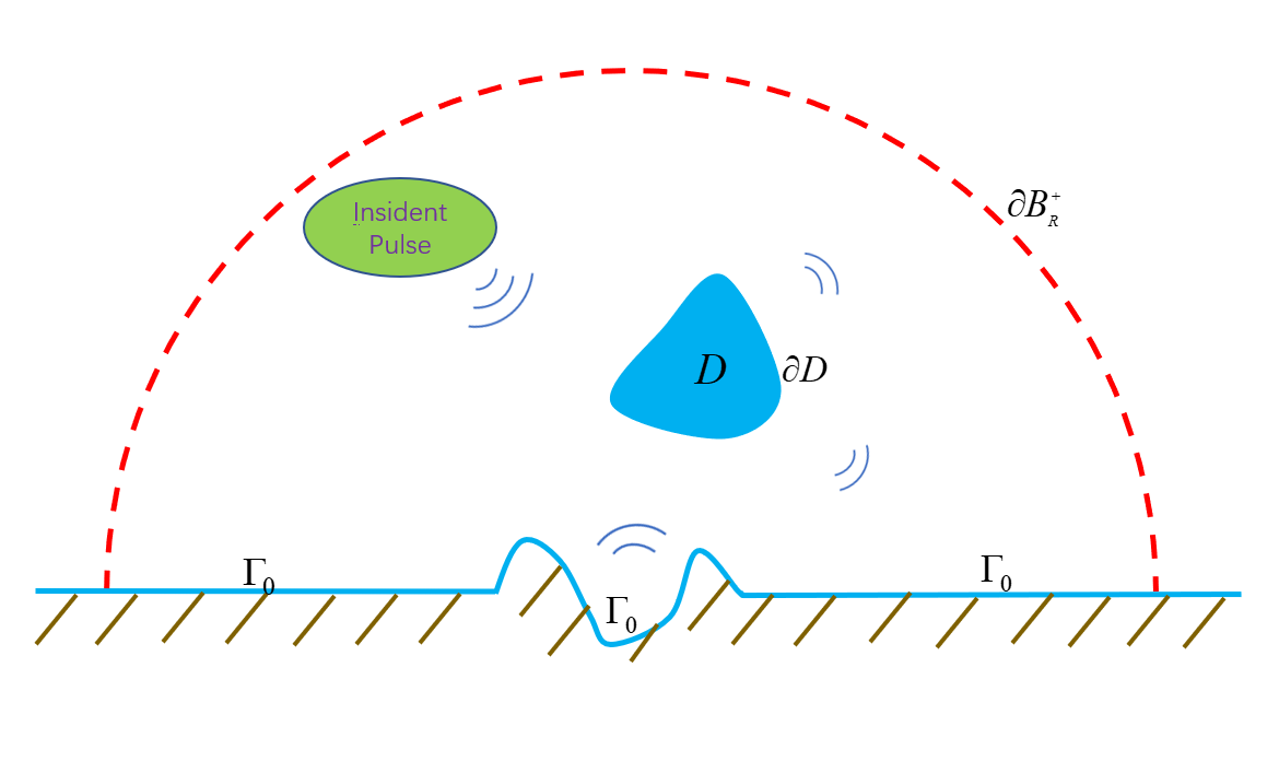
In this work, a perturbation of the half plane $\{x:x_{2}>0\}$ can be caused by either a bounded obstacle imbedded in the background medium or a compact change of the unbounded curve $x_{2}=0$ ; see the geometry shown in Figure 1. Firstly, we adopt the approach of [19] to prove well-posedness of the scattering problem in proper time-dependent Sobolev spaces by using a well-defined TBC (Dirichlet-to-Neumann operator). We complement the earlier work [19] by describing mapping properties of the DtN operator and by connecting the TBCs defined over a finite and an infinite time period, which seem not well-addressed in the literature. Motivated by [19], a circular PML layer with special medium properties will then be defined to truncate the original problem. A first order symmetric hyperbolic system is derived for the truncated PML problem, which is similar to those considered in [19, 20, 6]. The well-posedness and stability of the truncated PML problem are justified by Laplace transform, variational method together with the energy method of [10]. The convergence of the PML scheme is based on the stability estimate of an initial-boundary value problem in the PML layer and the exponential decay of the PML extension problem to be proved using modified Bessel functions. Such a technique is also inspired [19].

This paper is organized as follows. In the subsequent Section 2, we first introduce the mathematical model and rigorous define the transparent boundary condition (TBC) to reformulate the scattering problem to an initial-boundary value problem in a truncated bounded domain. Well-posedness and stability will then be shown in Section 2.2. In Section 3, we derive a PML formulation in the half plane by complex coordinates stretching inspired by [16, 19, 20, 34] and study the well-posedness and stability for the PML problem. We analyze the exponential convergence of the PML method in the half space in Section 4. In the final Section 5, two numerical examples are reported to show the performance of the PML method.

2 Mathematical formulations

Let $\Gamma_{0}$ be a local perturbation of the straight line $\{(x_{1},0):x_{1}\in{\mathbb{R}}\}$ such that $\Gamma_{0}$ coincides with $x_{2}=0$ in $|x_{1}|>R$ for some $R>0$ and that $\Gamma_{0}$ is a non-selfintersecting $C^{2}$ -smooth curve. Denote by $\Omega\subset{\mathbb{R}}^{2}$ the unbounded domain above $\Gamma_{0}$ , which is supposed to be filled by a homogeneous and isotropic medium with the unit mass density. Let $D\subset B_{R}^{+}:=\{x\in\Omega:|x|<R\}$ be a bounded domain with the Lipschitz boundary $\partial D$ such that the exterior of $D$ is connected; see Figure 1. Physically, the domain $D$ represents a sound soft obstacle embedded in $\Omega$ . Write ${\mathbb{R}}^{2}_{+}=\{x\in{\mathbb{R}}^{2}:x_{2}>0\}$ , $\Gamma_{R}^{+}:=\{x\in\Omega:|x|=R\}$ . It is obvious that $B_{R}^{+}$ is a Lipschitz domain.

The time-dependent acoustic scattering problem with the Dirichlet boundary condition enforcing on the obstacle $\partial D$ and the locally perturbed rough surface $\Gamma_{0}$ can be governed by the initial-boundary value problem of the wave equation

\displaystyle\left\{\begin{array}[]{lll}\partial_{t}^{2}u(x,t)-\Delta u(x,t)=\partial_{t}f(x,t)&&\mbox{in}\quad(\Omega\backslash\overline{D})\times(0,T),\\ u(x,t)=0&&\mbox{on}\quad(\partial D\cup\Gamma_{0})\times(0,T),\\ u(x,0)=\partial_{t}u(x,0)=0&&\mbox{in}\quad(\Omega\backslash\overline{D}).\end{array}\right.

(2.4)

Here, $T>0$ is an arbitrarily fixed positive number, the function $f$ represents an acoustic source term compactly supported in $B_{R}^{+}\backslash\overline{D}$ and $u$ denotes the total field. In the exterior of $B_{R}^{+}$ , the total field $u=u^{in}+u^{re}+u^{sc}$ can be divided into the sum of the incident field $u^{in}$ , the reflected field $u^{re}$ corresponding to the unperturbed scattering problem in the homogeneous half space $x_{2}>0$ and the scattered field $u^{sc}$ caused by $D$ and the perturbation of the straight line $x_{2}=0$ . The first two components of $u$ will be explained as follows.

Refer to caption — Figure 1: Geometry of acoustic wave scattering problem caused by a bounded obstacle $D$ and a locally perturbed curve $\Gamma_{0}$ .

The incident field $u^{in}$ is generated by the inhomogeneous wave equation in ${\mathbb{R}}^{2}$ :

\displaystyle\left\{\begin{array}[]{lll}\partial_{t}^{2}u(x,t)-\Delta u(x,t)=\partial_{t}f(x,t)&&\mbox{in}\quad{\mathbb{R}}^{2},\;t>0,\\ u(x,0)=\partial_{t}u(x,0)=0&&\mbox{in}\quad{\mathbb{R}}^{2}.\end{array}\right.

Obviously, the incident field $u^{in}$ takes the explicit form

\displaystyle u^{in}(x,t)=\int_{{\mathbb{R}}^{2}}G(x,t;\,y)*\partial_{t}f(y,t)\,dy\quad\mbox{in}\quad{\mathbb{R}}^{2}\times{\mathbb{R}}^{+},

where $*$ denotes convolution between $G$ and $\partial_{t}f$ with respect to the time $t$ , and

\displaystyle G(x,t;\,y):=\frac{H(t-|x-y|)}{2\pi\sqrt{t^{2}-|x-y|^{2}}},

is the Green’s function of the wave operator $\partial_{t}^{2}-\Delta$ in the free space ${\mathbb{R}}^{2}\times{\mathbb{R}}$ . Note that $H$ is the Heaviside function defined by

\displaystyle H(t):=\left\{\begin{array}[]{lll}0,&&t\leq 0,\\ 1,&&t>0.\end{array}\right.

The reflected field $u^{re}$ caused by the incident field $u^{in}$ and the Dirichlet curve $x_{2}=0$ is governed by

\displaystyle\left\{\begin{array}[]{lll}\partial_{t}^{2}u^{re}(x,t)-\Delta u^{re}(x,t)=0&&\mbox{in}\quad{\mathbb{R}}^{2}_{+},\;t>0,\\ u^{re}(x,0)=\partial_{t}u^{re}(x,0)=0&&\mbox{in}\quad{\mathbb{R}}^{2}_{+},\\ u^{re}(x,t)=-u^{in}(x,t)&&\mbox{on}\quad x_{2}=0,t>0.\end{array}\right.

Denote by $y^{*}=(y_{1},-y_{2})$ the reflection of $y=(y_{1},y_{2})$ by the straight line $x_{2}=0$ . Through simple calculations, we obtain the expression of the reflected field $u^{re}$ by

	$\displaystyle u^{re}(x,t)$	$\displaystyle=$	$\displaystyle-\int_{{\mathbb{R}}^{2}}G(x,t;\,y^{})\partial_{t}f(y,t)\,dy$
		$\displaystyle=$	$\displaystyle-\int_{0}^{t}\int_{B_{R}^{+}\backslash\overline{D}}G(x-y^{*},t-\tau)\partial\tau f(y,\tau)\,dyd\tau.$

Evidently, the sum $u^{in}+u^{re}$ denotes the total field to the unperturbed scattering problem that corresponds to $u^{in}$ and the Dirichlet curve $x_{2}=0$ . The function $u^{sc}$ consists of the scattered wave from the bounded domain $D$ and the local perturbation $\{x\in\Gamma_{0}:x_{2}\neq 0,x_{1}\in{\mathbb{R}}\}$ .

Throughout this paper, we suppose that for any bounded domain $\Omega_{0}$ , $f\in H^{2}(0,T;L^{2}(\Omega_{0}))$ and that $f|_{t=0}=0$ , $f=\tilde{f}|_{(0,T)}$ where

\displaystyle\tilde{f}\in H^{2}(0,\infty;L^{2}(\Omega_{0})),\quad\|\tilde{f}\|_{H^{2}(0,\infty;L^{2}(\Omega_{0}))}\leq\|f\|_{H^{2}(0,T;L^{2}(\Omega_{0}))}.

This implies that the source term $\partial_{t}f$ on the right hand side of (2.4) belongs to $H^{1}(0,T;\Omega\backslash\overline{D})$ . Hence, applying the approach of J. L. Lions (see [32, Theorem 8.1, Chapter 3] and [32, Theorem 8.2, Chapter 3]) there exists a unique solution $u\in C(0,T;H^{1}_{0}(\Omega\backslash\overline{D}))\cap C^{1}(0,T;L^{2}(\Omega\backslash\overline{D}))$ to (2.4).

2.1 A transparent boundary condition (TBC) on a semi-circle

The aim of this section is to rigorously address the Dirichlet-to-Neumann map for the wave equation (2.4) in a locally perturbed half-plane. We shall follow the spirit of [19] for a bounded sound-hard obstacle but complement the definition of DtN there by describing mapping properties in time-dependent Sobolev spaces and connecting the DtN operators defined over a finite and an infinite time period. More precisely, we shall define the time-domain boundary operator $\mathscr{T}$ by

\displaystyle\mathscr{T}u=\partial_{r}u\quad\mbox{on}\quad\Gamma_{R}^{+}\times(0,T),

(2.8)

which is called the TBC. Thus, the time-domain scattering problem (2.4) in the unbounded domain over the local rough surface can be reduced into an equivalent initial-boundary value problem in the bounded domain $\Omega_{R}^{+}:=B_{R}^{+}\backslash\overline{D}$ :

\displaystyle\left\{\begin{array}[]{lll}\partial_{t}^{2}u-\Delta u=\partial_{t}f&&\mbox{in}\quad\Omega_{R}^{+}\times(0,T),\\ u=0&&\mbox{on}\quad(\partial D\cup\Gamma_{0})\times(0,T),\\ \partial_{r}u=\mathscr{T}u&&\mbox{on}\quad\Gamma_{R}^{+}\times(0,T),\\ u|_{t=0}=\partial_{t}u|_{t=0}=0&&\mbox{in}\quad\Omega_{R}^{+}.\end{array}\right.

(2.13)

In what follows we derive a representation of the boundary operator $\mathscr{T}$ . Let $H^{1/2}_{0}(\Gamma_{R}^{+})$ , $H^{1/2}(\Gamma_{R}^{+})$ , $H^{-1/2}(\Gamma_{R}^{+})$ , $H^{-1/2}_{0}(\Gamma_{R}^{+})$ be Sobolev spaces defined on the open arc $\Gamma_{R}^{+}$ . Then $H^{1/2}_{0}(\Gamma_{R}^{+})$ and $H^{-1/2}(\Gamma_{R}^{+})$ , $H^{1/2}(\Gamma_{R}^{+})$ and $H^{-1/2}_{0}(\Gamma_{R}^{+})$ are anti-linear dual spaces[33]. For $u\in H^{1}_{0}(B_{R}^{+})$ , we have $u|_{\Gamma_{R}^{+}}\in H^{1/2}_{0}(\Gamma_{R}^{+})$ .

Consider an initial-boundary value problem over a finite time period

\displaystyle\left\{\begin{array}[]{lll}\partial_{t}^{2}u(x,t)-\Delta u(x,t)=0&&\mbox{in}\quad(\Omega\backslash\overline{B_{R}^{+}})\times(0,T),\\ u(x,t)=g(x,t)&&\mbox{on}\quad\Gamma_{R}^{+}\times(0,T),\\ u(x,t)=0&&\mbox{on}\quad(\Gamma_{0}\cap|x|>R)\times(0,T),\\ u(x,0)=\partial_{t}u(x,0)=0&&\mbox{in}\quad(\Omega\backslash\overline{B_{R}^{+}})\end{array}\right.

(2.18)

where $g\in C(0,T;H^{1/2}_{0}(\Gamma_{R}^{+}))\,\cap C^{1}(0,T;H^{-1/2}(\Gamma_{R}^{+}))$ satisfying $g(x,0)=\partial_{t}g(x,0)=0$ . By [15, Chapter 7], there exists a unique solution $u$ to the above equations satisfying

\displaystyle u\in C(0,T;H^{1}_{\diamond}(\Omega\backslash\overline{B_{R}^{+}}))\cap C^{1}(0,T;L^{2}(\Omega\backslash\overline{B_{R}^{+}})),

where $H^{1}_{\diamond}(\Omega\backslash\overline{B_{R}^{+}})=\{u\in H^{1}(\Omega\backslash B_{R}^{+}):u=0\;\mbox{on}\;\{\Gamma_{0}\cap|x|>R\}\}$ .

Definition 2.1.

The DtN operator $\mathscr{T}:C(0,T;H^{1/2}_{0}(\Gamma_{R}^{+}))\rightarrow C(0,T;H^{-1/2}(\Gamma_{R}^{+}))$ over a finite time period $(0,T)$ is defined as

\displaystyle\mathscr{T}g=\partial_{r}u\quad\mbox{on}\quad\Gamma_{R}^{+}\times(0,T),

where $u\in C(0,T;H^{1}_{\diamond}(\Omega\backslash\overline{B_{R}^{+}}))\cap C^{1}(0,T;L^{2}(\Omega\backslash\overline{B_{R}^{+}}))$ is the unique solution to (2.18).

Consider another initial-boundary value problem but over an infinite time

\displaystyle\left\{\begin{array}[]{lll}\partial_{t}^{2}w(x,t)-\Delta w(x,t)=0&&\mbox{in}\quad(\Omega\backslash\overline{B_{R}^{+}})\times(0,\infty),\\ w(x,t)=\tilde{g}(x,t)&&\mbox{on}\quad\Gamma_{R}^{+}\times(0,\infty),\\ w(x,t)=0&&\mbox{on}\quad(\Gamma_{0}\cap|x|>R)\times(0,\infty),\\ w(x,0)=\partial_{t}w(x,0)=0&&\mbox{in}\quad(\Omega\backslash\overline{B_{R}^{+}}),\end{array}\right.

(2.23)

with the initial-boundary value

\displaystyle\tilde{g}\in L^{2}(0,\infty;H^{1/2}_{0}(\Gamma_{R}^{+}))\,\cap H^{1}(0,\infty;H^{-1/2}(\Gamma_{R}^{+})),\quad\tilde{g}(x,0)=\partial_{t}\tilde{g}(x,0)=0.

(2.24)

Definition 2.2.

The DtN operator $\tilde{\mathscr{T}}:L^{2}(0,\infty;H^{1/2}_{0}(\Gamma_{R}^{+}))\rightarrow L^{2}(0,\infty;H^{-1/2}(\Gamma_{R}^{+}))$ over the infinite time period $(0,\infty)$ is defined as

\displaystyle\tilde{\mathscr{T}}\tilde{g}=\partial_{r}w\quad\mbox{on}\quad\Gamma_{R}^{+}\times(0,\infty),

where $w\in L^{2}(0,\infty;H^{1}_{\diamond}(\Omega\backslash\overline{B_{R}^{+}}))\cap H^{1}(0,\infty;L^{2}(\Omega\backslash\overline{B_{R}^{+}}))$ is the unique solution of (2.23).

Lemma 2.1.

Let $\tilde{g}$ be the boundary value of the problem (2.18) and denote by $\tilde{g}$ its zero extension to $t>T$ . Then

\displaystyle\tilde{\mathscr{T}}\tilde{g}=\mathscr{T}g\quad\mbox{in}\quad L^{2}(0,T;H^{-1/2}(\Gamma_{R}^{+})).

Proof.

It is obvious that the extension $\tilde{g}$ fulfills the regularity and initial values specified in (2.24). Define $v:=u-w$ , where $u$ and $w$ are the unique solutions to (2.18) and (2.23), respectively. It then follows that

\displaystyle\left\{\begin{array}[]{lll}\partial_{t}^{2}v(x,t)-\Delta v(x,t)=0&&\mbox{in}\quad(\Omega\backslash\overline{B_{R}^{+}})\times(0,T),\\ v(x,t)=0&&\mbox{on}\quad\Gamma_{R}^{+}\times(0,T),\\ v(x,t)=0&&\mbox{on}\quad(\Gamma_{0}\cap|x|>R)\times(0,T),\\ v(x,0)=\partial_{t}v(x,0)=0&&\mbox{in}\quad(\Omega\backslash\overline{B_{R}^{+}}).\end{array}\right.

(2.29)

By uniqueness to the above system (see e.g., [32, 15]), we get $v\equiv 0$ in $(\Omega\backslash\overline{B_{R}^{+}})\times(0,T)$ , implying that $\partial_{r}v=0$ on $\Gamma_{R}^{+}\times(0,T)$ . Hence, we obtain that $\tilde{\mathscr{T}}\tilde{g}=\mathscr{T}g$ on $\Gamma_{R}^{+}\times(0,T)$ . ∎

From the proof of Lemma 2.1 we conclude that the definition of $\mathscr{T}g$ is independent of the values of $g$ in $t>T$ . Below we want to derive an expression of $\tilde{\mathscr{T}}$ by Laplace transform. For any $s\in{\mathbb{C}}$ with $\textnormal{Re}(s)>0$ , applying Laplace transform to (2.23) with respect to $t$ , we see that $w_{L}=\mathscr{L}(w)$ satisfies the Helmoholtz equation

\displaystyle-\Delta w_{L}+s^{2}w_{L}=0\quad\mbox{in}\quad\Omega\backslash\overline{B_{R}^{+}},

(2.30)

together with the radiation condition

\displaystyle\sqrt{r}(\frac{\partial w_{L}}{\partial r}+sw_{L})\rightarrow 0\quad\mbox{as}\quad r=|x|\rightarrow\infty.

(2.31)

Let $\mathscr{G}:H^{1/2}_{0}(\Gamma_{R}^{+})\rightarrow H^{-1/2}(\Gamma_{R}^{+})$ be the DtN operator in s-domain defined by

\displaystyle\mathscr{G}\tilde{g}_{L}=\partial_{r}w_{L}\quad\textnormal{on}\quad\Gamma_{R}^{+}.

where $w_{L}$ is the unique solution to (2.30)-(2.31) satisfying the boundary value $w_{L}=g_{L}$ on $\Gamma_{R}^{+}$ and $w_{L}=0$ on $\Gamma_{0}\cap\{x:|x|>R\}$ . Then it follows that

\tilde{\mathscr{T}}=\mathscr{L}^{-1}\circ\mathscr{G}\circ\mathscr{L}.

Next, we derive a representation of the DtN operator $\mathscr{G}$ . In the polar coordinates $(r,\theta)$ , $w_{L}$ can be expanded into the series (see e.g., [19, 30, 39])

\displaystyle w_{L}(r,\theta;s)=\sum_{n=1}^{\infty}\frac{K_{n}(sr)}{K_{n}(sR)}w^{n}_{L}(R,s)\sin{n\theta},\quad r>R,\quad\theta\in[0,\pi],

where

w^{n}_{L}(R,s)=\frac{2}{\pi}\int_{0}^{\pi}{w_{L}(R,\theta,s)\sin{n\theta}\,d\theta}=\frac{2}{\pi}\int_{0}^{\pi}{\tilde{g}_{L}(R,\theta,s)\sin{n\theta}\,d\theta}.

Here $K_{n}(z)$ represents the modified Bessel function of order $n$ . A simple calculation gives

\displaystyle\mathscr{G}w_{L}(R,\theta,s)=\frac{\partial w_{L}}{\partial r}|_{\Gamma_{R}^{+}}=s\sum_{n=1}^{\infty}\frac{K_{n}^{\prime}(sR)}{K_{n}(sR)}w^{n}_{L}(R,s)\sin{n\theta}.

(2.32)

The DtN operators $\mathscr{G}$ and $\mathscr{T}$ have the following properties.

Lemma 2.2.

The operator $\mathscr{G}:H^{1/2}_{0}(\Gamma_{R}^{+})\rightarrow H^{-1/2}(\Gamma_{R}^{+})$ is bounded.

Proof.

By the recurrence formula of modified Bessel function

\displaystyle K_{n}^{{}^{\prime}}(z)=-K_{n-1}(z)-\frac{n}{z}K_{n}(z),

we deduce that

\displaystyle\Big{|}\frac{K_{n}^{{}^{\prime}}(sR)}{K_{n}(sR)}\Big{|}=\Big{|}\frac{n}{sR}+\frac{K_{n-1}(sR)}{K_{n}(sR)}\Big{|}\leq\frac{n}{|s|R}+1.

Let $|B_{n}|:=\Big{|}\frac{K_{n}^{{}^{\prime}}(sR)}{K_{n}(sR)}\Big{|}$ . Then, $|B_{n}|\leq C\sqrt{n^{2}+1}$ for some constant $C>0$ . Given $\phi\in H^{-1/2}_{0}(\Gamma_{R}^{+})$ , we expand

\displaystyle\phi(R,\theta)=\sum_{n=1}^{\infty}\phi_{n}(R)\sin{n\theta},\quad\phi_{n}(R)=\frac{2}{\pi}\int_{0}^{\pi}\phi(R,\theta)\sin n\theta\,d\theta.

By the definition of $\mathscr{G}$ , for any $\omega\in H^{1/2}_{0}(\Gamma_{R}^{+})$ it follows that

	$\displaystyle\Big{\|}\langle\mathscr{G}(\omega),\,\phi\rangle_{\Gamma_{R}^{+}}\Big{\|}$	$\displaystyle=\Big{\|}\int_{\Gamma_{R}^{+}}s\sum_{n=1}^{\infty}\frac{K_{n}^{{}^{\prime}}(sR)}{K_{n}(sR)}\omega_{n}(R)\sin n\theta\sum_{n=1}^{\infty}\overline{\phi}_{n}(R)\sin n\theta\,d\gamma\Big{\|}$
		$\displaystyle=\Big{\|}sR\sum_{n=1}^{\infty}\frac{K_{n}^{{}^{\prime}}(sR)}{K_{n}(sR)}\omega_{n}(R)\overline{\phi}_{n}(R)\int_{0}^{\pi}\sin^{2}n\theta\,d\theta$
		$\displaystyle=\Big{\|}\frac{\pi}{2}sR\sum_{n=1}^{\infty}\frac{K_{n}^{{}^{\prime}}(sR)}{K_{n}(sR)}\omega_{n}(R)\overline{\phi}_{n}(R)\Big{\|}$
		$\displaystyle\leq\frac{\pi}{2}\|s\|R\Big{(}\sum_{n=1}^{\infty}\Big{\|}\frac{K_{n}^{{}^{\prime}}(sR)}{K_{n}(sR)}\Big{\|}\|\omega_{n}(R)\|^{2}\Big{)}^{1/2}\Big{(}\sum_{n=1}^{\infty}\Big{\|}\frac{K_{n}^{{}^{\prime}}(sR)}{K_{n}(sR)}\Big{\|}\|\phi_{n}(R)\|^{2}\Big{)}^{1/2}$
		$\displaystyle\leq C\Big{(}\sum_{n=1}^{\infty}\sqrt{1+n^{2}}\|\omega_{n}(R)\|^{2}\Big{)}^{1/2}\Big{(}\sum_{n=1}^{\infty}\sqrt{1+n^{2}}\|\phi_{n}(R)\|^{2}\Big{)}^{1/2}$
		$\displaystyle\leq C\\|\omega\\|_{H^{1/2}_{0}(\Gamma_{R}^{+})}\,\\|\phi\\|_{H^{1/2}_{0}(\Gamma_{R}^{+})}.$

Then, we have

\displaystyle\|\mathscr{G}\omega\|_{H^{-1/2}(\Gamma_{R}^{+})}=\sup_{\phi\in H^{1/2}_{0}(\Gamma_{R}^{+})}\frac{\Big{|}\langle\mathscr{G}(\omega),\,\phi\rangle_{\Gamma_{R}^{+}}\Big{|}}{\|\phi\|_{H^{1/2}_{0}(\Gamma_{R}^{+})}}\leq C\|\omega\|_{H^{1/2}_{0}(\Gamma_{R}^{+})}.

∎

Lemma 2.3.

It holds that, for any $\omega\in H^{1/2}_{0}(\Gamma_{R}^{+})$ ,

\displaystyle-\textnormal{Re}\,\langle s^{-1}\,\mathscr{G}\omega,\,\omega\rangle_{\Gamma_{R}^{+}}\geq 0.

Proof.

Given $\omega\in H^{1/2}_{0}(\Gamma_{R}^{+})$ , we have

\displaystyle\omega(R,\theta)=\sum_{n=1}^{\infty}\omega_{n}(R)\sin{n\theta},\quad\omega_{n}(R)=\frac{2}{\pi}\int_{0}^{\pi}\omega(R,\theta)\sin n\theta\,d\theta.

It follows from the expression of $\mathscr{G}u_{L}$ (2.32) and Lemma C.1, we obtain

	$\displaystyle-\textnormal{Re}\,\langle s^{-1}\,\mathscr{G}\omega,\omega\rangle_{\Gamma_{R}^{+}}=$	$\displaystyle-\textnormal{Re}\int_{\Gamma_{R}^{+}}\sum_{n=1}^{\infty}\frac{K_{n}^{{}^{\prime}}(sR)}{K_{n}(sR)}\omega_{n}(R)\sin n\theta\sum_{n=1}^{\infty}\overline{\omega}_{n}(R)\sin n\theta\,d\gamma$
	$\displaystyle=$	$\displaystyle-R\sum_{n=1}^{\infty}\textnormal{Re}\Big{(}\frac{K_{n}^{{}^{\prime}}(sR)}{K_{n}(sR)}\Big{)}\|\omega_{n}(R)\|^{2}\int_{0}^{\pi}\sin^{2}n\theta\,d\theta$
	$\displaystyle=$	$\displaystyle-\frac{\pi}{2}R\sum_{n=1}^{\infty}\textnormal{Re}\Big{(}\frac{K_{n}^{{}^{\prime}}(sR)}{K_{n}(sR)}\Big{)}\|\omega_{n}(R)\|^{2}\geq 0.$

∎

Below we write the Laplace transform variable as $s=s_{1}+is_{2}$ with $s_{1}>0$ , $s_{2}\in{\mathbb{R}}$ .

Lemma 2.4.

Let $\omega\in C(0,T;H^{1/2}_{0}({\Gamma_{R}^{+}})\cap C^{1}(0,T;H^{-1/2}({\Gamma_{R}^{+}})$ with the initial values $\omega(\cdot,\,0)=\partial_{t}\omega(\cdot,\,0)=0$ . Then it holds that

\displaystyle\textnormal{Re}\,\int_{0}^{T}e^{-2s_{1}t}\langle\mathscr{T}\omega,\,\partial_{t}\omega\rangle_{\Gamma_{R}^{+}}\,dt\leq 0.

Proof.

Let $\tilde{\omega}(r,t)$ be the zero extension of $\omega(r,t)$ with respect to $t$ in ${\mathbb{R}}$ . Applying the Parseval identity (A.4) and Lemmas 2.1 and 2.3, we obtain

	$\displaystyle\textnormal{Re}\,\int_{0}^{T}e^{-2s_{1}t}\langle\mathscr{T}\omega,\,\partial_{t}\omega\rangle_{\Gamma_{R}^{+}}\,dt$	$\displaystyle=\textnormal{Re}\,\int_{0}^{T}e^{-2s_{1}t}\int_{\Gamma_{R}^{+}}\mathscr{T}\omega\partial_{t}\overline{\omega}\,d\gamma\,dt$
		$\displaystyle=\textnormal{Re}\,\int_{\Gamma_{R}^{+}}\int_{0}^{\infty}e^{-2s_{1}t}\tilde{\mathscr{T}}\tilde{\omega}\partial_{t}\overline{\tilde{\omega}}\,dt\,d\gamma$
		$\displaystyle=\frac{1}{2\pi}\int_{-\infty}^{\infty}\textnormal{Re}\langle\mathscr{G}\tilde{\omega}_{L},\,s\tilde{\omega}_{L}\rangle_{\Gamma_{R}^{+}}\,ds_{2}$
		$\displaystyle=\frac{1}{2\pi}\int_{-\infty}^{\infty}\|s\|^{2}\textnormal{Re}\langle s^{-1}\mathscr{G}\tilde{\omega}_{L},\,\tilde{\omega}_{L}\rangle_{\Gamma_{R}^{+}}\,ds_{2}$
		$\displaystyle\leq 0.$

∎

2.2 Well-posedness in the time-domain

In the subsection, we prove well-posedness of the truncated initial-boundary value problem (2.13) in the bounded domain $\Omega_{R}^{+}$ by using the variational method in the Laplace domain. Taking Laplace transform of (2.13) and using $f(\cdot,0)=0$ we obtain

\displaystyle\left\{\begin{array}[]{lll}\Delta u_{L}-s^{2}u_{L}=sf_{L}&&\mbox{in}\quad\Omega_{R}^{+}\backslash\overline{D},\\ u_{L}=0&&\mbox{on}\quad\partial D\cup\Gamma_{0},\\ \partial_{r}u_{L}=\mathscr{G}u_{L}&&\mbox{on}\quad\Gamma_{R}^{+}.\end{array}\right.

(2.36)

We formulate the variational formulation of problem (2.36) and show its well-posedness in the space $X_{R}:=\{u\in H^{1}(\Omega_{R}^{+}):u=0\;\mbox{on}\;\partial D\cup\Gamma_{0}\}$ . Multiplying the Helmholtz equation in (2.36) by the complex conjugate of a test function $v\in X_{R}$ , applying the Green’s formula with the boundary conditions on $\Gamma_{R}^{+}\cup\Gamma_{0}\cup\partial D$ , we arrive at

\displaystyle a(u_{L},\,v)=\int_{\Omega_{R}^{+}}f_{L}\,\overline{v}\,dx\quad\mbox{for all}\quad v\in X_{R},

(2.37)

where the sesquilinear form $a(\cdot,\cdot)$ is defined as

\displaystyle a(u_{L},\,v)=\int_{\Omega_{R}^{+}}\left(\frac{1}{s}\nabla u_{L}\cdot\nabla\overline{v}+su_{L}\overline{v}\right)\,dx-\langle s^{-1}\mathscr{G}u_{L},\,v\rangle_{\Gamma_{R}^{+}}.

Lemma 2.5.

The variational problem (2.37) has a unique solution $u_{L}\in X_{R}$ with the following stability estimate

\displaystyle\|\nabla u_{L}\|_{L^{2}(\Omega_{R}^{+})}+\|su_{L}\|_{L^{2}(\Omega_{R}^{+})}\leq C\frac{(1+|s|)|s|}{s_{1}}\|f_{L}\|_{L^{2}(\Omega_{R}^{+})},

(2.38)

where $C$ is a constant independent of $s$ .

Proof.

(i) We first prove that $a(\cdot,\,\cdot)$ is continuous and strictly coercive. Using the Cauchy-Schwarz inequality, the boundedness of $\mathscr{G}$ in Lemma 2.2 and the trace theorem, we obtain

$\displaystyle\|a(u_{L},\,v)\|$	$\displaystyle\leq$	$\displaystyle\|s\|^{-1}\\|\nabla u_{L}\\|_{L^{2}(\Omega_{R}^{+})}\\|\nabla v\\|_{L^{2}(\Omega_{R}^{+})}+\|s\|\\|u_{L}\\|_{L^{2}(\Omega_{R}^{+})}\\|v\\|_{L^{2}(\Omega_{R}^{+})}$
		$\displaystyle+\|s\|^{-1}\\|\mathscr{G}u_{L}\\|_{H^{-1/2}(\Gamma_{R}^{+})}\\|v\\|_{H^{1/2}(\Gamma_{R}^{+})}$
	$\displaystyle\leq$	$\displaystyle C\\|u_{L}\\|_{H^{1}(\Omega_{R}^{+})}\\|v\\|_{H^{1}(\Omega_{R}^{+})}+C\\|u_{L}\\|_{H^{1}(\Omega_{R}^{+})}\\|v\\|_{H^{1}(\Omega_{R}^{+})}$
		$\displaystyle C\\|u_{L}\\|_{H^{1/2}(\Gamma_{R}^{+})}\\|v\\|_{H^{1/2}(\Gamma_{R}^{+})}$
	$\displaystyle\leq$	$\displaystyle C\\|u_{L}\\|_{H^{1}(\Omega_{R}^{+})}\\|v\\|_{H^{1}(\Omega_{R}^{+})}.$

Setting $v=u_{L}$ , it follows from the expression of the sesquilinear form $a(\cdot,\cdot)$ that

\displaystyle a(u_{L},\,u_{L})=\int_{\Omega_{R}^{+}}\frac{1}{s}|\nabla u_{L}|^{2}+s|u_{L}|^{2}\,dx-\langle s^{-1}\mathscr{G}u_{L},\,u_{L}\rangle_{\Gamma_{R}^{+}}.

Taking the real part of the above equation and using Lemma 2.3 we have

$\displaystyle\textnormal{Re}(a(u_{L},\,u_{L}))$	$\displaystyle=$	$\displaystyle\int_{\Omega_{R}^{+}}\frac{s_{1}}{\|s\|^{2}}\|\nabla u_{L}\|^{2}+s_{1}\|u_{L}\|^{2}\,dx-\textnormal{Re}\langle s^{-1}\mathscr{G}u_{L},\,u_{L}\rangle_{\Gamma_{R}^{+}}$	(2.39)
	$\displaystyle\geq$	$\displaystyle\int_{\Omega_{R}^{+}}\frac{s_{1}}{\|s\|^{2}}\|\nabla u_{L}\|^{2}+s_{1}\|u_{L}\|^{2}\,dx$
	$\displaystyle\geq$	$\displaystyle\frac{s_{1}}{\|s\|^{2}}\left(\\|\nabla u_{L}\\|_{L^{2}(\Omega_{R}^{+})}^{2}+\\|su_{L}\\|_{L^{2}(\Omega_{R}^{+})}^{2}\right).$

Hence, by the Lax-Milgram Lemma, the variational problem (2.37) has a unique solution $u_{L}\in X_{R}$ .

(ii) Combining (2.37) with the Cauchy-Schwarz inequality, it follows that

$\displaystyle\|a(u_{L},\,u_{L})\|$	$\displaystyle\leq$	$\displaystyle\frac{1}{\|s\|}\\|f_{L}\\|_{L^{2}(\Omega_{R}^{+})}\\|su_{L}\\|_{L^{2}(\Omega_{R}^{+})}$	(2.40)
	$\displaystyle\leq$	$\displaystyle\frac{1}{\|s\|}\\|f_{L}\\|_{L^{2}(\Omega_{R}^{+})}\\|su_{L}\\|_{H^{1}(\Omega_{R}^{+})}$
	$\displaystyle\leq$	$\displaystyle\frac{1}{\|s\|}\\|f_{L}\\|_{L^{2}(\Omega_{R}^{+})}\left(\|s\|^{2}\\|\nabla u_{L}\\|_{L^{2}(\Omega_{R}^{+})}^{2}+\\|su_{L}\\|_{L^{2}(\Omega_{R}^{+})}^{2}\right)^{1/2}$
	$\displaystyle\leq$	$\displaystyle C\frac{1+\|s\|}{\|s\|}\\|f_{L}\\|_{L^{2}(\Omega_{R}^{+})}\left(\\|\nabla u_{L}\\|_{L^{2}(\Omega_{R}^{+})}^{2}+\\|su_{L}\\|_{L^{2}(\Omega_{R}^{+})}^{2}\right)^{1/2}.$

Combining (2.39) and (2.40) yields

			$\displaystyle\frac{s_{1}}{\|s\|^{2}}\left(\\|\nabla u_{L}\\|_{L^{2}(\Omega_{R}^{+})}^{2}+\\|su_{L}\\|_{L^{2}(\Omega_{R}^{+})}^{2}\right)$
		$\displaystyle\leq$	$\displaystyle\textnormal{Re}(a(u_{L},\,u_{L}))$
		$\displaystyle\leq$	$\displaystyle\|a(u_{L},\,u_{L})\|$
		$\displaystyle\leq$	$\displaystyle C\frac{1+\|s\|}{\|s\|}\\|f_{L}\\|_{L^{2}(\Omega_{R}^{+})}\left(\\|\nabla u_{L}\\|_{L^{2}(\Omega_{R}^{+})}^{2}+\\|su_{L}\\|_{L^{2}(\Omega_{R}^{+})}^{2}\right)^{1/2}.$

Then, using the Cauchy-Schwarz inequality, we have

	$\displaystyle\\|\nabla u_{L}\\|_{L^{2}(\Omega_{R}^{+})}+\\|su_{L}\\|_{L^{2}(\Omega_{R}^{+})}$	$\displaystyle\leq$	$\displaystyle\left(\\|\nabla u_{L}\\|_{L^{2}(\Omega_{R}^{+})}^{2}+\\|su_{L}\\|_{L^{2}(\Omega_{R}^{+})}^{2}\right)^{1/2}$
		$\displaystyle\leq$	$\displaystyle C\frac{(1+\|s\|)\|s\|}{s_{1}}\\|f_{L}\\|_{L^{2}(\Omega_{R}^{+})},$

which completes the proof of the stability estimate. ∎

Theorem 2.1.

The initial boundary value problem (2.13) has a unique solution

\displaystyle u(x,t)\in L^{2}(0,T;X_{R})\cap H^{1}(0,T;L^{2}(\Omega_{R}^{+})),

which satisfies the stability estimate

\displaystyle\max_{0\leq t\leq T}\Big{(}\|\partial_{t}u\|_{L^{2}(\Omega_{R}^{+})}+\|\nabla u\|_{L^{2}(\Omega_{R}^{+})}\Big{)}\leq C\|\partial_{t}f\|_{L^{1}(0,T;L^{2}(\Omega_{R}^{+}))}.

Proof.

We first prove existence and uniqueness of solutions to (2.13). Simple calculations show that

			$\displaystyle\int_{0}^{T}\\|\partial_{t}u\\|_{L^{2}(\Omega_{R}^{+})}^{2}+\\|\nabla u\\|_{L^{2}(\Omega_{R}^{+})}^{2}\,dt$
	$\displaystyle\leq$		$\displaystyle C\int_{0}^{\infty}e^{-2s_{1}t}\Big{(}\\|\partial_{t}u\\|_{L^{2}(\Omega_{R}^{+})}^{2}+\\|\nabla u\\|_{L^{2}(\Omega_{R}^{+})}^{2}\Big{)}\,dt.$

Hence it suffices to estimate the integral

\displaystyle\int_{0}^{\infty}e^{-2s_{1}t}\Big{(}\|\partial_{t}u\|_{L^{2}(\Omega_{R}^{+})}^{2}+\|\nabla u\|_{L^{2}(\Omega_{R}^{+})}^{2}\Big{)}\,dt.

Based on the stability estimate of $u_{L}$ in Lemma 2.5, we derive from [35, Lemma 44.1] that $u_{L}$ is a holomorphic function of $s$ on the half plane $s_{1}>\zeta_{0}>0$ , where $\zeta_{0}$ is any positive constant. Thus, by Lemma A.2, the inverse Laplace transform of $u_{L}$ exists and is supported in $[0,\infty)$ .

Set $u=\mathscr{L}^{-1}(u_{L})$ . Applying the Parseval identity (A.4) and the stability estimate (2.38) in Lemma 2.5 and using the Cauchy-Schwarz inequality, we obtain

			$\displaystyle\int_{0}^{\infty}e^{-2s_{1}t}(\\|\partial_{t}u\\|_{L^{2}(\Omega_{R}^{+})}^{2}+\\|\nabla u\\|_{L^{2}(\Omega_{R}^{+})}^{2})\,dt$
	$\displaystyle=$		$\displaystyle\frac{1}{2\pi}\int_{-\infty}^{+\infty}\\|su_{L}\\|_{L^{2}(\Omega_{R}^{+}}^{2}+\\|\nabla u_{L}\\|_{L^{2}(\Omega_{R}^{+})}^{2})\,ds_{2}$
	$\displaystyle\leq$		$\displaystyle C\frac{1}{s_{1}^{2}}\int_{-\infty}^{+\infty}(1+\|s\|)^{2}\|s\|^{2}\\|f_{L}\\|_{L^{2}(\Omega_{R}^{+})}^{2}\,ds_{2}$
	$\displaystyle\leq$		$\displaystyle C\frac{1}{s_{1}^{2}}\int_{-\infty}^{+\infty}\\|s^{2}f_{L}\\|_{L^{2}(\Omega_{R}^{+})}^{2}+\\|sf_{L}\\|_{L^{2}(\Omega_{R}^{+})}^{2}\,ds_{2}$
	$\displaystyle\leq$		$\displaystyle C\frac{1}{s_{1}^{2}}\int_{0}^{\infty}e^{-2s_{1}t}\left(\\|\partial_{t}^{2}f\\|_{L^{2}(\Omega_{R}^{+})}^{2}+\\|\partial_{t}f\\|_{L^{2}(\Omega_{R}^{+})}^{2}\right)\,dt.$

This together with the Poincaré inequality proves

\displaystyle u\in L^{2}(0,T;X_{R})\cap H^{1}(0,T;L^{2}(\Omega_{R}^{+})).

To prove the stability estimate, we define the energy function

\displaystyle E(t):=\frac{1}{2}\left(\|\partial_{t}u\|_{L^{2}(\Omega_{R}^{+})}^{2}+\|\nabla u\|_{L^{2}(\Omega_{R}^{+})}^{2}\right),\quad 0<t<T.

It is obvious that

\displaystyle E(t)-E(0)=\int_{0}^{t}E^{\prime}(\tau)\,d\tau.

Recalling the wave equation in (2.13) and applying integration by parts, we obtain

$\displaystyle\int_{0}^{t}e^{-2s_{1}\tau}E^{\prime}(\tau)\,d\tau\quad=$	$\displaystyle\mbox{Re}\int_{0}^{t}e^{-2s_{1}\tau}\int_{\Omega_{R}^{+}}\partial_{\tau\tau}u\partial_{\tau}\overline{u}+\nabla u\cdot\nabla(\partial_{\tau}\overline{u})\,dxd\tau$
$\displaystyle=$	$\displaystyle\mbox{Re}\int_{0}^{t}e^{-2s_{1}\tau}\int_{\Omega_{R}^{+}}(\Delta u+\partial_{\tau}f)\partial_{\tau}\overline{u}+\nabla u\cdot\nabla(\partial_{\tau}\overline{u})\,dxd\tau$
$\displaystyle=$	$\displaystyle\mbox{Re}\int_{0}^{t}e^{-2s_{1}\tau}\langle\mathscr{T}u,\,\partial_{\tau}\overline{u}\rangle_{\Gamma_{R}^{+}}\,d\tau$	(2.41)
	$\displaystyle+\mbox{Re}\int_{0}^{t}e^{-2s_{1}\tau}(\partial_{\tau}f,\,\partial_{\tau}\overline{u})_{L^{2}(\Omega_{R}^{+})}\,d\tau.$	(2.41)

Applying integration by parts on the left hand side of (2.2) and using $E(0)=0$ together with Lemma 2.4, we obtain

			$\displaystyle e^{-2s_{1}t}E(t)+2s_{1}\int_{0}^{t}e^{-2s_{1}\tau}E(\tau)\,d\tau$
	$\displaystyle\leq$		$\displaystyle\mbox{Re}\int_{0}^{t}e^{-2s_{1}\tau}(\partial_{\tau}f,\,\partial_{\tau}\overline{u})_{L^{2}(\Omega_{R}^{+})}\,d\tau$
	$\displaystyle\leq$		$\displaystyle\int_{0}^{T}\\|e^{-s_{1}t}\partial_{t}f\\|_{L^{2}(\Omega_{R}^{+})}\,\\|e^{-s_{1}t}\partial_{t}u\\|_{L^{2}(\Omega_{R}^{+})}dt$
	$\displaystyle\leq$		$\displaystyle\max_{0\leq t\leq T}\\|e^{-s_{1}t}\partial_{t}u\\|_{L^{2}(\Omega_{R}^{+})}\,\\|e^{-s_{1}t}\partial_{t}f\\|_{L^{1}(0,T;L^{2}(\Omega_{R}^{+}))}$
	$\displaystyle\leq$		$\displaystyle\varepsilon\max_{0\leq t\leq T}\\|e^{-s_{1}t}\partial_{t}u\\|_{L^{2}(\Omega_{R}^{+})}^{2}+\frac{1}{4\varepsilon}\,\\|e^{-s_{1}t}\partial_{t}f\\|_{L^{1}(0,T;L^{2}(\Omega_{R}^{+}))}^{2}.$

Letting $s_{1}\rightarrow 0$ , choosing $\varepsilon>0$ small enough and applying Cauchy-Schwartz inequality, we finally get

			$\displaystyle\max_{0\leq t\leq T}\Big{(}\\|\partial_{t}u\\|_{L^{2}(\Omega_{R}^{+})}+\\|\nabla u\\|_{L^{2}(\Omega_{R}^{+})}\Big{)}$
	$\displaystyle\leq$		$\displaystyle C\max_{0\leq t\leq T}\Big{(}\\|\partial_{t}u\\|_{L^{2}(\Omega_{R}^{+})}^{2}+\\|\nabla u\\|_{L^{2}(\Omega_{R}^{+})}^{2}\Big{)}^{1/2}$
	$\displaystyle\leq$		$\displaystyle C\\|\partial_{t}f\\|_{L^{1}(0,T;L^{2}(\Omega_{R}^{+}))}.$

This completes the stability estimate. ∎

3 The time-domain PML problem

Inspired by the PML approach for bounded obstacles [19, 20], we present in this section the time-domain PML formulation in a perturbed half-plane and then show the well-posedness and stability of the PML problem by applying the Laplace transform together with the variational and energy methods.

3.1 Well-posedness of the PML problem

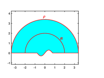
We surround the domain $\Omega_{R}^{+}$ with a PML layer

\Omega_{PML}^{+}:=B_{\rho}^{+}\backslash\overline{B_{R}^{+}}=:\{x\in\Omega:R<|x|<\rho\},

where $B_{\rho}^{+}:=\{x\in\Omega:|x|<\rho\}$ . We denote $\Omega_{\rho}^{+}:=B_{\rho}^{+}\backslash\overline{D}$ the truncated PML domain with the exterior boundary $\Gamma_{\rho}^{+}:=\{x\in\Omega:|x|=\rho\}$ . Let $s_{1}=\textnormal{Re}(s)>0$ for $s\in{\mathbb{C}}$ . Define the medium parameter in the PML layer as

\displaystyle\alpha(r)=\left\{\begin{array}[]{lll}1,&&r\leq R,\\ 1+s^{-1}\sigma(r),&&r>R,\end{array}\right.

where $r=|x|$ , $\sigma=0$ for $r\leq R$ and $\sigma>0$ for $r>R$ .

In what follows, we will derive the PML formulation by a complex transformation of variables. Denote by $\tilde{r}$ the complex radius

\displaystyle\tilde{r}=\int_{0}^{r}\alpha(\tau)\,d\tau=r\beta(r),

where $\beta(r)=r^{-1}\int_{0}^{r}\alpha(\tau)\,d\tau$ . It is obvious that $\beta(r)=1+s^{-1}\hat{\sigma}(r)$ for $r\geq R$ , where $\hat{\sigma}(r)=r^{-1}\int_{0}^{r}\sigma(\tau)\,d\tau$ . To derive the PML equations, we need to transform the exterior problem (2.13) into the s-domain. On $\Gamma_{R}^{+}$ , the Laplace transform of $u$ can be expanded into the series,

\displaystyle u_{L}(R,s)=\sum_{n=1}^{\infty}u^{n}_{L}(R,s)\sin{n\theta},\quad u^{n}_{L}(R,s)=\frac{2}{\pi}\int_{0}^{\pi}{u_{L}(R,\theta,s)\sin{n\theta}\,d\theta}.

Then, let us define the PML extension $\tilde{u}_{L}$ in the s-domain as

\displaystyle\tilde{u}_{L}(r,\theta,s)=\sum_{n=1}^{\infty}\frac{K_{n}(s\tilde{r})}{K_{n}(sR)}\tilde{u}^{n}_{L}(R,s)\sin{n\theta},\quad r>R.

Since $K_{n}(z)\backsim(\frac{\pi}{2z})^{1/2}e^{-z}$ as $|z|\rightarrow\infty$ , $\tilde{u}_{L}(r,\theta,s)$ decays exponentially for large $\tilde{r}$ . It is easy to see that $\tilde{u}_{L}$ satisfies $-\frac{1}{\tilde{r}}\frac{\partial}{\partial\tilde{r}}(\tilde{r}\frac{\partial}{\partial\tilde{r}})\tilde{u}_{L}-\frac{1}{\tilde{r}^{2}}\frac{\partial^{2}}{\partial\theta^{2}}\tilde{u}_{L}+s^{2}\tilde{u}_{L}=0$ in $\Omega\backslash\overline{B_{R}^{+}}$ . Since $\tilde{r}=r\beta$ and $d\tilde{r}=\alpha dr$ , we obtain

\displaystyle-\nabla\cdot(A\nabla\tilde{u}_{L})+s^{2}\alpha\beta\tilde{u}_{L}=0,\quad x\in\Omega\backslash\overline{B_{R}^{+}}

(3.2)

where $A=\textnormal{diag}\{\beta/\alpha,\alpha/\beta\}$ is a complex matrix and $A\nabla\tilde{u}_{L}=\frac{\beta}{\alpha}\frac{\partial\tilde{u}_{L}}{\partial r}\textbf{e}_{r}+\frac{\alpha}{\beta r}\frac{\partial\tilde{u}_{L}}{\partial\theta}\textbf{e}_{\theta}$ . Here $\textbf{e}_{r}$ and $\textbf{e}_{\theta}$ are the unit vectors in polar coordinates.

Next, we will deduce the PML system in the time-domain by applying the inverse Laplace transform to (3.2). Since $A$ , $\alpha$ and $\beta$ are complex, to simplify the inverse Laplace transform, we introduce the auxiliary functions

\displaystyle\tilde{p}_{L}^{*}:=-\frac{1}{s}\nabla\tilde{u}_{L},\quad\tilde{u}_{L}^{*}:=\frac{1}{s}\sigma\tilde{u}_{L},\quad\tilde{p}_{L}:=A\tilde{p}_{L}^{*},

(3.3)

to transform (3.2) into a first order system.

In $\Omega\backslash\overline{B_{R}^{+}}$ , define

\displaystyle\tilde{u}:=\mathscr{L}^{-1}(\tilde{u}_{L}),\;\tilde{p}:=\mathscr{L}^{-1}(\tilde{p}_{L}),\;\tilde{u}^{*}:=\mathscr{L}^{-1}(\tilde{u}_{L}^{*}),\;\tilde{p}^{*}:=\mathscr{L}^{-1}(\tilde{p}_{L}^{*}),

with the zero initial conditions

\displaystyle\tilde{u}|_{t=0}=0,\;\tilde{p}|_{t=0}=0,\;\tilde{u}^{*}|_{t=0}=0,\;\tilde{p}^{*}|_{t=0}=0.

Taking the inverse Laplace transform to (3.2) and (3.3) and using the zero initial conditions, we can write the PML system for $x\in\Omega\backslash\overline{B_{R}^{+}}$ as

\displaystyle\left\{\begin{array}[]{lll}\partial_{t}\tilde{u}+(\sigma+\hat{\sigma})\tilde{u}+\sigma\tilde{u}^{*}+\nabla\cdot\tilde{p}=0,\\ \partial_{t}\tilde{p}^{*}=-\nabla\tilde{u},\quad\partial_{t}\tilde{u}^{*}=\sigma\tilde{u},\\ \partial_{t}\tilde{p}+\Lambda_{1}\tilde{p}=\partial_{t}\tilde{p}^{*}+\Lambda_{2}\tilde{p}^{*},\end{array}\right.

(3.7)

where $s\alpha=s+\sigma$ , $s\beta=s+\hat{\sigma}$ , $\Lambda_{1}={M^{T}}\textnormal{diag}\{\sigma,\hat{\sigma}\}{M}$ and $\Lambda_{2}={M^{T}}\textnormal{diag}\{\hat{\sigma},\sigma\}{M}$ with

\displaystyle M:=\left(\begin{array}[]{rrl}\cos\theta&&\sin\theta\\ -\sin\theta&&\cos\theta\end{array}\right).

Since the above PML system (3.7) is a first order system, it is necessary to reduce equivalently the time-domain scattering problem (2.13) in the half space into a first order PDE system:

\displaystyle\left\{\begin{array}[]{lll}\partial_{t}u=-\nabla\cdot p+f(x,t)&&\quad\mbox{in}\quad\Omega_{R}^{+}\times(0,T),\\ \partial_{t}p=-\nabla u&&\quad\mbox{in}\quad\Omega_{R}^{+}\times(0,T),\\ u=0&&\quad\mbox{on}\quad(\partial D\cup\Gamma_{0})\times(0,T),\\ p\cdot\hat{x}+\mathscr{T}(\int_{0}^{t}u\,d\tau)=0,&&\quad\mbox{on}\quad\Gamma_{R}^{+}\times(0,T),\\ u|_{t=0}=p|_{t=0}=0&&\quad\mbox{in}\quad\Omega_{R}^{+}.\end{array}\right.

(3.14)

Below we derive the DtN boundary condition on $\Gamma_{R}^{+}\times(0,T)$ . Taking Laplace transform to the second equation of (3.14), we obtain that

\displaystyle p_{L}+\frac{1}{s}\nabla u_{L}=0.

Then, multiplying the above equation by $\hat{x}=x/|x|$ on $\Gamma_{R}^{+}$ and using the DtN boundary condition $\partial_{r}u_{L}=\mathscr{G}u_{L}$ , it follows that

\displaystyle p_{L}\cdot\hat{x}+\frac{1}{s}\mathscr{G}u_{L}=0\quad\mbox{on}\quad\Gamma_{R}^{+}.

(3.15)

Taking inverse Laplace transform to (3.15) and using (A.3), we have

\displaystyle p\cdot\hat{x}+\mathscr{T}\left(\int_{0}^{t}u\,d\tau\right)=0\quad\mbox{on}\quad\Gamma_{R}^{+}\times(0,T).

(3.16)

Further, since $\sigma(R)=\hat{\sigma}(R)=0$ , we get $\alpha=\beta=1$ on $\Gamma_{R}^{+}$ and thus $\tilde{u}=u$ and $\tilde{p}=p$ on $\Gamma_{R}^{+}$ . Therefore, ( $\tilde{u},\tilde{p}$ ) can be viewed as the extension of the solution of the problem (2.4). Setting $\tilde{u}=u$ and $\tilde{p}=p$ in $\Omega_{R}^{+}$ , we can reformulate the truncated PML problem in $\Omega_{\rho}^{+}$ as


$\displaystyle\partial_{t}\tilde{u}+(\sigma+\hat{\sigma})\tilde{u}+\sigma\tilde{u}^{*}+\nabla\cdot\tilde{p}=f\quad$	$\displaystyle\mbox{in}\quad\Omega_{\rho}^{+}\times(0,T),$	(3.17a)
$\displaystyle\partial_{t}\tilde{p}^{}=-\nabla\tilde{u},\quad\partial_{t}\tilde{u}^{}=\sigma\tilde{u}\quad$	$\displaystyle\mbox{in}\quad\Omega_{\rho}^{+}\times(0,T),$	(3.17b)
$\displaystyle\partial_{t}\tilde{p}+\Lambda_{1}\tilde{p}=\partial_{t}\tilde{p}^{}+\Lambda_{2}\tilde{p}^{}\quad$	$\displaystyle\mbox{in}\quad\Omega_{\rho}^{+}\times(0,T),$	(3.17c)
$\displaystyle\tilde{u}=0\quad$	$\displaystyle\mbox{on}\quad(\partial D\cup\Gamma_{0})\times(0,T),$	(3.17d)
$\displaystyle\tilde{u}=0\quad$	$\displaystyle\mbox{on}\quad\Gamma_{\rho}^{+}\times(0,T),$	(3.17e)
$\displaystyle\tilde{u}\|_{t=0}=\tilde{p}\|_{t=0}=\tilde{u}^{}\|_{t=0}=\tilde{p}^{}\|_{t=0}\quad$	$\displaystyle\mbox{in}\quad\Omega_{\rho}^{+}.$	(3.17f)

The well-posedness of truncated PML problem will be proved by applying Laplace transform and the variational method. In the rest of this paper, we assume that $\sigma(r)$ is monotonically increasing on $[R,\rho]$ such that $\sigma_{R}\leq\sigma\leq\sigma_{\rho}$ . First, we take Laplace transform to (3.17) with $s\in{\mathbb{C}}$ and then eliminate $\tilde{p}_{L}$ , $\tilde{u}_{L}^{*}$ and $\tilde{p}_{L}^{*}$ , to obtain

\displaystyle\left\{\begin{array}[]{lll}-\nabla\cdot(A\nabla\tilde{u}_{L})+s^{2}\alpha\beta\tilde{u}_{L}=sf_{L}&&\mbox{in}\quad\Omega_{\rho}^{+}\times(0,T),\\ \tilde{u}_{L}=0&&\mbox{on}\quad\partial D\cup\Gamma_{0},\\ \tilde{u}_{L}=0&&\mbox{on}\quad\Gamma_{\rho}^{+}.\end{array}\right.

(3.21)

It is easy to derive the variational formulation of (3.21): find a solution $\tilde{u}_{L}\in H_{0}^{1}(\Omega_{\rho}^{+})$ such that

\displaystyle\tilde{a}(\tilde{u}_{L},v)=\int_{\Omega_{\rho}^{+}}sf_{L}\overline{v}dx,\quad\mbox{for all}\;v\in H_{0}^{1}(\Omega_{\rho}^{+})

(3.22)

where the sesquilinear form $\tilde{a}(\cdot,\,\cdot):H_{0}^{1}(\Omega_{\rho}^{+})\times H_{0}^{1}(\Omega_{\rho}^{+})\rightarrow{\mathbb{C}}$ is defined as

\displaystyle\tilde{a}(\tilde{u}_{L},v)=\int_{\Omega_{\rho}^{+}}A\nabla\tilde{u}_{L}\cdot\nabla\overline{v}+s^{2}\alpha\beta\tilde{u}_{L}\overline{v}\,dx.

We will prove the well-posedness of (3.21). The proof of the first inequality in the subsequent lemma is similar to that in [19, Lemma 4.1] where the PML layer is defined as an annular domain in the free space ${\mathbb{R}}^{2}$ and $\sigma$ is a positive constant.

Lemma 3.1.

For any $\tilde{u}_{L}\in H_{0}^{1}(\Omega_{\rho}^{+})$ , it holds that

(a)

$\textnormal{Re}[\tilde{a}(u_{L},u_{L})]+\frac{s_{2}}{s_{1}+\sigma_{\rho}}\textnormal{Im}[\tilde{a}(u_{L},u_{L})]\geq\frac{s_{1}^{2}}{(s_{1}+\sigma_{\rho})^{2}}\big{(}\|A\nabla u_{L}\|_{L^{2}(\Omega_{\rho}^{+})}^{2}+\|s\alpha\beta u_{L}\|_{L^{2}(\Omega_{\rho}^{+})}^{2}\big{)}$ ,
(b)

$|\tilde{a}(u_{L},u_{L})|\geq\Big{(}\frac{s_{1}}{s_{1}+\sigma_{\rho}}\Big{)}^{2}\frac{s_{1}}{|s|}|\frac{s_{1}}{s+\sigma_{\rho}}|^{2}\big{(}\|\nabla u_{L}\|_{L^{2}(\Omega_{\rho}^{+})}^{2}+\|su_{L}\|_{L^{2}(\Omega_{\rho}^{+})}^{2}\big{)}$ .

Proof.

It suffices to prove (b). For any $\tilde{u}_{L}\in H_{0}^{1}(\Omega_{\rho}^{+})$ , applying (a) we have

$\displaystyle\|\tilde{a}(u_{L},u_{L})\|$	$\displaystyle\geq$	$\displaystyle\frac{1}{\|s\|}\mbox{Re}[s\tilde{a}(u_{L},u_{L})]$
	$\displaystyle\geq$	$\displaystyle\frac{s_{1}}{\|s\|}\left(\textnormal{Re}[\tilde{a}(u_{L},u_{L})]+\frac{s_{2}}{s_{1}}\textnormal{Im}[\tilde{a}(u_{L},u_{L})]\right)$
	$\displaystyle\geq$	$\displaystyle\frac{s_{1}}{\|s\|}\left(\textnormal{Re}[\tilde{a}(u_{L},u_{L})]+\frac{s_{2}}{s_{1}+\sigma_{\rho}}\textnormal{Im}[\tilde{a}(u_{L},u_{L})]\right)$
	$\displaystyle\geq$	$\displaystyle\frac{s_{1}}{\|s\|}\left(\frac{s_{1}}{s_{1}+\sigma_{\rho}}\right)^{2}\left(\\|A\nabla u_{L}\\|_{L^{2}(\Omega_{\rho}^{+})}^{2}+\\|s\alpha\beta u_{L}\\|_{L^{2}(\Omega_{\rho}^{+})}^{2}\right)$
	$\displaystyle\geq$	$\displaystyle\Big{(}\frac{s_{1}}{s_{1}+\sigma_{\rho}}\Big{)}^{2}\frac{s_{1}}{\|s\|}\Big{\|}\frac{s_{1}}{s+\sigma_{\rho}}\Big{\|}^{2}\left(\\|\nabla u_{L}\\|_{L^{2}(\Omega_{\rho}^{+})}^{2}+\\|su_{L}\\|_{L^{2}(\Omega_{\rho}^{+})}^{2}\right).$

This completes the proof. ∎

Lemma 3.2.

The variational problem (3.22) has a unique solution $\tilde{u}_{L}\in H_{0}^{1}(\Omega_{R}^{+})$ with the following stability estimates

	$\displaystyle\\|A\nabla u_{L}\\|_{L^{2}(\Omega_{\rho}^{+})}+\\|s\alpha\beta u_{L}\\|_{L^{2}(\Omega_{\rho}^{+})}$	$\displaystyle\leq$	$\displaystyle C\left(\frac{\|s\|}{s_{1}}\right)^{1/2}\left(1+\frac{\sigma_{\rho}}{s_{1}}\right)\\|f_{L}\\|_{L^{2}(\Omega_{\rho}^{+})},$		(3.23)
	$\displaystyle\\|\nabla u_{L}\\|_{L^{2}(\Omega_{\rho}^{+})}+\\|su_{L}\\|_{L^{2}(\Omega_{\rho}^{+})}$	$\displaystyle\leq$	$\displaystyle C\left(\frac{\|s\|}{s_{1}}\right)^{1/2}\left(1+\frac{\sigma_{\rho}}{s_{1}}\right)\frac{\|s+\sigma_{\rho}\|}{s_{1}}\\|f_{L}\\|_{L^{2}(\Omega_{\rho}^{+})},$		(3.24)

where $C$ is a constant independent of $s$ .

Proof.

The first part of the lemma follows easily from the Lax-Milgram lemma and the strictly coercivity of $\tilde{a}(\cdot,\,\cdot)$ in Lemma 3.1. Further, the stability estimates (3.23) and (3.24) follow from (3.22), Lemma 3.1 and the Cauchy-Schwartz inequality. ∎

The well-posedness of PML problem (3.17) in the time domain can be established by applying Lemma 3.2.

Theorem 3.1.

The truncated PML problem (3.17) in the time domain has a unique solution $(u,p,u^{*},p^{*})$ such that

		$\displaystyle u\in L^{2}(0,T;H_{0}^{1}(\Omega_{\rho}^{+}))\cap H^{1}(0,T;L^{2}(\Omega_{\rho}^{+})),\quad$	$\displaystyle u^{*}\in H^{1}(0,T;L^{2}(\Omega_{\rho}^{+})),$
		$\displaystyle p\in L^{2}(0,T;H(\textnormal{div},\Omega_{\rho}^{+}))\cap H^{1}(0,T;L^{2}(\Omega_{\rho}^{+})),\quad$	$\displaystyle p^{*}\in H^{1}(0,T;L^{2}(\Omega_{\rho}^{+})).$

Proof.

By simple calculations, we can obtain

			$\displaystyle\int_{0}^{T}\\|\partial_{t}u\\|_{L^{2}(\Omega_{\rho}^{+})}^{2}+\\|\nabla u\\|_{L^{2}(\Omega_{\rho}^{+})}^{2}\,dt$
	$\displaystyle\leq$		$\displaystyle C\int_{0}^{\infty}e^{-2s_{1}t}(\\|\partial_{t}u\\|_{L^{2}(\Omega_{\rho}^{+})}^{2}+\\|\nabla u\\|_{L^{2}(\Omega_{\rho}^{+})}^{2})\,dt.$

Hence it suffices to estimate the integral

\displaystyle\int_{0}^{\infty}e^{-2s_{1}t}(\|\partial_{t}u\|_{L^{2}\Omega_{\rho}^{+})}^{2}+\|\nabla u\|_{L^{2}(\Omega_{\rho}^{+})}^{2})\,dt.

Using the stability estimate of $u_{L}$ in Lemma 3.2, we duduce from [35, Lemma 44.1] that $u_{L}$ is a holomorphic function of $s$ on the half plane $s_{1}>\zeta_{0}>0$ , where $\zeta_{0}$ is any positive constant. Thus, by Lemma A.2, the inverse Laplace transform of $u_{L}$ exists and is supported in $[0,\infty]$ .

Set $u=\mathscr{L}^{-1}(u_{L})$ . One deduces from the Parseval identity (A.4), stability estimate (3.24) and the Cauchy-Schwartz inequality that

			$\displaystyle\int_{0}^{\infty}e^{-2s_{1}t}(\\|\partial_{t}u\\|_{L^{2}(\Omega_{\rho}^{+})}^{2}+\\|\nabla u\\|_{L^{2}(\Omega_{\rho}^{+})}^{2})\,dt$
	$\displaystyle=$		$\displaystyle\frac{1}{2\pi}\int_{-\infty}^{+\infty}\\|su_{L}\\|_{L^{2}(\Omega_{\rho}^{+})}^{2}+\\|\nabla u_{L}\\|_{L^{2}(\Omega_{\rho}^{+})}^{2})\,ds_{2}$
	$\displaystyle\leq$		$\displaystyle C\frac{1}{s_{1}^{3}}\left(1+\frac{\sigma_{\rho}}{s_{1}}\right)^{2}\int_{-\infty}^{+\infty}\|s\|\|s+\sigma_{\rho}\|^{2}\\|f_{L}\\|_{L^{2}(\Omega_{\rho}^{+})}^{2}\,ds_{2}$
	$\displaystyle=$		$\displaystyle C\frac{1}{s_{1}^{3}}\left(1+\frac{\sigma_{\rho}}{s_{1}}\right)^{2}\int_{-\infty}^{+\infty}\\|s(s+\sigma_{\rho})f_{L}\\|_{L^{2}(\Omega_{\rho}^{+})}\\|(s+\sigma_{\rho})f_{L}\\|_{L^{2}(\Omega_{\rho}^{+})}\,ds_{2}$
	$\displaystyle\leq$		$\displaystyle C\frac{1}{s_{1}^{3}}\left(1+\frac{\sigma_{\rho}}{s_{1}}\right)^{2}\int_{0}^{+\infty}e^{-2s_{1}t}\\|\partial_{tt}f+\sigma_{\rho}\partial_{t}f\\|_{L^{2}(\Omega_{\rho}^{+})}\\|\partial_{t}f+\sigma_{\rho}f\\|_{L^{2}(\Omega_{\rho}^{+})}\,dt$
	$\displaystyle\leq$		$\displaystyle C\frac{1}{s_{1}^{3}}\left(1+\frac{\sigma_{\rho}}{s_{1}}\right)^{2}\int_{0}^{+\infty}e^{-2s_{1}t}\Big{(}\\|\partial_{tt}f\\|_{L^{2}(\Omega_{\rho}^{+})}\\|\partial_{t}f\\|_{L^{2}(\Omega_{\rho}^{+})}$
			$\displaystyle+\sigma_{\rho}\\|\partial_{tt}f\\|_{L^{2}(\Omega_{\rho}^{+})}\\|f\\|_{L^{2}(\Omega_{\rho}^{+})}+\sigma_{\rho}\\|\partial_{t}f\\|_{L^{2}(\Omega_{\rho}^{+})}^{2}+\sigma_{\rho}^{2}\\|\partial_{t}f\\|_{L^{2}(\Omega_{\rho}^{+})}\\|f\\|_{L^{2}(\Omega_{\rho}^{+})}\Big{)}\,dt$
	$\displaystyle\leq$		$\displaystyle C\frac{1}{s_{1}^{3}}\left(1+\frac{\sigma_{\rho}}{s_{1}}\right)^{2}\int_{0}^{+\infty}e^{-2s_{1}t}\Big{(}(1+\sigma_{\rho})\\|\partial_{tt}f\\|_{L^{2}(\Omega_{\rho}^{+})}^{2}+\sigma_{\rho}(1+\sigma_{\rho}+\sigma_{\rho}^{2})\\|\partial_{t}f\\|_{L^{2}(\Omega_{\rho}^{+})}^{2}$
			$\displaystyle+(1+\sigma_{\rho})\\|f\\|_{L^{2}(\Omega_{\rho}^{+})}^{2}\Big{)}\,dt.$

This together with the Poincaré inequality proves

\displaystyle u\in L^{2}(0,T;H_{0}^{1}(\Omega_{\rho}^{+}))\cap H^{1}(0,T;L^{2}(\Omega_{\rho}^{+})).

From (3.3) and the first equation of (3.21), we obtain

\displaystyle sp_{L}=-A\nabla u_{L},\quad\nabla\cdot p_{L}=-s\alpha\beta u_{L}+f_{L}.

(3.25)

By the first equation of (3.25) and stability estimate (3.23), we deduce from [35, Lemma 44.1] that $p_{L}$ is holomorphic function of $s$ on the half plane $s_{1}>\zeta_{0}>0$ , where $\zeta_{0}$ is any positive constant. Thus, by Lemma A.2, it follows from that the inverse Laplace transform of $p_{L}$ exists and is supported in $[0,\infty]$ . Then, using the Parseval identity (A.4), Cauchy inequality with $\varepsilon$ and stability estimate (3.23), we can obtain

			$\displaystyle\int_{0}^{\infty}e^{-2s_{1}t}\left(\\|\partial_{t}p\\|_{L^{2}(\Omega_{\rho}^{+})}^{2}+\\|\nabla\cdot p\\|_{L^{2}(\Omega_{\rho}^{+})}^{2}\right)\,dt$
	$\displaystyle=$		$\displaystyle\frac{1}{2\pi}\int_{-\infty}^{+\infty}\\|sp_{L}\\|_{L^{2}(\Omega_{\rho}^{+})}^{2}+\\|\nabla\cdot p_{L}\\|_{L^{2}(\Omega_{\rho}^{+})}^{2}\,ds_{2}$
	$\displaystyle=$		$\displaystyle\frac{1}{2\pi}\int_{-\infty}^{+\infty}\\|A\nabla u_{L}\\|_{L^{2}(\Omega_{\rho}^{+})}^{2}+\\|s\alpha\beta u_{L}+f_{L}\\|_{L^{2}(\Omega_{\rho}^{+})}^{2}\,ds_{2}$
	$\displaystyle\leq$		$\displaystyle C\frac{1}{2\pi}\int_{-\infty}^{+\infty}\\|A\nabla u_{L}\\|_{L^{2}(\Omega_{\rho}^{+})}^{2}+\\|s\alpha\beta u_{L}\\|_{L^{2}(\Omega_{\rho}^{+})}^{2}+\\|f_{L}\\|_{L^{2}(\Omega_{\rho}^{+})}^{2}\,ds_{2}$
	$\displaystyle\leq$		$\displaystyle C\frac{1}{2\pi}\int_{-\infty}^{+\infty}\frac{\|s\|}{s_{1}}\left(1+\frac{\sigma_{\rho}}{s_{1}}\right)^{2}\\|f_{L}\\|_{L^{2}(\Omega_{\rho}^{+})}^{2}+\\|f_{L}\\|_{L^{2}(\Omega_{\rho}^{+})}^{2}\,ds_{2}$
	$\displaystyle\leq$		$\displaystyle C\int_{0}^{+\infty}e^{-2s_{1}t}\left(\frac{1}{s_{1}}\left(1+\frac{\sigma_{\rho}}{s_{1}}\right)^{2}\\|\partial_{t}f\\|_{L^{2}(\Omega_{\rho}^{+})}\\|f\\|_{L^{2}(\Omega_{\rho}^{+})}+\\|f\\|_{L^{2}(\Omega_{\rho}^{+})}^{2}\right)\,dt$
	$\displaystyle\leq$		$\displaystyle C\int_{0}^{+\infty}e^{-2s_{1}t}\left(\frac{1}{s_{1}}\left(1+\frac{\sigma_{\rho}}{s_{1}}\right)^{2}\\|\partial_{t}f\\|_{L^{2}(\Omega_{\rho}^{+})}^{2}+\Big{(}\frac{1}{s_{1}}\left(1+\frac{\sigma_{\rho}}{s_{1}}\right)^{2}+1\Big{)}\\|f\\|_{L^{2}(\Omega_{\rho}^{+})}^{2}\right)\,dt.$

Hence,

\displaystyle p\;\in\;L^{2}(0,T;H(\textnormal{div},\Omega_{\rho}^{+}))\cap H^{1}(0,T;L^{2}(\Omega_{\rho}^{+})).

By the second equation of (3.17b) and Poinc $\acute{a}$ re’s inequality, we see

			$\displaystyle\int_{0}^{\infty}e^{-2s_{1}t}\\|\partial_{t}u^{*}\\|_{L^{2}(\Omega_{\rho}^{+})}^{2}\,dt$
	$\displaystyle\leq$		$\displaystyle\int_{0}^{\infty}e^{-2s_{1}t}\sigma_{\rho}^{2}\\|u\\|_{L^{2}(\Omega_{\rho}^{+})}^{2}\,dt$
	$\displaystyle\leq$		$\displaystyle C\int_{0}^{\infty}e^{-2s_{1}t}\sigma_{\rho}^{2}\left(\\|\nabla u\\|_{L^{2}(\Omega_{\rho}^{+})}^{2}\right)\,dt$
	$\displaystyle\leq$		$\displaystyle C\int_{0}^{\infty}e^{-2s_{1}t}\sigma_{\rho}^{2}\left(\\|\nabla u\\|_{L^{2}(\Omega_{\rho}^{+})}^{2}+\\|\partial_{t}u\\|_{L^{2}(\Omega_{\rho}^{+})}^{2}\right)\,dt.$

Then, in view of the solution space for $u$ , we know $u^{*}\;\in\;H^{1}(0,T;L^{2}(\Omega_{\rho}^{+}))$ . Similarly, from the first equation of (3.17b), we know $\|\partial_{t}p^{*}\|_{L^{2}(\Omega_{\rho}^{+})}^{2}=\|\nabla u\|_{L^{2}(\Omega_{\rho}^{+})}^{2}$ , which implies $p^{*}\;\in\;H^{1}(0,T;L^{2}(\Omega_{\rho}^{+}))$ . ∎

3.2 Stability of the truncated PML problem

The aim of this subsection is to prove the stability of the PML problem (3.17) with $\sigma=\hat{\sigma}$ . We first present an auxiliary stability estimate.

Theorem 3.2.

Let $(u,p,u^{*},p^{*})$ be the solution of the truncated PML problem (3.17). Then there holds the stability estimate

			$\displaystyle\max_{0\leq t\leq T}\left(\\|\partial_{t}u+\sigma u\\|_{L^{2}(\Omega_{\rho}^{+})}+\\|\partial_{t}p+\sigma p\\|_{L^{2}(\Omega_{\rho}^{+})}+\\|\partial_{t}u^{}+\sigma u^{}\\|_{L^{2}(\Omega_{\rho}^{+})}\right)$
	$\displaystyle\leq$		$\displaystyle C\int_{0}^{T}\\|\partial_{t}f+\sigma f\\|_{L^{2}(\Omega_{\rho}^{+})}\,dt,$

where the constant $C$ is independent of $\sigma$ and $T$ .

Proof.

We apply to equation (3.17a) the operator $\partial_{t}+\sigma$ to get

\displaystyle\partial_{t}^{2}u+\nabla\cdot\left(\partial_{t}p+\sigma p\right)+(\sigma+\hat{\sigma})\left(\partial_{t}u+\sigma u\right)+\hat{\sigma}\left(\partial_{t}u^{*}+\sigma u^{*}\right)=\partial_{t}f+\sigma f.

Multiplying the above equation by $\partial_{t}u+\sigma u$ and integrating over $\Omega_{\rho}^{+}$ yield

\displaystyle\begin{aligned} &\frac{1}{2}\frac{d}{dt}\|\partial_{t}u+\sigma u\|_{L^{2}(\Omega_{\rho}^{+})}^{2}+\frac{1}{2}\frac{d}{dt}\|\partial_{t}u^{*}+\sigma u^{*}\|_{L^{2}(\Omega_{\rho}^{+})}^{2}+\left(\nabla\cdot(\partial_{t}p+\sigma p),\,\partial_{t}u+\sigma u\right)_{\Omega_{\rho}^{+}}\\ &+\left((\sigma+\hat{\sigma})(\partial_{t}u+\sigma u),\,(\partial_{t}u+\sigma u)\right)_{\Omega_{\rho}^{+}}=\left(\partial_{t}f+\sigma f,\,\partial_{t}u+\sigma u\right)_{\Omega_{\rho}^{+}}.\end{aligned}

(3.26)

Since

\displaystyle\int_{0}^{t}\left((\sigma+\hat{\sigma})(\partial_{\tau}u+\sigma u),\,(\partial_{\tau}u+\sigma u)\right)_{\Omega_{\rho}^{+}}\,d\tau\geq 0,

integrating (LABEL:eq:st-1) from $0$ to $t$ and applying Green’s first identity, we obtain

\displaystyle\begin{aligned} &\frac{1}{2}\|\partial_{t}u+\sigma u\|_{L^{2}(\Omega_{\rho}^{+})}^{2}+\frac{1}{2}\|\partial_{t}u^{*}+\sigma u^{*}\|_{L^{2}(\Omega_{\rho}^{+})}^{2}-\int_{0}^{t}\left((\partial_{\tau}p+\sigma p),\,\nabla(\partial_{\tau}u+\sigma u)\right)_{\Omega_{\rho}^{+}}\,d\tau\\ \leq&\frac{1}{2}\|\partial_{t}u|_{t=0}\|_{L^{2}(\Omega_{\rho}^{+})}^{2}+\frac{1}{2}\|\partial_{t}u^{*}|_{t=0}\|_{L^{2}(\Omega_{\rho}^{+})}^{2}+\int_{0}^{t}\left(\partial_{\tau}f+\sigma f,\,\partial_{\tau}u+\sigma u\right)_{\Omega_{\rho}^{+}}\,d\tau.\end{aligned}

(3.27)

Here we have used the fact that $u|_{t=0}=u^{*}|_{t=0}=0$ . We then apply $\partial_{t}$ to the first equation of (3.17b) and (3.17c) and eliminate the term with $p^{*}$ . This gives

\displaystyle\partial_{t}^{2}p+\Lambda_{1}\partial_{t}p+\Lambda_{2}\nabla u+\nabla\partial_{t}u=0.

Multiplying the above equation by $\partial_{t}p+\sigma p$ and integrating over $\Omega_{\rho}^{+}$ yield

\displaystyle\begin{aligned} &\frac{1}{2}\frac{d}{dt}\|\partial_{t}p+\sigma p\|_{L^{2}(\Omega_{\rho}^{+})}^{2}+\left(\nabla(\partial_{t}u+\sigma u),\,(\partial_{t}p+\sigma p)\right)_{\Omega_{\rho}^{+}}\\ &+\left((\Lambda_{1}-\sigma I)\partial_{t}p,\,(\partial_{t}p+\sigma p)\right)_{\Omega_{\rho}^{+}}=0.\end{aligned}

(3.28)

Since $\sigma=\hat{\sigma}$ , we have $\Lambda_{1}=\Lambda_{2}=\sigma I$ and $\Lambda_{1}-\sigma I=0$ . Thus it follows from (3.28) that

\displaystyle\frac{1}{2}\|\partial_{t}p+\sigma p\|_{L^{2}(\Omega_{\rho}^{+})}^{2}+\int_{0}^{t}\left(\nabla(\partial_{\tau}u+\sigma u),\,(\partial_{\tau}p+\sigma p)\right)_{\Omega_{\rho}^{+}}\,d\tau=\|\partial_{t}p|_{t=0}\|_{L^{2}(\Omega_{\rho}^{+})}^{2}.

(3.29)

Adding (3.27) and (3.29) we get

			$\displaystyle\frac{1}{2}\\|\partial_{t}u+\sigma u\\|_{L^{2}(\Omega_{\rho}^{+})}^{2}+\frac{1}{2}\\|\partial_{t}u^{}+\sigma u^{}\\|_{L^{2}(\Omega_{\rho}^{+})}^{2}+\frac{1}{2}\\|\partial_{t}p+\sigma p\\|_{L^{2}(\Omega_{\rho}^{+})}^{2}$
		$\displaystyle\leq$	$\displaystyle\frac{1}{2}\\|\partial_{t}u\|_{t=0}\\|_{L^{2}(\Omega_{\rho}^{+})}^{2}+\frac{1}{2}\\|\partial_{t}u^{*}\|_{t=0}\\|_{L^{2}(\Omega_{\rho}^{+})}^{2}$
			$\displaystyle+\\|\partial_{t}p\|_{t=0}\\|_{L^{2}(\Omega_{\rho}^{+})}^{2}+\int_{0}^{t}\left(\partial_{\tau}f+\sigma f,\,\partial_{\tau}u+\sigma u\right)_{\Omega_{\rho}^{+}}\,d\tau.$

It follows from the compatibility conditions in (3.17a)-(3.17b) and the initial conditions (3.17f) that

\partial_{t}u|_{t=0}=f|_{t=0}=0,\quad\partial_{t}u^{*}|_{t=0}=0,\quad\partial_{t}p|_{t=0}=0.

(3.30)

Applying the Cauchy inequality with $\varepsilon$ , we have

			$\displaystyle\max_{0\leq t\leq T}\left(\\|\partial_{t}u+\sigma u\\|_{L^{2}(\Omega_{\rho}^{+})}+\\|\partial_{t}p+\sigma p\\|_{L^{2}(\Omega_{\rho}^{+})}+\\|\partial_{t}u^{}+\sigma u^{}\\|_{L^{2}(\Omega_{\rho}^{+})}\right)$
	$\displaystyle\leq$		$\displaystyle C\int_{0}^{T}\\|\partial_{t}f+\sigma f\\|_{L^{2}(\Omega_{\rho}^{+})}\,dt.$

∎

The following lemma will be used to prove the stability of truncated PML problem (3.17) which can be directly obtained from [20, Lemma 3.2].

Lemma 3.3.

It holds that

\displaystyle\max_{0\leq t\leq T}\|\sigma u\|_{L^{2}(\Omega_{\rho}^{+})}\leq\max_{0\leq t\leq T}\|\partial_{t}u+\sigma u\|_{L^{2}(\Omega_{\rho}^{+})}.

The main result of this subsection is stated as follows.

Theorem 3.3.

The solution $(u,p,u^{*},p^{*})$ to the truncated PML problem (3.17) satisfies the stability estimate

			$\displaystyle\max_{0\leq t\leq T}\left(\\|\partial_{t}u\\|_{L^{2}(\Omega_{\rho}^{+})}+\\|\partial_{t}p\\|_{L^{2}(\Omega_{\rho}^{+})}+\\|\partial_{t}u^{}\\|_{L^{2}(\Omega_{\rho}^{+})}++\\|\partial_{t}p^{}\\|_{L^{2}(\Omega_{\rho}^{+})}\right)$
		$\displaystyle\leq$	$\displaystyle C\int_{0}^{T}\\|\partial_{t}f+\sigma f\\|_{L^{2}(\Omega_{\rho}^{+})}\,dt.$

Proof.

It follows from Lemma 3.3 that

	$\displaystyle\max_{0\leq t\leq T}\\|\partial_{t}u\\|_{L^{2}(\Omega_{\rho}^{+})}$	$\displaystyle\leq$	$\displaystyle\max_{0\leq t\leq T}\\|\partial_{t}u+\sigma u\\|_{L^{2}(\Omega_{\rho}^{+})}+\max_{0\leq t\leq T}\\|\sigma u\\|_{L^{2}(\Omega_{\rho}^{+})}$
		$\displaystyle\leq$	$\displaystyle 2\max_{0\leq t\leq T}\\|\partial_{t}u+\sigma u\\|_{L^{2}(\Omega_{\rho}^{+})}.$

Similarly, we obtain

\displaystyle\max_{0\leq t\leq T}\|\partial_{t}p\|_{L^{2}(\Omega_{\rho}^{+})}

\displaystyle\leq

\displaystyle 2\max_{0\leq t\leq T}\|\partial_{t}p+\sigma p\|_{L^{2}(\Omega_{\rho}^{+})}.

Using (3.17b) and Lemma 3.3,

\displaystyle\max_{0\leq t\leq T}\|\partial_{t}u^{*}\|_{L^{2}(\Omega_{\rho}^{+})}=\max_{0\leq t\leq T}\|\sigma u\|_{L^{2}(\Omega_{\rho}^{+})}\leq\max_{0\leq t\leq T}\|\partial_{t}u+\sigma u\|_{L^{2}(\Omega_{\rho}^{+})}.

By (3.17c) and Lemma 3.3, one deduces

	$\displaystyle\max_{0\leq t\leq T}\\|\partial_{t}p^{*}\\|_{L^{2}(\Omega_{\rho}^{+})}\;\;$	$\displaystyle\leq$	$\displaystyle 2\max_{0\leq t\leq T}\\|\partial_{t}p^{}+\sigma p^{}\\|_{L^{2}(\Omega_{\rho}^{+})}$
		$\displaystyle=$	$\displaystyle 2\max_{0\leq t\leq T}\\|\partial_{t}p+\sigma p\\|_{L^{2}(\Omega_{\rho}^{+})}.$

The desired estimate of Theorem 3.3 follows from Theorem 3.2 and the above estimates. ∎

4 Convergence of PML method

In this section, we shall prove convergence of the PML method. First, we discuss the stability of an auxiliary problem for $(\tilde{u},\tilde{p},\tilde{u}^{*},\tilde{p}^{*})$ over the PML layer $\Omega_{PML}^{+}$ . Consider

\displaystyle\left\{\begin{array}[]{lll}\partial_{t}\tilde{u}+(\sigma+\hat{\sigma})\tilde{u}+\sigma\tilde{u}^{*}+\nabla\cdot\tilde{p}=0&&\mbox{in}\quad\Omega_{PML}^{+}\times(0,T),\\ \partial_{t}\tilde{p}^{*}=-\nabla\tilde{u}\quad\partial_{t}\tilde{u}^{*}=-\sigma\tilde{u}&&\mbox{in}\quad\Omega_{PML}^{+}\times(0,T),\\ \partial_{t}\tilde{p}+\Lambda_{1}\tilde{p}=\partial_{t}\tilde{p}^{*}+\Lambda_{2}\tilde{p}^{*}&&\mbox{in}\quad\Omega_{PML}^{+}\times(0,T),\\ \tilde{u}=0&&\mbox{on}\quad(\Gamma_{R}^{+}\cup\Gamma_{0})\times(0,T),\\ \tilde{u}=\xi&&\mbox{on}\quad\Gamma_{\rho}^{+}\times(0,T)\\ \tilde{u}|_{t=0}=\tilde{p}|_{t=0}=\tilde{u}^{*}|_{t=0}=\tilde{p}^{*}|_{t=0}&&\mbox{in}\quad\Omega_{PML}^{+}.\end{array}\right.

(4.7)

Below we prove a trace lemma which will be used in proving the stability of the above auxiliary problem (4.7).

Lemma 4.1.

Let $\xi\in H^{2}(0,T;H^{1/2}_{0}(\Gamma_{\rho}^{+}))$ . Then there exists a function $\zeta\in H^{2}(0,T;\\ H^{1}(\Omega_{PML}^{+}))$ such that $\zeta=0$ on $\Gamma_{R}^{+}\times(0,T)$ , $\zeta=\xi$ on $\Gamma_{\rho}^{+}\times(0,T)$ and

	$\displaystyle\\|\partial_{t}^{2}\zeta\\|_{L^{2}(0,T;L^{2}(\Omega_{PML}^{+}))}\leq C\rho^{1/2}\\|\partial_{t}^{2}\xi\\|_{L^{2}(0,T;H^{-1/2}(\Gamma_{\rho}^{+}))},$		(4.8)
	$\displaystyle\\|\nabla\partial_{t}\zeta\\|_{L^{2}(0,T;L^{2}(\Omega_{PML}^{+}))}\leq C\rho^{-1/2}\\|\partial_{t}\xi\\|_{L^{2}(0,T;H^{1/2}_{0}(\Gamma_{\rho}^{+}))}.$		(4.9)

Proof.

Expand $\xi(\theta,t)$ as follows

\displaystyle\xi(\theta,t)=\sum_{n=1}^{\infty}\xi_{n}(t)\sin n\theta,\quad\xi_{n}=\frac{2}{\pi}\int_{0}^{\pi}\xi(\theta,t)\sin n\theta\,d\theta.

Let $\chi_{n}\in C^{\infty}[R,\rho]$ such that $\chi_{n}(\rho)=1$ , $0\leq\chi_{n}(r)\leq 1$ , $|\chi_{n}^{{}^{\prime}}|\leq C\delta_{n}^{-1}$ for $r\in[R,\rho]$ , and supp $(\chi_{n})\subset(\rho-\delta_{n},\rho)$ , where $\delta_{n}=(\rho-R)/\sqrt{1+n^{2}}$ , $n\in{\mathbb{Z}}$ . Define the function

\displaystyle\zeta(t,r,\theta):=\sum_{n=1}^{\infty}\xi_{n}(t)\chi_{n}(r)\sin n\theta.

Then, it is clear that $\zeta=0$ on $\Gamma_{R}^{+}\times(0,T)$ , $\zeta=\xi$ on $\Gamma_{\rho}^{+}\times(0,T)$ . It is obvious that

$\displaystyle\int_{0}^{T}\\|\partial_{t}^{2}\zeta\\|_{L^{2}(\Omega_{PML}^{+})}^{2}\,dt$	$\displaystyle=$	$\displaystyle\int_{0}^{T}\int_{0}^{\pi}\int_{R}^{\rho}\Big{\|}\sum_{n=1}^{\infty}\xi_{n}^{{}^{\prime\prime}}(t)\chi_{n}(r)\sin n\theta\Big{\|}^{2}r\,drd\theta dt$
	$\displaystyle=$	$\displaystyle\int_{0}^{T}\frac{\pi}{2}\sum_{n=1}^{\infty}\int_{R}^{\rho}\big{\|}\xi_{n}^{{}^{\prime\prime}}(t)\big{\|}^{2}\big{\|}\chi_{n}(r)\big{\|}^{2}r\,drdt$
	$\displaystyle\leq$	$\displaystyle\int_{0}^{T}\frac{\pi}{2}\sum_{n=1}^{\infty}\int_{\rho-\delta_{n}}^{\rho}\big{\|}\xi_{n}^{{}^{\prime\prime}}(t)\big{\|}^{2}r\,drdt$
	$\displaystyle\leq$	$\displaystyle\int_{0}^{T}\frac{\pi}{2}\rho\sum_{n=1}^{\infty}\delta_{n}\big{\|}\xi_{n}^{{}^{\prime\prime}}(t)\big{\|}^{2}\,dt$
	$\displaystyle\leq$	$\displaystyle\int_{0}^{T}\|\rho-R\|\\|\partial_{t}^{2}\xi\\|_{H^{-1/2}(\Gamma_{\rho}^{+})}^{2}\,dt$
	$\displaystyle\leq$	$\displaystyle C\rho\\|\partial_{t}^{2}\xi\\|_{L^{2}(0,T;H^{-1/2}(\Gamma_{\rho}^{+}))}^{2}.$

This proves (4.8). Similarly, one can prove (4.9). ∎

Theorem 4.2 below describes the stability of the solution to the problem (4.7) in $\Omega_{PML}^{+}$ . It can be easily proved by combining Lemmas 3.2 and 4.1 together with the Parseval identity. Since the proof is quite similar to [19, Theorem 4.3], we omit the detailed proof.

Lemma 4.2.

Let $s_{1}=1/T$ , $(\phi,\Phi,\phi^{*},\Phi^{*})$ be the solution of the PML problem (4.7) in $\Omega_{PML}^{+}$ . Then

			$\displaystyle\\|\partial_{t}\Phi\\|_{L^{2}(0,T;L^{2}(\Omega_{PML}^{+}))}+\\|\nabla\cdot\Phi\\|_{L^{2}(0,T;L^{2}(\Omega_{PML}^{+}))}$
		$\displaystyle\leq$	$\displaystyle(1+\sigma T)^{2}T\left(\rho\\|\partial_{t}^{2}\xi\\|_{L^{2}(0,T;H^{-1/2}(\Gamma_{\rho}^{+}))}+\rho^{-1}\\|\partial_{t}\xi\\|_{L^{2}(0,T;H^{1/2}_{0}(\Gamma_{\rho}^{+}))}\right).$

We also need an estimate for the convolution proved in [19, Lemma 5.2].

Lemma 4.3.

Let $g_{1}$ , $g_{2}$ $\in$ $L^{2}(0,T)$ . For any $\textnormal{Re}(s)=s_{1}>0$ , it holds that

\displaystyle\|g_{1}\ast g_{2}\|_{L^{2}(0,T)}\leq e^{s_{1}t}\left(\max_{-\infty<s_{2}<+\infty}|\mathscr{L}(g_{1})(s_{1}+is_{2})|\right)\|g_{2}\|_{L^{2}(0,T)}.

(4.10)

The following result follows directly from the proof of Lemma 2.4.

Lemma 4.4.

Given $t\geq 0$ and $\omega\in L^{2}(0,T;H^{1/2}_{0}(\Gamma_{R}^{+}))$ with the initial condition $\omega(\cdot,0)=0$ , it holds that

\displaystyle-\textnormal{Re}\int_{0}^{t}e^{-2s_{1}\tau}\Big{\langle}\mathscr{T}\left(\int_{0}^{\tau}\omega(x,\eta)\,d\eta\right),\,\omega(x,\eta)\Big{\rangle}\,d\tau\geq 0.

Now, we are ready to verify the exponential convergence of the time-domain PML method.

Theorem 4.1.

Let $(u,p)$ and $(\hat{u},\hat{p},\hat{u}^{*},\hat{p}^{*})$ be the solution of the problems (3.14) and (3.7) with $s_{1}=T^{-1}$ , respectively. Then

			$\displaystyle\max_{0\leq t\leq T}\left(\\|u-\hat{u}\\|_{L^{2}(\Omega_{R}^{+})}+\\|p-\hat{p}\\|_{L^{2}(\Omega_{R}^{+})}\right)$
	$\displaystyle\leq$		$\displaystyle C\,(1+\sigma T)^{2}\rho T^{3/2}e^{-\rho\hat{\sigma}(\rho)\left(1-\frac{R^{2}}{\rho^{2}}\right)}\\|\partial_{t}^{2}\hat{u}\\|_{L^{2}(0,T;H^{-1/2}(\Gamma_{R}^{+}))}$
			$\displaystyle+C\,(1+\sigma T)^{2}\rho^{-1}T^{3/2}e^{-\rho\hat{\sigma}(\rho)\left(1-\frac{R^{2}}{\rho^{2}}\right)}\\|\partial_{t}\hat{u}\\|_{L^{2}(0,T;H^{1/2}_{0}(\Gamma_{R}^{+}))},$

where $C>0$ is a constant.

Proof.

By (3.14) and (3.17a)-(3.17b), it follows that

	$\displaystyle\frac{\partial(u-\hat{u})}{\partial t}+\nabla\cdot(p-\hat{p})=0\quad$		$\displaystyle\mbox{in}\;\Omega_{R}^{+}\times(0,T),$		(4.11)
	$\displaystyle\frac{\partial(p-\hat{p})}{\partial t}+\nabla(u-\hat{u})=0\quad$		$\displaystyle\mbox{in}\;\Omega_{R}^{+}\times(0,T).$		(4.12)

Multiplying both sides of (4.11) by a test function $v\in X_{R}$ , using the DtN boundary condition (3.16) and Green’s first formula, we obtain

\displaystyle\begin{aligned} &\Big{(}\frac{\partial(u-\hat{u})}{\partial t},\,v\Big{)}_{\Omega_{R}^{+}}-(p-\hat{p},\,\nabla v)_{\Omega_{R}^{+}}-\Big{\langle}\mathscr{T}\Big{(}\int_{0}^{t}(u-\hat{u})\,d\tau\Big{)},\,v\Big{\rangle}_{\Gamma_{R}^{+}}\\ =&\Big{\langle}\hat{p}\cdot\hat{x}+\mathscr{T}\Big{(}\int_{0}^{t}\hat{u}\,d\tau\Big{)},\,v\Big{\rangle}_{\Gamma_{R}^{+}}.\end{aligned}

(4.13)

Define

\displaystyle\omega:=u-\hat{u},\quad\omega^{*}:=\int_{0}^{t}u-\hat{u}\,d\tau.

Taking $v=\omega$ in (4.13) and applying (4.13) with $p-\hat{p}|_{t=0}=0$ , we have

\displaystyle\frac{1}{2}\frac{d}{dt}\Big{(}\|\omega\|_{L^{2}(\Omega_{R}^{+})}^{2}+\|\nabla\omega^{*}\|_{L^{2}(\Omega_{R}^{+})}^{2}\Big{)}-\langle\mathscr{T}(\omega^{*}),\,\omega\rangle_{\Gamma_{R}^{+}}=\Big{\langle}\hat{p}\cdot\hat{x}+\mathscr{T}\Big{(}\int_{0}^{t}\hat{u}\,d\tau\Big{)},\,\omega\Big{\rangle}_{\Gamma_{R}^{+}}.

(4.14)

Denote the spaces

	$\displaystyle X(0,T;\Omega_{R}^{+}):=\Big{\{}v\in L^{\infty}(0,T;L^{2}(\Omega_{R}^{+})),\,v^{*}=\int_{0}^{t}v\,dt\in L^{\infty}(0,T;H^{1}(\Omega_{R}^{+}))\Big{\}},$
	$\displaystyle Y(0,T;\Gamma_{R}^{+}):=\Big{\{}\phi:\int_{0}^{T}\langle\phi,\,v\rangle_{\Gamma_{R}^{+}}\,dt<\infty,\forall\;v\in X(0,T;\Omega_{R}^{+})\Big{\}}.$

It is clear that $X(0,T;\Omega_{R}^{+})$ and $Y(0,T;\Gamma_{R}^{+})$ are Banach spaces with the norms, respectively

	$\displaystyle\\|v\\|_{X(0,T;\Omega_{R}^{+})}=\sup_{0\leq t\leq T}\Big{(}\\|v\\|_{L^{2}(\Omega_{R}^{+})}^{2}+\\|\nabla v^{*}\\|_{L^{2}(\Omega_{R}^{+})}^{2}\Big{)}^{1/2},$		(4.15)
	$\displaystyle\\|\phi\\|_{Y(0,T;\Gamma_{R}^{+})}=\sup_{v\in X(0,T;\Omega_{R}^{+})}\frac{\Big{\|}\int_{0}^{T}\langle\phi,\,v\rangle_{\Gamma_{R}^{+}}\,dt\Big{\|}}{\\|v\\|_{X(0,T;\Omega_{R}^{+})}}.$		(4.16)

Multiplying both sides of (4.14) by $e^{-2s_{1}t}$ and then integrating from $0$ to $t$ . Since $\omega|_{t=0}=\omega^{*}|_{t=0}=0$ , taking the real part of the resulting identity and using Lemma 4.4 and trace theorem, we obtain

	$\displaystyle\\|e^{-s_{1}t}\omega\\|_{{X(0,T;\Omega_{R}^{+})}}^{2}\leq$	$\displaystyle C\Big{\\|}e^{-s_{1}t}\Big{(}\hat{p}\cdot\hat{x}+\mathscr{T}\Big{(}\int_{0}^{t}\hat{u}\,d\tau\Big{)}\Big{)}\Big{\\|}_{Y(0,T;\Gamma_{R}^{+})}\,\\|e^{-s_{1}t}\omega\\|_{Y(0,T;\Gamma_{R}^{+})}$
	$\displaystyle\leq$	$\displaystyle C\\|e^{-s_{1}t}\Big{(}\hat{p}\cdot\hat{x}+\mathscr{T}\Big{(}\int_{0}^{t}\hat{u}\,d\tau\Big{)}\Big{)}\Big{\\|}_{Y(0,T;\Gamma_{R}^{+})}\,\\|e^{-s_{1}t}\omega\\|_{X(0,T;\Omega_{R}^{+})}.$

Hence, by taking $s_{1}\rightarrow 0$

\displaystyle\sup_{0\leq t\leq T}\Big{(}\|\omega\|_{L^{2}(\Omega_{R}^{+})}^{2}+\|\nabla\omega^{*}\|_{L^{2}(\Omega_{R}^{+})}^{2}\Big{)}\leq C\Big{\|}\hat{p}\cdot\hat{x}+\mathscr{T}\Big{(}\int_{0}^{t}\hat{u}\,d\tau\Big{)}\Big{\|}_{Y(0,T;\Gamma_{R}^{+})}.

(4.17)

It is clear that $\mathscr{T}\Big{(}\int_{0}^{t}\hat{u}\,d\tau\Big{)}=-\tilde{\hat{p}}\cdot\hat{x}$ on $\Gamma_{R}^{+}$ , where $\tilde{\hat{p}}$ defines the PML extension of $\hat{p}$ . Hence, in order to estimate $\Big{\|}\hat{p}\cdot\hat{x}+\mathscr{T}\Big{(}\int_{0}^{t}\hat{u}\,d\tau\Big{)}\Big{\|}_{Y(0,T;\Gamma_{R}^{+})}$ , it suffices to estimate $\|(\hat{p}-\tilde{\hat{p}})\cdot\hat{x}\|_{Y(0,T;\Gamma_{R}^{+})}$ . Since any function $v\in X(0,T;\Omega_{R}^{+})$ can be extended into $\Omega_{PML}^{+}\times(0,T)$ such that $v=0$ on $\Gamma_{\rho}^{+}\times(0,T)$ and $\|v\|_{X(0,T;\Omega_{R}^{+})}\leq C\|v\|_{X(0,T;\Omega_{PML}^{+})}$ , it follows by (4.16) that

\displaystyle\begin{aligned} \|(\hat{p}-\tilde{\hat{p}})\cdot\hat{x}\|_{Y(0,T;\Gamma_{R}^{+})}=&&\sup_{v\in X(0,T;\Omega_{R}^{+})}\frac{\Big{|}\int_{0}^{T}\langle\phi,\,v\rangle_{\Gamma_{R}^{+}}\,dt\Big{|}}{\|v\|_{X(0,T;\Omega_{R}^{+})}}\\ \leq&&\sup_{v\in X(0,T;\Omega_{R}^{+})}\frac{\Big{|}\int_{0}^{T}\langle\phi,\,v\rangle_{\Gamma_{R}^{+}}\,dt\Big{|}}{\|v\|_{X(0,T;\Omega_{PML}^{+})}}.\end{aligned}

(4.18)

For any $v\in X(0,T;\Omega_{PML}^{+})$ it has that $v=0$ on $\Gamma_{\rho}^{+}$ , and then, by divergence theorem,

\displaystyle\int_{0}^{T}\langle(\hat{p}-\tilde{\hat{p}})\cdot\hat{x},\,v\rangle_{\Gamma_{R}^{+}}\,dt=\int_{0}^{T}\Big{[}(\nabla\cdot(\hat{p}-\tilde{\hat{p}}),\,v)_{\Omega_{PML}^{+}}+(\hat{p}-\tilde{\hat{p}},\,\nabla v)_{\Omega_{PML}^{+}}\Big{]}\,dt.

(4.19)

Now, it follows that, for any $v\in X(0,T;\Omega_{PML}^{+})$ , by the definition of $v^{*}$ and the initial condition $\hat{p}-\tilde{\hat{p}}|_{t=0}=0$ ,

\displaystyle\begin{aligned} \Big{|}\int_{0}^{T}(\hat{p}-\tilde{\hat{p}},\,\nabla v)_{\Omega_{PML}^{+}}\,dt\Big{|}=&&(\hat{p}-\tilde{\hat{p}},\,\nabla v^{*})_{\Omega_{PML}^{+}}\Big{|}_{0}^{T}-\int_{0}^{T}(\partial_{t}(\hat{p}-\tilde{\hat{p}}),\,\nabla v^{*})_{\Omega_{PML}^{+}}\,dt\\ \leq&&2\max_{0\leq t\leq T}\|\nabla v^{*}\|_{L^{2}(\Omega_{PML}^{+})}\int_{0}^{T}\|\partial_{t}(\hat{p}-\tilde{\hat{p}})\|_{L^{2}(\Omega_{PML}^{+})}\,dt.\end{aligned}

(4.20)

Combining (4.18), (4.19), (4.20) and using the Cauchy-Schwartz inequality, we have

\displaystyle\|(\hat{p}-\tilde{\hat{p}})\cdot\hat{x}\|_{Y(0,T;\Gamma_{R}^{+})}\leq C\int_{0}^{T}\|\nabla\cdot(\hat{p}-\tilde{\hat{p}})\|_{L^{2}(\Omega_{PML}^{+})}+\|\partial_{t}(\hat{p}-\tilde{\hat{p}})\|_{L^{2}(\Omega_{PML}^{+})}\,dt.

This together with (4.17) leads to

			$\displaystyle\sup_{0\leq t\leq T}\Big{(}\\|\omega\\|_{L^{2}(\Omega_{R}^{+})}^{2}+\\|\nabla\omega^{*}\\|_{L^{2}(\Omega_{R}^{+})}^{2}\Big{)}$
	$\displaystyle\leq$		$\displaystyle C\int_{0}^{T}\\|\nabla\cdot(\hat{p}-\tilde{\hat{p}})\\|_{L^{2}(\Omega_{PML}^{+})}+\\|\partial_{t}(\hat{p}-\tilde{\hat{p}})\\|_{L^{2}(\Omega_{PML}^{+})}\,dt.$

Let $(\tilde{\hat{u}},\tilde{\hat{p}},\tilde{\hat{u}}^{*},\tilde{\hat{p}}^{*})$ be the PML extension of $(\hat{u},\hat{p},\hat{u}^{*},\hat{p}^{*})$ . Then, $(\hat{u}-\tilde{\hat{u}},\hat{p}-\tilde{\hat{p}},\hat{u}^{*}-\tilde{\hat{u}}^{*},\hat{p}^{*}-\tilde{\hat{p}}^{*})$ satisfies the problem (4.7) with $\xi=-\tilde{\hat{u}}|_{\Gamma_{\rho}^{+}}$ . It follows by Theorem 4.2 and Cauchy-Schwartz inequality that

\displaystyle\begin{aligned} &\sup_{0\leq t\leq T}\Big{(}\|\omega\|_{L^{2}(\Omega_{R}^{+})}^{2}+\|\nabla\omega^{*}\|_{L^{2}(\Omega_{R}^{+})}^{2}\Big{)}\\ \leq&\quad C(1+\sigma T)^{2}T^{3/2}\left(\rho\|\partial_{t}^{2}\tilde{\hat{u}}\|_{L^{2}(0,T;H^{-1/2}(\Gamma_{\rho}^{+}))}+\rho^{-1}\|\partial_{t}\tilde{\hat{u}}\|_{L^{2}(0,T;H^{1/2}_{0}(\Gamma_{\rho}^{+}))}\right).\end{aligned}

(4.21)

Now we estimate each term on the right hand side of the above inequality. Since $\tilde{\hat{u}}$ is the PML extension of $\hat{u}$ in the time-domain for $r>R$ , it can be written as

\displaystyle\tilde{\hat{u}}(r,\theta,t)=\sum_{n=1}^{\infty}\left[\mathscr{L}^{-1}\Big{(}\frac{K_{n}^{\prime}(s\tilde{r})}{K_{n}(sR)}\Big{)}*\hat{u}_{n}(R,t)\right]\,\sin{n\theta},

where $\hat{u}_{n}(R,t)=\frac{2}{\pi}\int_{0}^{\pi}\hat{u}(R,\theta,t)\sin n\theta\,d\theta$ . Since $\hat{u}_{n}(R,0)=0$ , we have

\displaystyle\partial_{t}\tilde{\hat{u}}=\sum_{n=1}^{\infty}\left[\mathscr{L}^{-1}\Big{(}\frac{K_{n}^{\prime}(s\tilde{r})}{K_{n}(sR)}\Big{)}*\partial_{t}\hat{u}_{n}(R,t)\right]\,\sin{n\theta}.

Then, since $s\tilde{\rho}=s\rho+\hat{\sigma}\rho$ , by Lemmas C.2 and 4.3, we know that for any $s_{1}>0$

			$\displaystyle\\|\partial_{t}\tilde{\hat{u}}\\|_{L^{2}(0,T;H^{1/2}_{0}(\Gamma_{\rho}^{+}))}^{2}=\int_{0}^{T}\\|\partial_{t}\tilde{u}\\|_{H^{1/2}_{0}(\Gamma_{\rho}^{+}))}^{2}\,dt$
	$\displaystyle=$		$\displaystyle\int_{0}^{T}\frac{\pi}{2}\rho\sum_{n=1}^{\infty}(1+n^{2})^{\frac{1}{2}}\left[\mathscr{L}^{-1}\left(\frac{K_{n}^{\prime}(s\tilde{\rho})}{K_{n}(sR)}\right)*\partial_{t}\hat{u}_{n}(R,t)\right]^{2}\,dt$
	$\displaystyle=$		$\displaystyle\frac{\pi}{2}\rho\sum_{n=1}^{\infty}(1+n^{2})^{\frac{1}{2}}\Big{\\|}\mathscr{L}^{-1}\left(\frac{K_{n}^{\prime}(s\tilde{\rho})}{K_{n}(sR)}\right)*\partial_{t}\hat{u}_{n}(R,t)\Big{\\|}^{2}_{L^{2}(0,T)}$
	$\displaystyle\leq$		$\displaystyle\frac{\pi}{2}\rho\,e^{2s_{1}T}\sum_{n=1}^{\infty}(1+n^{2})^{\frac{1}{2}}\max_{-\infty<s_{2}<+\infty}\left\|\frac{K_{n}^{\prime}(s\tilde{\rho})}{K_{n}(sR)}\right\|^{2}\\|\partial_{t}\hat{u}_{n}(R,t)\\|^{2}_{L^{2}(0,T)}$
	$\displaystyle\leq$		$\displaystyle\frac{\rho}{R}\,e^{2s_{1}T}\max_{-\infty<n<+\infty}\max_{-\infty<s_{2}<+\infty}\left\|\frac{K_{n}^{\prime}(s\tilde{\rho})}{K_{n}(sR)}\right\|^{2}\\|\partial_{t}\hat{u}\\|^{2}_{L^{2}(0,T;H^{1/2}_{0}(\Gamma_{R}^{+}))}$
	$\displaystyle\leq$		$\displaystyle\frac{\rho}{R}\,e^{2s_{1}T}e^{-2\rho\hat{\sigma}(\rho)\left(1-\frac{R^{2}}{\rho^{2}}\right)}\\|\partial_{t}\hat{u}\\|^{2}_{L^{2}(0,T;H^{1/2}_{0}(\Gamma_{R}^{+}))}.$

This implies that

\displaystyle\|\partial_{t}\tilde{\hat{u}}\|_{L^{2}(0,T;H^{1/2}_{0}(\Gamma_{\rho}^{+}))}\leq Ce^{-\rho\hat{\sigma}(\rho)\left(1-\frac{R^{2}}{\rho^{2}}\right)}\|\partial_{t}\hat{u}\|_{L^{2}(0,T;H^{1/2}_{0}(\Gamma_{R}^{+}))}.

(4.22)

Analogously, we obtain

\displaystyle\|\partial_{t}^{2}\tilde{\hat{u}}\|_{L^{2}(0,T;H^{-1/2}_{0}(\Gamma_{\rho}^{+}))}\leq Ce^{-\rho\hat{\sigma}(\rho)\left(1-\frac{R^{2}}{\rho^{2}}\right)}\|\partial_{t}^{2}\hat{u}\|_{L^{2}(0,T;H^{-1/2}(\Gamma_{R}^{+}))}.

(4.23)

Combining (LABEL:eq:con-8) with (4.22) and (4.22), we complete the proof.

∎

Remark 4.1.

Theorem 4.1 illustrates that the exponential convergence of error between the PML solution and the original solution can be achieved by enlarging the absorbing parameter $\sigma$ or the thickness $\rho-R$ of the PML layer .

Remark 4.2.

We remark that the results in this paper can be easily extended to the Neumann boundary condition imposed on $\Gamma_{0}$ . In the Neumann case, one should expand the solutions in terms of cosine functions in the Laplace domain and change correspondingly the solution spaces. However, we don’t know how to extend the approach to the case of the impedance boundary condition.

5 Numerical implementation

In this section, we will present two numerical examples to demonstrate the convergence of the PML method. The PML equations are discretized by the finite element method in space and finite difference in time. The computations are carried out by the software FreeFEM.

Multiply (3.17a)-(3.17c) with test functions $v\in H^{1}_{0}(\Omega_{\rho}^{+})$ , $q\in L^{2}(\Omega_{\rho}^{+})$ , $v^{*}\in H^{1}_{0}(\Omega_{\rho}^{+})$ , $q^{*}\in L^{2}(\Omega_{\rho}^{+})$ , respectively. The weak formulation of system (3.17) reads as follow: find $u\in L^{2}(0,T;H^{1}_{0}(\Omega_{\rho}^{+}))$ , $p\in L^{2}(0,T;L^{2}(\Omega_{\rho}^{+}))$ , $u^{*}\in L^{2}(0,T;L^{2}(\Omega_{\rho}^{+}))$ , $p^{*}\in L^{2}(0,T;L^{2}(\Omega_{\rho}^{+}))$ such that


	$\displaystyle\left(\partial_{t}\tilde{u},v\right)_{\Omega_{\rho}^{+}}+((\sigma+\hat{\sigma})\tilde{u},v)_{\Omega_{\rho}^{+}}+(\sigma\tilde{u}^{*},v)_{\Omega_{\rho}^{+}}-(\tilde{p},\nabla v)_{\Omega_{\rho}^{+}}=(f,v)_{\Omega_{\rho}^{+}},$		(5.1a)
	$\displaystyle(\partial_{t}\tilde{p},q)_{\Omega_{\rho}^{+}}+(\Lambda_{1}\tilde{p},q)_{\Omega_{\rho}^{+}}-(\partial_{t}\tilde{p}^{},q)_{\Omega_{\rho}^{+}}-(\Lambda_{2}\tilde{p}^{},q)_{\Omega_{\rho}^{+}}=0,$		(5.1b)
	$\displaystyle(\partial_{t}\tilde{u}^{},v^{})_{\Omega_{\rho}^{+}}-(\sigma\tilde{u},q^{*})_{\Omega_{\rho}^{+}}=0,$		(5.1c)
	$\displaystyle(\partial_{t}\tilde{p}^{},q^{})_{\Omega_{\rho}^{+}}+(\nabla\tilde{u},q^{*})_{\Omega_{\rho}^{+}}=0,$		(5.1d)
	$\displaystyle\tilde{u}=0\quad\mbox{on}\;\partial D\cup\Gamma_{0}\times(0,T),$		(5.1e)
	$\displaystyle\tilde{u}=0\quad\mbox{on}\;\Gamma_{\rho}^{+}\times(0,T),$		(5.1f)
	$\displaystyle\tilde{u}\|_{t=0}=\tilde{p}\|_{t=0}=\tilde{u}^{}\|_{t=0}=\tilde{p}^{}\|_{t=0}=0\quad\mbox{in}\;\Omega_{\rho}^{+}.$		(5.1g)

Solutions of the weak form (5.1) will be numerically solved by an implicit finite difference in time and a finite element method in space. Let $\{t_{0},t_{1},...,t_{N}\}$ be a partition of the time interval $[0,T]$ and $\delta_{t}^{n}=t_{n+1}-t_{n}$ be the $n$ -th time-step size. Let $\mathcal{M}_{h}$ be a regular triangulation of $\Omega_{\rho}^{+}$ . We assume the elements $K\in\mathcal{M}_{h}$ may have one curved edge align with $\Gamma_{0}\cup\Gamma_{\rho}^{+}$ so that $\Omega_{\rho}^{+}=\cup_{K\in\mathcal{M}_{h}}K$ . As usual, we shall use the most simple continuous finite elements in the computation. The solutions $u$ , $p$ , $u^{*}$ and $p^{*}$ will be approximated in the finite element space $P_{1}$ for piecewise linear functions, namely, the standard Taylor-Hood finite element for the velocity-pressure variables, satisfying the inf-sup condition. Denote by $P_{0}$ the finite element space for piecewise constant functions. Define the spaces $L_{h}$ , $\tilde{V}_{h}$ , $V_{h}$ and $W_{h}$ as

	$\displaystyle L_{h}=\{\sigma\in L^{2}(\Omega_{\rho}^{+})\,\|\,\forall K\in\mathcal{T}_{h},\,\sigma_{\|K}\in P_{0}\},$
	$\displaystyle\tilde{V}_{h}=\{u\in H^{1}_{\star}(\Omega_{\rho}^{+})\,\|\,\forall K\in\mathcal{T}_{h},\,u_{\|K}\in P_{1}\},$
	$\displaystyle V_{h}=\{u\in H^{1}(\Omega_{\rho}^{+})\,\|\,\forall K\in\mathcal{T}_{h},\,u_{\|K}\in P_{1}\},$
	$\displaystyle W_{h}=\{p\in L^{2}(\Omega_{\rho}^{+})\,\|\,\forall K\in\mathcal{T}_{h},\,\sigma_{\|K}\in P_{1}\}.$

Let $(u_{h}^{n},p_{h}^{n},u_{h}^{*n},p_{h}^{*n})\in\tilde{V}_{h}\times(W_{h})^{2}\times V_{h}\times(W_{h})^{2}$ be an approximation of $u(t_{n}),p(t_{n}),u^{*}(t_{n})$ and $p^{*}(t_{n})$ at the time point $t_{n}$ . The approximated solution at $t_{n+1}$ , which we denote as $(u_{h}^{n+1},p_{h}^{n+1},u_{h}^{*n+1},p_{h}^{*n+1})\in\tilde{V}_{h}\times(W_{h})^{2}\times V_{h}\times(W_{h})^{2}$ , will be obtained by the following typical temporal scheme:


	$\displaystyle\left(\frac{\tilde{u}_{h}^{n+1}-\tilde{u}_{h}^{n}}{\delta_{t}^{n}},v\right)_{\Omega_{\rho}^{+}}+\left((\sigma+\hat{\sigma})\tilde{u}_{h}^{n+1},v\right)_{\Omega_{\rho}^{+}}+\left(\sigma\tilde{u}_{h}^{*n+1},v\right)_{\Omega_{\rho}^{+}}-\left(\tilde{p}_{h}^{n+1},\nabla v\right)_{\Omega_{\rho}^{+}}=\left(f^{n+1},v\right)_{\Omega_{\rho}^{+}},$
	$\displaystyle\left(\frac{\tilde{p}_{h}^{n+1}-\tilde{p}_{h}^{n}}{\delta_{t}^{n}},q\right)_{\Omega_{\rho}^{+}}+\left(\Lambda_{1}\tilde{p}_{h}^{n+1},q\right)_{\Omega_{\rho}^{+}}-\left(\partial_{t}\tilde{p}^{n+1}_{h},q\right)_{\Omega_{\rho}^{+}}-\left(\Lambda_{2}\tilde{p}^{n+1}_{h},q\right)_{\Omega_{\rho}^{+}}=0,$
	$\displaystyle\left(\frac{\tilde{u}_{h}^{n+1}-\tilde{u}_{h}^{n}}{\delta_{t}^{n}},v^{}\right)_{\Omega_{\rho}^{+}}-\left(\sigma\tilde{u}_{h}^{n+1},q^{}\right)_{\Omega_{\rho}^{+}}=0,$
	$\displaystyle\left(\frac{\tilde{p}_{h}^{n+1}-\tilde{p}_{h}^{n}}{\delta_{t}^{n}},q^{}\right)_{\Omega_{\rho}^{+}}+\left(\nabla\tilde{u}_{h}^{n+1},q^{}\right)_{\Omega_{\rho}^{+}}=0,$

where $f^{n+1}=f(t_{n+1})$ and the Dirichlet boundary condition is imposed on $\partial\Omega_{\rho}^{+}$ .

In the following numerical examples, we suppose $D=\emptyset$ . The local rough surface is given by

\displaystyle h(x)=\left\{\begin{array}[]{lll}0,&&x\in(-\infty,-\frac{\pi}{4}),\\ 0.3\sin(4x),&&x\in[-\frac{\pi}{4},\frac{\pi}{4}],\\ 0,&&x\in(\frac{\pi}{4},\infty).\end{array}\right.

Example 1 We consider a time harmonic source term over the local rough surface. In the computation, we take $R=2$ , $\rho=3$ and set $\sigma=\hat{\sigma}=10$ . A mesh of $9245$ vertices, $510$ edges and $18128$ triangles is adopted and the terminal time is set at $t=8$ . The time harmonic source is supposed to be given by

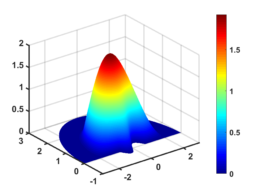
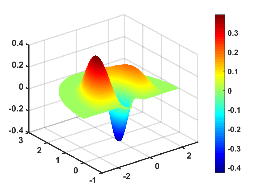
\displaystyle f(x,t):=\frac{e^{\frac{-|x-x_{0}|^{2}}{2\eta}}}{\sqrt{2\pi}\;\eta}\,\sin(2t),\;\eta=0.1,

where the excitation frequency is $\omega=2$ and the location of source is at $x_{0}=(0,0.5)$ . In Figure 3, we show the numerical solution at $t=2,4,8$ , respectively. It is observed that the waves are almost attenuated in the PML layer without reflections from the interface between the physical domain and PML layer.

To validate convergence of the PML method, we compute the relative error

\displaystyle E_{rel}:=\frac{\|u^{num}-u^{exa}\|_{L^{\infty}(0,T;L^{\infty}(\Omega_{\rho}^{+}))}}{\|u^{exa}\|_{L^{\infty}(0,T;L^{\infty}(\Omega_{\rho}^{+}))}},

where $u^{exa}$ represents the numerical solution with relatively larger absorbing parameters $\sigma$ , $\hat{\sigma}$ and with a larger thickness $\rho-R$ of the PML layer. Note that analytical solutions are not available in general.

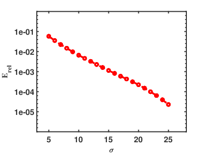
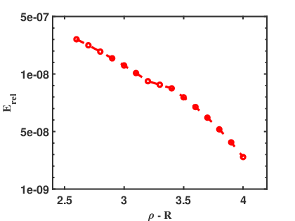
Figures 4 and 5 show the decaying behavior of the relative error $E_{rel}$ as the PML absorbing parameter $\sigma$ or the PML thickness $\rho-R$ increases. In Figure 4 we take the PML absorbing parameter $\sigma$ varying between $5$ and $25$ and fix the PML layer thickness at $\rho-R=1$ . Since the vertical axis is logarithmically scaled, the dashed lines indicate that the relative error $E_{rel}$ decays exponentially as $\sigma$ increases for a fixed layer thickness. In Figure 5 we display the relative error versus PML thickness $\rho-R$ for fixed absorbing $\sigma=25$ . We take the PML thickness $\rho-R$ ranging from $2.6$ to $4$ . It is obvious that relative error $E_{rel}$ decays exponentially as $\rho-R$ increases for a fixed absorbing parameter.

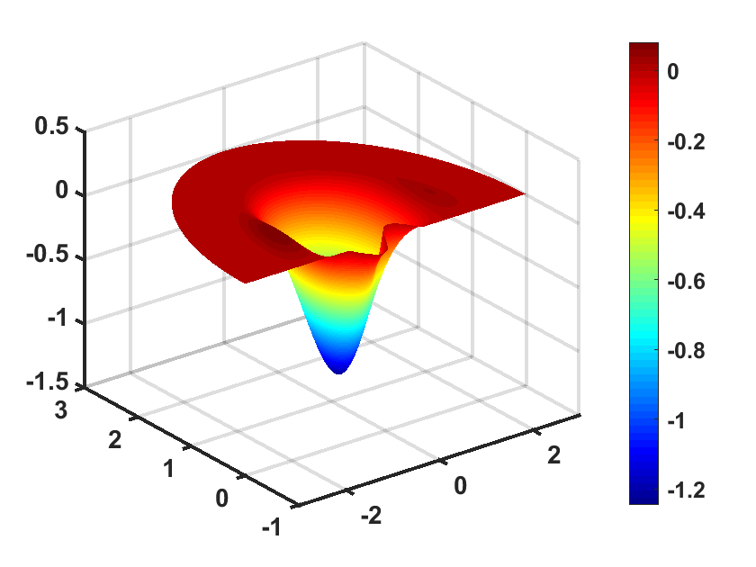
Example 2 In this example, we consider a non-harmonic source term, that is not compactly supported with respect to the time-variable. We take $R=2$ , $\rho=3.4$ and set $\sigma=\hat{\sigma}=25$ . A mesh of $11502$ vertices, $553$ edges and $22599$ triangles is applied and the final time is set at $t=10$ . The source is of the form

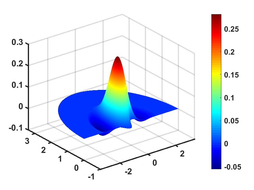
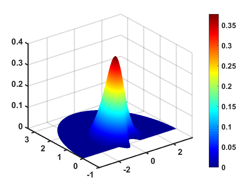
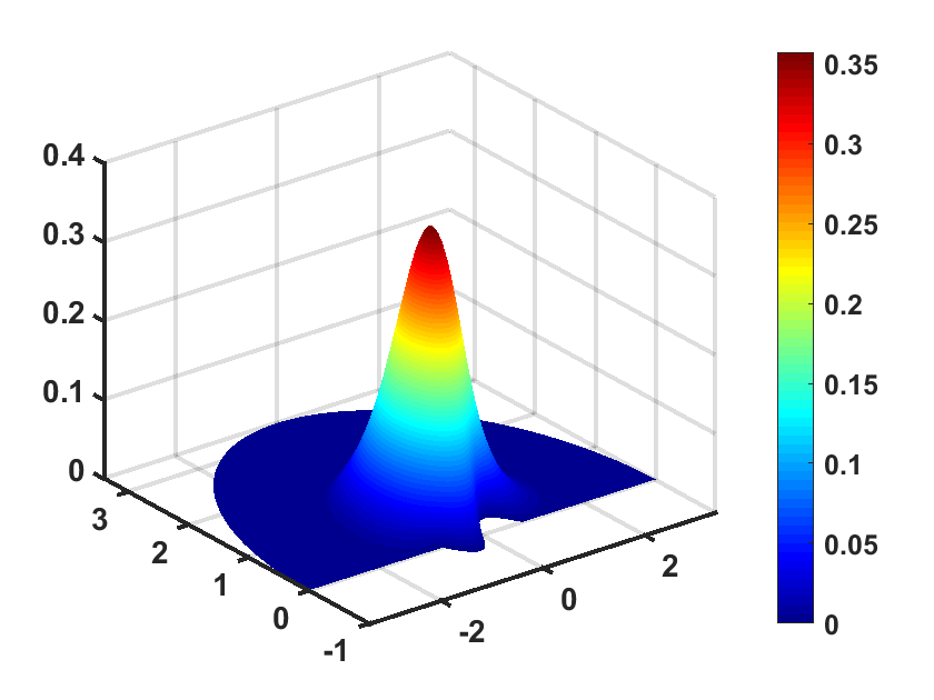
\displaystyle f(x,t):=\frac{e^{\frac{-|x-x_{0}|^{2}}{2\eta}}}{\sqrt{2\pi}\;\eta}\,t,\;\eta=0.1,

which is located at $(0,0.5)$ . We present in Figure 6 the numerical solutions at time $t=3,7,10$ , respectively. It shows that the source is excited all the time and rare reflection occurs at the interface $\Gamma_{R}^{+}$ .

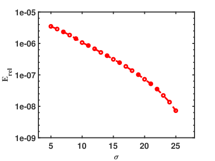
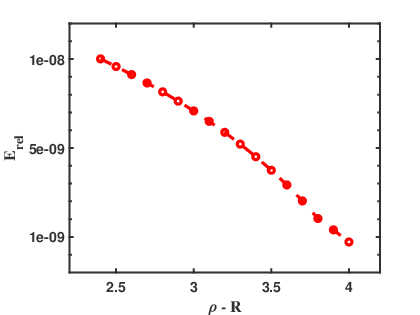
Figures 7 and 8 show the convergence of the relative error $E_{rel}$ versus one of the two PML parameters $\sigma$ and $\rho-R$ . In Figure 7, we present the relative error $E_{rel}$ versus the PML absorbing parameter $\sigma$ changing from $5$ to $25$ for the fixed PML thickness $\rho-R=1.4$ . As in Example 1, we observe that $E_{rel}$ decays exponentially as $\sigma$ increases. In Figure 8 we display the relative error versus the PML thickness $\rho-R$ for a fixed absorbing $\sigma=25$ . We take the PML thickness $\rho-R$ changing from $2.4$ to $4$ . It is obvious that the relative error $E_{rel}$ decays exponentially as $\rho-R$ increases.

6 Conclusion

In this paper we study the PML-method to the time domain acoustic scattering problem over a locally rough surface. We proved well-posedness of the scattering problem and the PML formulation. The long time stability of the PML formulations is obtained by the energy method. The exponential convergence of the PML solution is proved and it can be realized by either enlarging the PML absorbing parameter or the thickness of the layer. The convergence results are verified by two numerical examples.

Appendix A Laplace transform

For any $s=s_{1}+is_{2}$ with $s_{1}>0$ , $s_{2}\in{\mathbb{R}}$ , we define the Laplace transform of $u$ as

\displaystyle u_{L}(s)=\mathscr{L}(u)(s):=\int_{0}^{\infty}e^{-st}u(t)\,dt.

Some properties of the Laplace transform and its inversion are listed as follows:

$\displaystyle\mathscr{L}(\frac{du}{dt})$	$\displaystyle=$	$\displaystyle su_{L}-u(0),$	(A.1)
$\displaystyle\mathscr{L}(\frac{d^{2}u}{dt^{2}})$	$\displaystyle=$	$\displaystyle s^{2}u_{L}-su(0)-\frac{du}{dt}(0),$	(A.2)
$\displaystyle\int_{0}^{t}u(\tau)\,d\tau$	$\displaystyle=$	$\displaystyle\mathscr{L}^{-1}(s^{-1}u_{L}(s)).$	(A.3)

It can be verified from the inverse Laplace transform that

\displaystyle u(t)=\mathscr{F}^{-1}(e^{s_{1}t}\mathscr{L}(u)(s_{1}+is_{2})).

where $\mathscr{F}^{-1}$ denotes the inverse Fourier transform with respect to $s_{2}$ .

Below is the Parseval or Plancherel identity for the Laplace transform (see [22, equation (2.46)])

Lemma A.1.

(Parseval or Plancherel Identity) If $u_{L}=\mathscr{L}(u)$ and $v_{L}=\mathscr{L}(v)$ ,then

\displaystyle\frac{1}{2\pi}\int_{-\infty}^{+\infty}u_{L}(s)\,v_{L}(s)\,ds_{2}=\int_{0}^{\infty}e^{-2s_{1}t}u(t)\,v(t)\,dt,

(A.4)

for all $s_{1}>s_{0}$ , where $s_{0}$ is abscissa of convergence for Laplace transform of $u$ and $v$ .

The following lemma refers to [35, Theorem 43.1].

Lemma A.2.

let $\breve{\omega}(s)$ denote a holomorphic function in the half complex plane $\textnormal{Re}(s)>\sigma_{0}$ for some $\sigma_{0}\in{\mathbb{R}}$ , valued in the Banach space ${\mathcal{E}}$ . The following conditions are equivelent:

there is a distribution $\omega\in\mathcal{D}_{+}^{{}^{\prime}}$ whose Laplace transform is equal to $\breve{\omega}(s)$ , where $\mathcal{D}^{{}^{\prime}}_{+}({\mathcal{E}})$ is the space of distributions on the real line which vanish identically in the open negative half-line;

there is a $\sigma_{1}$ with $\sigma_{0}\leq\sigma_{1}<\infty$ and an integer $m\geq 0$ such that for all complex numbers $s$ with $\textnormal{Re}(s)>\sigma_{1}$ it holds that $\|\breve{\omega}(s)\|_{{\mathcal{E}}}\leq C(1+|s|)^{m}$ .

Appendix B Sobolev spaces

For a bounded domain $D$ with Lipschitz continuous boundary $\partial D$ , define the Sobolev space

\displaystyle H(\mbox{div},\,D):=\{u\in L^{2}(D):\nabla\cdot u\in L^{2}(D)\}.

which is a Hilbert space with the norm

\displaystyle\|u\|_{H(\mbox{div},\,D)}=\left(\|u\|^{2}_{L^{2}(D)}+\|\nabla\cdot u\|^{2}_{L^{2}(D)}\right)^{1/2}.

The first Green formula takes the form

\displaystyle(\nabla\cdot u,\,v)_{D}+(u,\,\nabla v)_{D}=\langle u\cdot n,\,v\rangle_{\partial D}\quad\mbox{for all}\quad u,v\in H(\mbox{div},\,D)

(B.1)

where $(\cdot,\cdot)_{D}$ and $\langle\cdot,\cdot\rangle_{\partial D}$ denote the $L^{2}$ -inner product on $D$ and the dual pairing product between $H^{-1/2}(\partial D)$ and $H^{1/2}(\partial D)$ , respectively.

Let $\Gamma_{R}^{+}$ be defined as in Section 2. For any $u\in C^{\infty}_{0}(\Gamma_{R}^{+})$ , we have the Fourier series expansion

\displaystyle u(R,\theta)=\sum_{n=1}^{\infty}a_{n}\sin n\theta,\quad a_{n}=\frac{2}{\pi}\int_{0}^{\pi}u(R,\theta)\sin n\theta\,d\theta.

Define the trace function space $H^{p}_{0}(\Gamma_{R}^{+})$ as

\displaystyle H^{p}_{0}(\Gamma_{R}^{+}):=\left\{u\in L^{2}(\Gamma_{R}^{+}):\|u\|_{H^{p}(\Gamma_{R}^{+})}:=\left(\sum_{n=1}^{\infty}(1+n^{2})^{p}|a_{n}|^{2}\right)^{1/2}<+\infty.\right\}.

Appendix C Modified Bessel functions

We look for solutions to the Helmholz equation

\displaystyle\Delta u(x)-s^{2}u(x)=0,

in the form of

\displaystyle u(x)=y(sr)e^{in\theta},\quad n=0,\pm 1,\pm 2,\cdots,

where $(r,\theta)$ are cylindrical coordinates. It is obvious that $y(r)$ is a solution of the ordinary equation

\displaystyle\frac{d^{2}y}{dr^{2}}+\frac{1}{r}\frac{dy}{dr}-\left(1+\frac{n^{2}}{r^{2}}\right)y=0.

The modified Bessel functions of order $\nu$ , which we denote by $K_{\nu}(z)$ , are solutions to the differential equation

\displaystyle z^{2}\frac{d^{2}y}{dz^{2}}+z\frac{dy}{dz}-(z^{2}+\nu^{2})y=0.

$K_{\nu}(z)$ satisfies the following asymptotic behavior as $|z|\rightarrow\infty$

\displaystyle K_{\nu}(z)\sim\left(\frac{\pi}{2z}\right)^{1/2}e^{-z}.

The following estimates for the modified Bessel function $K_{\nu}(z)$ have been proved in [19, Lemma 2.10 and 5.1] .

Lemma C.1.

Let $s=s_{1}+is_{2}$ with $s_{1}>0$ , $s_{2}\in{\mathbb{R}}$ . It holds that

\displaystyle-\textnormal{Re}\Big{(}\frac{K_{n}^{{}^{\prime}}(sR)}{K_{n}(sR)}\Big{)}\geq 0.

Lemma C.2.

Suppose $\nu\in{\mathbb{R}}$ , $s=s_{1}+is_{2}$ with $s_{1}>0$ , $s_{2}\in{\mathbb{R}}$ , $\rho_{1}>\rho_{2}>0$ and $\tau>0$ . It holds that

\displaystyle\frac{|K_{\nu}(s\rho_{1}+\tau)|}{|K_{\nu}(s\rho_{2})|}\leq e^{-\tau(1-\rho_{2}^{2}/\rho_{1}^{2})}.

Acknowledgements

G. Hu is partially supported by the National Natural Science Foundation of China (No. 12071236) and the Fundamental Research Funds for Central Universities in China (No. 63213025).

References

[1] H. Ammari, G. Bao, and A. Wood, An integral equation method for the electromagnetic scattering from cavities, Math. Methods Appl. Sci., 23 (2000), pp. 1057–1072.
[2] H. Ammari, G. Bao, and A. Wood, Analysis of the electromagnetic scattering from a cavity, Jpn. J. Ind. Appl. Math., 19 (2002), pp. 301–310.
[3] D. Appelo, T. Hagstrom, and G. Kreiss, Perfectly matched layers for hyperbolic systems: General formulation, well-posedness, and stability, SIAM J. Appl. Math., 67 (2006), pp. 1–23.
[4] G. Bao, and H. Wu, Convergence analysis of the PML problems for time-harmonic Maxwell’s equations, SIAM J. Numer. Anal., 43(2005), pp. 2121–2143.
[5] G. Bao, Y. Gao, and P. Li, Time-domain analysis of an acoustic-elastic interaction problem, Arch. Rational Mech. Anal., 229(2018), pp. 835–884.
[6] G. Bao, Y. Gao, and P. Li, Time-domain analysis of an acoustic-elastic interaction problem, Arch. Rational Mech. Anal. 229 (2018), PP. 835-884.
[7] J. P. Bérenger, A perfectly matched layer for the absorption of electromagnetic waves, J. Comput. Phys., 114(1994), pp. 185–200.
[8] J. P. Bérenger, Three-dimensional perfectly matched layer for the absorption of electromagnetic waves, J. Comput. Phys., 127(1996), pp. 363–379.
[9] E. Bécache, S. Fauqueux, and P. Joly, Stability of perfectly matched layers, group velocities and anisotropic waves, J. Comput. Phys., 188 (2003), pp. 399–433.
[10] E. Bécache and P. Joly, On the analysis of Bérenger’s perfectly matched layers for Maxwell equations, M2AN Math. Model. Numer. Anal., 36 (2002), pp. 87–119.
[11] E. Bécache and M. Kachanovska, Stability and convergence analysis of time-domain perfectly matched layers for the wave equation in waveguides, SIAM J. Numer. Anal. , 59(2021), pp.2004–2039.
[12] J. H. Bramble, and J. E. Pasciak, Analysis of a finite PML approximation for the three dimensional time-harmonic Maxwell and acoustic scattering problems, Math. Comp. 76 (2007), pp. 597–614.
[13] J. H. Bramble, and J. E. Pasciak, Analysis of a finite element PML approximation for the three dimensional time-harmonic Maxwell problem, Math. Comp., 77 (2008), pp. 1–10.
[14] J. H. Bramble, and J. E. Pasciak, Analysis of a Cartesian PML approximation to acoustic scattering problems in ${\mathbb{R}}^{2}$ and ${\mathbb{R}}^{3}$ , Math. Comp., 247 (2013), pp. 209-230.
[15] H. Brezis, Functional analysis, sobolev spaces and partial differential equations, Springer, 2010.
[16] W. Chew, and W. Weedon, A 3-D perfectly matched medium from modified Maxwell’s equation with stretched coordinates, Microw. Opt. Tech. Lett.,7(1994), pp. 599-604.
[17] Y. Chen, P. Li, and X. Yuan, An adaptive finite element PML method for the open cavity scattering problems, Commun. Comput. Phys., 29 (2021), pp. 1505-1540.
[18] Z. Chen, and W. Zheng, Convergence of the uniaxial perfectly matched layer method for time- harmonic scattering problems in two-layered media, SIAM J. Numer. Anal., 48 (2010), pp. 2158-2185.
[19] Z.Chen, Convergence of the time-domain perfectly matched layer method for acoustic scattering problems, International Journal of Numerical Analysis and Modeling, 6 (2009), pp. 124–146.
[20] Z. Chen, and X. Wu, Long-time stability and convergence of the uniaxial perfectly matched layer method for time-domain acoustic scattering problems, SIAM J. Numer. Anal. 50(2012), pp. 2632-2655.
[21] Z. Chen and J. Nedelec, On Maxwell equations with the transparent boundary condition, J. Comput. Math., 26(2008), pp. 284-296.
[22] A. M. Cohen, Numerical methods for Laplace Transform inversion, Numer. Methods Algorithms, 5, Springer, New York, 2007.
[23] F. Collino, and, P. Monk, The perfectly matched layer in curvilinear coordinates, SIAM J.Sci. Comput. 19(1998), pp. 1061–1090.
[24] J. Diaz, and, P. Joly, A time domain analysis of PML models in acoustics.Comput. Methods Appl. Mech. Eng. 195(2006), pp. 3820–3853.
[25] T. Hohage, F. Schmidt, and L. Zschiedrich, Solving time-harmonic scattering problems based on the pole condition II: Convergence of the PML method, SIAM J. Math. Anal., 35(2003), pp. 547-560.
[26] A. T. De Hoop, P. M. Van den Berg, and, R. F. Remis, Absorbing boundary conditions and perfectly matched layers-analytic time-domain performance analysis, IEEE Trans. Magn. 38(2002), 657–660.
[27] P. Joly, Variational methods for time-dependent wave propagation problems, Lecture Notes in Computational Science and Engineering, 31(2003), pp. 201–264.
[28] P. Joly, An elementary introduction to the construction and the analysis of perfectly matched layers for time domain wave propagation, SeMA Journal, 57(2012), pp. 5-48.
[29] M. Lassas, and E. Somersalo, On the existence and convergence of the solution of PML equations, Computing, 60 (1998), pp. 229-241.
[30] P. Li, A survey of open cavity scattering problems, J. Comp. Math., 36 (2018), pp. 1–16.
[31] P. Li, L. Wang, and A. Wood, Analysis of transient electromagnetic scattering from a three-dimensional open cavity, SIAM J. Appl. Math., 75(2015), pp. 1674-1699.
[32] J. L. Lions and E. Magenes, Non-Homogeneous Boundary Value Problems and Applications, Vol. I, Springer-Verlag, New York-Heidelberg, 1972.
[33] W. Mclean, Strongly elliptic system and boundary integral equations, Cambridge University Press, 2000.
[34] P. G. Petropoulos, Reflectionless sponge layers as absorbing boundary conditions forthe numerical solutions of Maxwellequation in Rectangular, cylindrical, and sopherical coordinates, SIAM J. Appl. Math., 60(2000), PP. 1037-1058.
[35] F. Tréves, Basic linear partial differential equations, Ann. of Math., 47(1975), pp. 202–212.
[36] E. Turkel, and, A. Yefet, Absorbing PML boundary layers for wave-like equations. Appl. Numer. Math. 27(1998), pp. 533–557.
[37] C. K. Wei, and J. Q. Yang, Analysis of a time-dependent fluid-solid interaction problem above a local rough surface, Sci China Math, 62 (2019).
[38] C. K. Wei, J. Q. Yang, and B. Zhang, Convergence analysis of the PML method for time-domain electromagnetic scattering problems, SIAM J. Numer. Anal, 58(2020), pp. 1918-1940.
[39] A. Wood, Analysis of electromagnetic scattering from an overfilled cavity in the ground plane, J.Comput. Phys., 215 (2006), pp. 630–641.

	$\displaystyle\Big{\|}\langle\mathscr{G}(\omega),\,\phi\rangle_{\Gamma_{R}^{+}}\Big{\|}$	$\displaystyle=\Big{\|}\int_{\Gamma_{R}^{+}}s\sum_{n=1}^{\infty}\frac{K_{n}^{{}^{\prime}}(sR)}{K_{n}(sR)}\omega_{n}(R)\sin n\theta\sum_{n=1}^{\infty}\overline{\phi}_{n}(R)\sin n\theta\,d\gamma\Big{\|}$
		$\displaystyle=\Big{\|}sR\sum_{n=1}^{\infty}\frac{K_{n}^{{}^{\prime}}(sR)}{K_{n}(sR)}\omega_{n}(R)\overline{\phi}_{n}(R)\int_{0}^{\pi}\sin^{2}n\theta\,d\theta$
		$\displaystyle=\Big{\|}\frac{\pi}{2}sR\sum_{n=1}^{\infty}\frac{K_{n}^{{}^{\prime}}(sR)}{K_{n}(sR)}\omega_{n}(R)\overline{\phi}_{n}(R)\Big{\|}$
		$\displaystyle\leq\frac{\pi}{2}\|s\|R\Big{(}\sum_{n=1}^{\infty}\Big{\|}\frac{K_{n}^{{}^{\prime}}(sR)}{K_{n}(sR)}\Big{\|}\|\omega_{n}(R)\|^{2}\Big{)}^{1/2}\Big{(}\sum_{n=1}^{\infty}\Big{\|}\frac{K_{n}^{{}^{\prime}}(sR)}{K_{n}(sR)}\Big{\|}\|\phi_{n}(R)\|^{2}\Big{)}^{1/2}$
		$\displaystyle\leq C\Big{(}\sum_{n=1}^{\infty}\sqrt{1+n^{2}}\|\omega_{n}(R)\|^{2}\Big{)}^{1/2}\Big{(}\sum_{n=1}^{\infty}\sqrt{1+n^{2}}\|\phi_{n}(R)\|^{2}\Big{)}^{1/2}$
		$\displaystyle\leq C\\|\omega\\|_{H^{1/2}_{0}(\Gamma_{R}^{+})}\,\\|\phi\\|_{H^{1/2}_{0}(\Gamma_{R}^{+})}.$

$\displaystyle\|a(u_{L},\,v)\|$	$\displaystyle\leq$	$\displaystyle\|s\|^{-1}\\|\nabla u_{L}\\|_{L^{2}(\Omega_{R}^{+})}\\|\nabla v\\|_{L^{2}(\Omega_{R}^{+})}+\|s\|\\|u_{L}\\|_{L^{2}(\Omega_{R}^{+})}\\|v\\|_{L^{2}(\Omega_{R}^{+})}$
		$\displaystyle+\|s\|^{-1}\\|\mathscr{G}u_{L}\\|_{H^{-1/2}(\Gamma_{R}^{+})}\\|v\\|_{H^{1/2}(\Gamma_{R}^{+})}$
	$\displaystyle\leq$	$\displaystyle C\\|u_{L}\\|_{H^{1}(\Omega_{R}^{+})}\\|v\\|_{H^{1}(\Omega_{R}^{+})}+C\\|u_{L}\\|_{H^{1}(\Omega_{R}^{+})}\\|v\\|_{H^{1}(\Omega_{R}^{+})}$
		$\displaystyle C\\|u_{L}\\|_{H^{1/2}(\Gamma_{R}^{+})}\\|v\\|_{H^{1/2}(\Gamma_{R}^{+})}$
	$\displaystyle\leq$	$\displaystyle C\\|u_{L}\\|_{H^{1}(\Omega_{R}^{+})}\\|v\\|_{H^{1}(\Omega_{R}^{+})}.$

	$\displaystyle\\|\nabla u_{L}\\|_{L^{2}(\Omega_{R}^{+})}+\\|su_{L}\\|_{L^{2}(\Omega_{R}^{+})}$	$\displaystyle\leq$	$\displaystyle\left(\\|\nabla u_{L}\\|_{L^{2}(\Omega_{R}^{+})}^{2}+\\|su_{L}\\|_{L^{2}(\Omega_{R}^{+})}^{2}\right)^{1/2}$
		$\displaystyle\leq$	$\displaystyle C\frac{(1+\|s\|)\|s\|}{s_{1}}\\|f_{L}\\|_{L^{2}(\Omega_{R}^{+})},$

			$\displaystyle\int_{0}^{\infty}e^{-2s_{1}t}(\\|\partial_{t}u\\|_{L^{2}(\Omega_{R}^{+})}^{2}+\\|\nabla u\\|_{L^{2}(\Omega_{R}^{+})}^{2})\,dt$
	$\displaystyle=$		$\displaystyle\frac{1}{2\pi}\int_{-\infty}^{+\infty}\\|su_{L}\\|_{L^{2}(\Omega_{R}^{+}}^{2}+\\|\nabla u_{L}\\|_{L^{2}(\Omega_{R}^{+})}^{2})\,ds_{2}$
	$\displaystyle\leq$		$\displaystyle C\frac{1}{s_{1}^{2}}\int_{-\infty}^{+\infty}(1+\|s\|)^{2}\|s\|^{2}\\|f_{L}\\|_{L^{2}(\Omega_{R}^{+})}^{2}\,ds_{2}$
	$\displaystyle\leq$		$\displaystyle C\frac{1}{s_{1}^{2}}\int_{-\infty}^{+\infty}\\|s^{2}f_{L}\\|_{L^{2}(\Omega_{R}^{+})}^{2}+\\|sf_{L}\\|_{L^{2}(\Omega_{R}^{+})}^{2}\,ds_{2}$
	$\displaystyle\leq$		$\displaystyle C\frac{1}{s_{1}^{2}}\int_{0}^{\infty}e^{-2s_{1}t}\left(\\|\partial_{t}^{2}f\\|_{L^{2}(\Omega_{R}^{+})}^{2}+\\|\partial_{t}f\\|_{L^{2}(\Omega_{R}^{+})}^{2}\right)\,dt.$

			$\displaystyle\max_{0\leq t\leq T}\Big{(}\\|\partial_{t}u\\|_{L^{2}(\Omega_{R}^{+})}+\\|\nabla u\\|_{L^{2}(\Omega_{R}^{+})}\Big{)}$
	$\displaystyle\leq$		$\displaystyle C\max_{0\leq t\leq T}\Big{(}\\|\partial_{t}u\\|_{L^{2}(\Omega_{R}^{+})}^{2}+\\|\nabla u\\|_{L^{2}(\Omega_{R}^{+})}^{2}\Big{)}^{1/2}$
	$\displaystyle\leq$		$\displaystyle C\\|\partial_{t}f\\|_{L^{1}(0,T;L^{2}(\Omega_{R}^{+}))}.$