This paper was converted on www.awesomepapers.org from LaTeX by an anonymous user.
Want to know more? Visit the Converter page.

\RS@ifundefined

subsecref \newrefsubsecname = \RSsectxt \RS@ifundefinedthmref \newrefthmname = theorem  \RS@ifundefinedlemref \newreflemname = lemma  \newrefthmname=Theorem ,Name=Theorem  \newrefpropname=Proposition ,Name=Proposition  \newrefdefname=Definition ,Name=Definition  \newreflemname=Lemma ,Name=Lemma  \newrefcorname=Corollary ,Name=Corollary  \newrefasmname=Assumption ,Name=Assumption  \newrefappname=Appendix ,Name=Appendix  \newrefclaimname=Claim ,Name=Claim 

Well-conditioned Primal-Dual Interior-point Method for Accurate Low-rank Semidefinite Programmingthanks: Financial support for this work was provided by NSF CAREER Award ECCS-2047462 and ONR Award N00014-24-1-2671.

Hong-Ming Chiu
University of Illinois Urbana-Champaign
[email protected]
   Richard Y. Zhang
University of Illinois Urbana-Champaign
[email protected]
Abstract

We describe how the low-rank structure in an SDP can be exploited to reduce the per-iteration cost of a convex primal-dual interior-point method down to O(n3)O(n^{3}) time and O(n2)O(n^{2}) memory, even at very high accuracies. A traditional difficulty is the dense Newton subproblem at each iteration, which becomes progressively ill-conditioned as progress is made towards the solution. Preconditioners have been proposed to improve conditioning, but these can be expensive to set up, and fundamentally become ineffective at high accuracies, as the preconditioner itself becomes increasingly ill-conditioned. Instead, we present a well-conditioned reformulation of the Newton subproblem that is cheap to set up, and whose condition number is guaranteed to remain bounded over all iterations of the interior-point method. In theory, applying an inner iterative method to the reformulation reduces the per-iteration cost of the outer interior-point method to O(n3)O(n^{3}) time and O(n2)O(n^{2}) memory. We also present a well-conditioned preconditioner that theoretically increases the outer per-iteration cost to O(n3r3)O(n^{3}r^{3}) time and O(n2r2)O(n^{2}r^{2}) memory, where rr is an upper-bound on the solution rank, but in practice greatly improves the convergence of the inner iterations.

1 Introduction

Given problem data 𝒜:𝒮nm\mathcal{A}:\mathcal{S}^{n}\to\mathbb{R}^{m} and bmb\in\mathbb{R}^{m} and C𝒮nC\in\mathcal{S}^{n}, we seek to solve the standard-form semidefinite program (SDP)

X\displaystyle X^{\star} =argminX𝒮n{C,X:𝒜(X)=b,X0},\displaystyle=\arg\min_{X\in\mathcal{S}^{n}}\{\left\langle C,X\right\rangle:\mathcal{A}(X)=b,\quad X\succeq 0\}, (1a)
y,S\displaystyle y^{\star},S^{\star} =argmaxS𝒮n,ym{b,y:𝒜T(y)+S=C,S0},\displaystyle=\arg\max_{S\in\mathcal{S}^{n},y\in\mathbb{R}^{m}}\{\left\langle b,y\right\rangle:\mathcal{A}^{T}(y)+S=C,\quad S\succeq 0\}, (1b)
assuming that the primal problem (1a) admits a unique low-rank solution
X is unique, r=defrank(X)n,X^{\star}\text{ is unique, }\quad r^{\star}\overset{\mathrm{def}}{=}\mathrm{rank}\,(X^{\star})\ll n, (1c)
and that the dual problem (1b) admits a strictly complementary solution (not necessarily unique)
exists S such that rank(S)=nr.\text{exists }S^{\star}\text{ such that }\mathrm{rank}\,(S^{\star})=n-r^{\star}. (1d)

Here, 𝒮n\mathcal{S}^{n} denotes the space of n×nn\times n real symmetric matrices with the inner product A,B=tr(AB)\langle A,B\rangle=\operatorname{tr}(AB), and ABA\succeq B signifies that ABA-B is positive semidefinite. We assume without loss of generality that the constraints represented by 𝒜\mathcal{A} are linearly independent, meaning 𝒜T(y)=0\mathcal{A}^{T}(y)=0 implies y=0y=0. This assumption restricts the number of constraints to m12n(n+1)m\leq\frac{1}{2}n(n+1). Both of these conditions are mild and are widely regarded as standard assumptions.

Currently, the low-rank SDP (1) is most commonly approached using the nonconvex Burer–Monteiro factorization [12], which is to factorize X=UUTX=UU^{T} into an n×rn\times r low-rank factor UU, where rrr\geq r^{\star} is a search rank parameter, and then to locally optimize over UU. While this can greatly reduce the number of optimization variables, from O(n2)O(n^{2}) down to as low as O(n)O(n), the loss of convexity can create significant convergence difficulties. A basic but fundamental issue is the possibility of failure by getting stuck at a spurious local minimum over the low-rank factor UU [11]. Even ignoring this potential failure mode, it can still take a second-order method like cubic regularization or a trust-region method up to O(ϵ3/2)O(\epsilon^{-3/2}) iterations to reach ϵ\epsilon second-order optimality over UU, where a primal-solution (X,y,S)(X,y,S) with ϵ\epsilon duality gap can (hopefully) be extracted [11]. In practice, the Burer–Monteiro approach works well for some problems [10, 38, 20], but as shown in Fig. 1, can be slow and unreliable for other problems, particularly those with underlying nonsmoothness.

Refer to caption
Figure 1: Error XXF\|X-X^{\star}\|_{F} against runtime for solving trace-regularized linear regression as an instance of (1) using our proposed method (Our method); spectrally preconditioned interior-point method by Zhang and Lavaei [53] (ZL17); the Burer-Monteiro method, implemented with nonlinear programming solvers Fmincon [33] and Knitro [13], and equipped with analytic Hessians; alternating direction method of multipliers (ADMM); and subgradient method (SubGD). (See Section 7.2 for details.)

In this paper, we revisit classical primal-dual interior-point methods (IPMs), because they maintain the convexity of the SDP (1), and therefore enjoy simple and rapid global convergence to ϵ\epsilon duality gap in O(nlog(1/ϵ))O(\sqrt{n}\log(1/\epsilon)) iterations. IPMs are second-order methods that solve a sequence of logarithmic penalized SDPs of the form

X(μ)\displaystyle X(\mu) =argminX𝒮n{C,Xμlogdet(X):𝒜(X)=b},\displaystyle=\arg\min_{X\in\mathcal{S}^{n}}\{\left\langle C,X\right\rangle-\mu\log\det(X):\mathcal{A}(X)=b\},
y(μ),S(μ)\displaystyle y(\mu),S(\mu) =argmaxS𝒮n,ym{b,y+μlogdet(S):𝒜T(y)+S=C},\displaystyle=\arg\max_{S\in\mathcal{S}^{n},y\in\mathbb{R}^{m}}\{\left\langle b,y\right\rangle+\mu\log\det(S):\mathcal{A}^{T}(y)+S=C\},

while progressively decreasing the duality gap parameter μ>0\mu>0 after each iteration. Using an IPM, the cost of solving (1) is almost completely determined by the cost of solving the Newton subproblem at each iteration

minΔX𝒮n{C~,ΔX+12W1/2(ΔX)W1/2F2:𝒜(ΔX)=b~},\displaystyle\min_{\Delta X\in\mathcal{S}^{n}}\left\{\left\langle\tilde{C},\Delta X\right\rangle+\frac{1}{2}\|W^{-1/2}(\Delta X)W^{-1/2}\|_{F}^{2}:\mathcal{A}(\Delta X)=\tilde{b}\right\}, (2a)
maxΔS𝒮n,Δym{b~,Δy12W1/2(ΔS)W1/2F2:𝒜T(Δy)+ΔS=C~},\displaystyle\max_{\Delta S\in\mathcal{S}^{n},\Delta y\in\mathbb{R}^{m}}\left\{\left\langle\tilde{b},\Delta y\right\rangle-\frac{1}{2}\|W^{1/2}(\Delta S)W^{1/2}\|_{F}^{2}:\mathcal{A}^{T}(\Delta y)+\Delta S=\tilde{C}\right\}, (2b)
in which the scaling point W𝒮++nW\in\mathcal{S}_{++}^{n} and the residuals b~m,C~𝒮n\tilde{b}\in\mathbb{R}^{m},\tilde{C}\in\mathcal{S}^{n} are iteration- and algorithm-dependent. In fact, using a short-step strategy (with fixed step-sizes) [36, Theorem 6.1], solving the SDP (1) to ϵ\epsilon duality gap costs exactly the same as solving an instances of (2) to ϵ\epsilon accuracy. By paying some small per-iteration overhead, long-step strategies (with adaptive step-sizes) can consistently reduce the iteration count down to 50-100 in practice [47, 42].

Instead, the traditional difficulty faced by IPMs is the high cost of accurately solving the Newton subproblem (2) at each iteration. This difficulty arises due to need to use a scaling point W𝒮++nW\in\mathcal{S}_{++}^{n} that is both dense and becomes increasing ill-conditioned with decreasing values of μ\mu. Although our technique is more broadly applicable, we will focus this paper on the primal-dual Nesterov–Todd scaling [35, 36], which is computed from the current iterates X,SX,S as follows

W=X1/2(X1/2SX1/2)1/2X1/2=[S1/2(S1/2XS1/2)1/2S1/2]1,W=X^{1/2}(X^{1/2}SX^{1/2})^{-1/2}X^{1/2}=[S^{1/2}(S^{1/2}XS^{1/2})^{-1/2}S^{1/2}]^{-1}, (2c)

and appears in popular general-purpose IPM solvers like SeDuMi [41], SDPT3 [46], and MOSEK [34]. The ill-conditioning in WW makes it increasingly difficult to solve (2) to sufficiently high accuracy for the outer IPM to continue making progress. Therefore, most IPM solvers, like those listed above, solve (2) by directly forming and factorizing its Karush–Kuhn–Tucker equations. Unfortunately, the density of WW renders these equations dense, irrespective of any sparsity in the data CC and 𝒜\mathcal{A}. For SDPs with m=Θ(n2)m=\Theta(n^{2}) constraints, the cost of solving (2) by the direct approach is Θ(n6)\Theta(n^{6}) time and Θ(n4)\Theta(n^{4}) memory, hence limiting nn to no more than about 200.

In this paper, we instead solve (2) using a preconditioned iterative approach, as a set of inner iterations within the outer IPM iterations. Our main contribution is to use the low-rank structure in (1) to provably reduce the cost of computing a numerically exact solution to (2) to O(n3r3log(1/εmach)))O(n^{3}r^{3}\log(1/\varepsilon_{\mathrm{mach}}))) time and O(n2r2)O(n^{2}r^{2}) memory, where rrr\geq r^{\star} is a search rank parameter as before, and εmach\varepsilon_{\mathrm{mach}} is the machine precision. Critically, these complexity figures hold even for SDPs with m=Θ(n2)m=\Theta(n^{2}) constraints. This matches the per-iteration costs of second-order implementations of the Burer–Monteiro method, but we additionally retain the O(nlog(1/ϵ))O(\sqrt{n}\log(1/\epsilon)) iteration bound enjoyed by classical IPMs. As we now explain, our main challenge is being able to maintain these complexity figures even at high accuracies, where μ\mu becomes very small, and WW becomes extremely ill-conditioned.

1.1 Prior work: Spectral preconditioning

By taking advantage of fast matrix-vector products with the data 𝒜\mathcal{A}, an iterative approach can reduce the cost of solving the Newton subproblem (2) to as low as O(n3)O(n^{3}) time and O(n2)O(n^{2}) memory. However, without an effective preconditioner, these improved complexity figures are limited to coarse accuracies of μ102\mu\approx 10^{-2}. The key issue is that the scaling point WW becomes ill-conditioned as cond(W)=Θ(1/μ)\operatorname{cond}(W)=\Theta(1/\mu). Iterating until the numerical floor yields a numerically exact solution to (2) that is indistinguishable from the true solution under finite precision, but the number of iterations to achieve this grows as O(1/μlog(1/εmach))O(1/\mu\log(1/\varepsilon_{\mathrm{mach}})). Truncating after a much smaller number of iterations yields an inexact solution to (2) that can slow the convergence of the outer IPM.

Toh and Kojima [45] proposed the first effective preconditioner for SDPs. Their critical insight is the empirical observation that the scaling point W𝒮++nW\in\mathcal{S}_{++}^{n} becomes ill-conditioned as cond(W)=Θ(1/μ)\operatorname{cond}(W)=\Theta(1/\mu) only because its eigenvalues split into two well-conditioned clusters:

W=QΛQTtop r eigenvalues+QΛQT,bottom nr eigenvalueswhere Λ=Θ(1/μ) and Λ=Θ(μ).W=\underbrace{Q\Lambda Q^{T}}_{\text{top }r^{\star}\text{ eigenvalues}}+\underbrace{Q_{\perp}\Lambda_{\perp}Q_{\perp}^{T},}_{\text{bottom }n-r^{\star}\text{ eigenvalues}}\,\text{where }\Lambda=\Theta(1/\sqrt{\mu})\text{ and }\Lambda_{\perp}=\Theta(\sqrt{\mu}). (A0)

Based on this insight, they formulated a spectral preconditioner that attempts to counteract the ill-conditioning between the two clusters, and demonstrated promising computational results. However, the empirical effectiveness was not rigorously guaranteed, and its expensive setup cost of O(mn3)O(mn^{3}) time made its overall solution time comparable to a direct solution of (2), particularly for problems with m=Θ(n2)m=\Theta(n^{2}) constraints.

Inspired by the above, Zhang and Lavaei [53] proposed a spectral preconditioner that is much cheaper to set up, and also rigorously guarantees a high quality of preconditioning under the splitting assumption (A0). Their key idea is to rewrite the scaling point as the low-rank perturbation of a well-conditioned matrix, and then to approximate the well-conditioned part by the identity matrix

W=Q(Λτ)QTlow-rank+τ(QQT+τ1QΛQT)well-conditionedUUT+τI.W=\quad\underbrace{Q(\Lambda-\tau)Q^{T}}_{\text{low-rank}}\quad+\quad\tau\cdot\underbrace{(QQ^{T}+\tau^{-1}Q_{\perp}\Lambda_{\perp}Q_{\perp}^{T})}_{\text{well-conditioned}}\quad\approx\quad UU^{T}\quad+\quad\tau I.

Indeed, it is easy to verify that the joint condition number between WW and UUT+τIUU^{T}+\tau I is bounded under (A0) even as μ0+\mu\to 0^{+}. Substituting WUUT+τIW\approx UU^{T}+\tau I into (2) reveals a low-rank perturbed problem that admits a closed-form solution via the Sherman–Morrison–Woodbury formula, which they proposed to use as a preconditioner. Assuming (A0) and the availability of fast matrix-vector products that we outline as (A3) below, they proved that their method computes a numerically exact solution in O(n3r3+n3r2log(1/εmach))O(n^{3}r^{3}+n^{3}r^{2}\log(1/\varepsilon_{\mathrm{mach}})) time and O(n2r2)O(n^{2}r^{2}) memory. This same preconditioning idea was later adopted in the solver Loraine [27].

In practice, however, the Zhang–Lavaei preconditioner loses its effectiveness for smaller values of μ\mu, until abruptly failing at around μ106\mu\approx 10^{-6}. This is an inherent limitation of preconditioning in finite-precision arithmetic; to precondition a matrix with a diverging condition number Θ(1/μ2)\Theta(1/\mu^{2}), the preconditioner’s condition number must also diverge as Θ(1/μ2)\Theta(1/\mu^{2}). As μ\mu approaches zero, it eventually becomes impossible to solve the preconditioner accurately enough for it to remain effective. This issue is further exacerbated by the use of the Sherman–Morrison–Woodbury formula, which is itself notorious for numerical instability.

Moreover, the effectiveness of both prior preconditioners critically hinges on the splitting assumption (A0), which lacks a rigorous justification. It was informally argued in [45, 44] that the assumpution holds under strict complementarity (1d) and the primal-dual nondegeneracy of Alizadeh, Haeberly, and Overton [2]. But primal-dual nondegeneracy is an excessively strong assumption, as it would require the number of constraints mm to be within the range of

12r(r+1)mnr12r(r1).\frac{1}{2}r^{\star}(r^{\star}+1)\leq m\leq nr^{\star}-\frac{1}{2}r^{\star}(r^{\star}-1).

In particular, it is not applicable to the diverse range of low-rank matrix recovery problems, like matrix sensing [37, 17], matrix completion [15], phase retrieval [18], that necessarily require m>nr12r(r1)m>nr^{\star}-\frac{1}{2}r^{\star}(r^{\star}-1) measurements in order to uniquely recover an underlying rank-rr^{\star} ground truth. It is also not applicable to problems with m=Θ(n2)m=\Theta(n^{2}) constraints, which as we explained above, are the most difficult SDPs to solve for a fixed value of nn.

1.2 This work: Well-conditioned reformulation and preconditioner

In this paper, we derive a well-conditioned reformulation of the Newton subproblem (2) that costs just O(n3)O(n^{3}) time and O(n2)O(n^{2}) memory to set up. In principle, as the reformulation is already well-conditioned by construction, it allows any iterative method to compute a numerically exact solution in O(log(1/εmach))O(\log(1/\varepsilon_{\mathrm{mach}})) iterations for all values of 0<μ10<\mu\leq 1. In practice, the convergence rate can be substantially improved by the use of a well-conditioned preconditioner. Assuming (A0) and the fast matrix-vector products in (A3) below, we provably compute a numerically exact solution in O(n3r3+n3r2log(1/εmach))O(n^{3}r^{3}+n^{3}r^{2}\log(1/\varepsilon_{\mathrm{mach}})) time and O(n2r2)O(n^{2}r^{2}) memory. But unlike Zhang and Lavaei [53], our well-conditioned preconditioner maintains its full effectiveness even at extremely high accuracies like μ1012\mu\approx 10^{-12}, hence fully addressing a critical weakness of this prior work.

Our main theoretical results are a tight upper bound on the condition number of the reformulation and the preconditioner (3.3), and a tight bound on the number of preconditioned iterations needed to solve (2) to ϵ\epsilon accuracy (3.5). These rely on the same splitting assumption (A0) as prior work, which we show is implied by a strengthened version of strict complementarity (1d). In 3.1, we prove that (A0) holds if the primal-dual iterates (X,S)(X,S) used to compute the scaling point WW in (2) satisfy the following centering condition (the spectral norm \|\cdot\| is defined as the maximum singular value):

1μX1/2SX1/2I<1,XX=O(μ),SS=O(1).\left\|\frac{1}{\mu}X^{1/2}SX^{1/2}-I\right\|<1,\qquad\|X-X^{\star}\|=O(\mu),\qquad\|S-S^{\star}\|=O(1). (A1)

In particular, the restrictive primal-dual nondegeneracy assumption adopted by prior work [45, 44] is completely unnecessary. By repeating the algebraic derivations in [30], it can be shown that (A1) holds under strict complementarity (1d) if the IPM maintains its primal-dual iterates (X,S)(X,S) within the “wide” neighborhood 𝒩\mathcal{N}_{\infty} [48, 35, 6]. In turn, most IPMs that achieve an ϵ\epsilon duality gap in O(nlog(1/ϵ))O(\sqrt{n}\log(1/\epsilon)) iterations—including essentially all theoretical short-step methods [35, 36, 43] but also many practical methods like the popular solver SeDuMi [41]—do so by keeping their iterates within the 𝒩\mathcal{N}_{\infty} neighborhood [42]. In Section 7.1, we experimentally verify for SDPs satisfying strict complementarity (1d) that SeDuMi [41] keeps its primal-dual iterates (X,S)(X,S) sufficiently centered to satisfy (A1).

Under (A1), which implies the splitting assumption (A0) adopted in prior work via 3.1, we prove that O(log(1/ϵ))O(\log(1/\epsilon)) preconditioned iterations solve (2) to ϵ\epsilon accuracy for all values of 0<μ10<\mu\leq 1. In order for the reformulation and the preconditioner to remain well-conditioned, however, we require a strengthened version of the primal uniqueness assumption (1c). Concretely, we require the linear operator 𝒜\mathcal{A} to be injective with respect to the tangent space of the manifold of rank-rr^{\star} positive semidefinite matrices, evaluated at the unique primal solution X=UUTX^{\star}=U^{\star}U^{\star T}:

𝒜(UVT+VUT)=0UVT+VUT=0.\displaystyle\mathcal{A}(U^{\star}V^{T}+VU^{\star T})=0\quad\iff\quad U^{\star}V^{T}+VU^{\star T}=0. (A2)

This is stronger than primal uniqueness because it is possible for a rank-rr^{\star} primal solution to be unique with just m=12r(r+1)m=\frac{1}{2}r^{\star}(r^{\star}+1) constraints [2], but (A2) can hold only when the number of constraints mm is no less than the dimension of the tangent space

m12r(r+1)+r(nr)=nr12r(r1).m\geq\frac{1}{2}r^{\star}(r^{\star}+1)+r^{\star}(n-r^{\star})=nr^{\star}-\frac{1}{2}r^{\star}(r^{\star}-1).

Fortunately, many rigorous proofs of primal uniqueness, such as for matrix sensing [37, 17], matrix completion [15], phase retrieval [18], actually work by establishing (A2). In problems where (A2) does not hold, it becomes possible for our reformulation and preconditioner to grow ill-conditioned in the limit μ0+\mu\to 0^{+}. For these cases, the behavior of our method matches that of Zhang and Lavaei [53]; down to modest accuracies of μ106\mu\approx 10^{-6}, our preconditioned iterations will still rapidly converge to ϵ\epsilon accuracy in O(log(1/ϵ))O(\log(1/\epsilon)) iterations.

Our time complexity figures require the same fast matrix-vector products as previously adopted by Zhang and Lavaei [53] (and implicitly adopted by Toh and Kojima [45]). We assume, for U,Vn×rU,V\in\mathbb{R}^{n\times r} and ymy\in\mathbb{R}^{m}, that the two matrix-vector products

𝒜(UVT+VUT)=[Ai,UVT+VUT]i=1m,𝒜T(y)U=i=1myiAiU\mathcal{A}(UV^{T}+VU^{T})=\left[\left\langle A_{i},UV^{T}+VU^{T}\right\rangle\right]_{i=1}^{m},\quad\mathcal{A}^{T}(y)U=\sum_{i=1}^{m}y_{i}A_{i}U (A3)

can both be performed in O(n2r)O(n^{2}r) time and O(n2)O(n^{2}) storage. This is satisfied in problems with suitable sparsity and/or Kronecker structure. In Section 7.1, we rigorously prove that the robust matrix completion and sensor network localization problems satisfy (A3) due to suitable sparsity in the operator 𝒜\mathcal{A}.

1.3 Related work

Our well-conditioned reformulation of the Newton subproblem (2) is inspired by Toh [44] and shares superficial similarities. Indeed, the relationship between our reformulation and the Zhang–Lavaei preconditioner [53] has an analogous relationship to Toh’s reformulation with respect to the Toh–Kojima preconditioner [45]. However, the actual methods are very different. First, Toh’s reformulation remains well-conditioned only under primal-dual nondegeneracy, which as we explained above, makes it inapplicable to most low-rank matrix recovery problems, as well as problems with m=Θ(n2)m=\Theta(n^{2}) constraints. Second, the effectiveness of Toh’s preconditioner is not rigorously guaranteed; due to its reliance on the PSQMR method, the Faber–Manteuffel Theorem [22] says that it is fundamentally impossible to prove convergence for the preconditioned iterative method. Third, our set-up cost of O(n3r3)O(n^{3}r^{3}) is much cheaper than Toh’s set-up cost of O(mn3)O(mn^{3}); this parallels the reduction in set-up cost achieved by the Zhang–Lavaei preconditioner [53] over the Toh–Kojima preconditioner [45].

We mention another important line of work on the use of partial Cholesky preconditioners [7, 24, 4], which was extended to IPMs for SDPs in [5]. These preconditioners are based on the insight that a small number of ill-conditioned dimensions in the Newton subproblem (2) can be corrected by a low-rank partial Cholesky factorization of its underlying Schur complement. However, to the best of our knowledge, such preconditioners do not come with rigorous guarantees of an improvement.

Outside of SDPs, our reformulation is also inspired by the layered least-squares of Bobrovnikova and Vavasis [9]; indeed, our method can be viewed as the natural SDP generalization. However, an important distinction is that they apply MINRES directly to solve the indefinite reformulation, whereas we combine PCG with an indefinite preconditioner to dramatically improve the convergence rate. This idea of using PCG to solve indefinite equations with an indefinite preconditioner had first appeared in the scientific computing literature [29, 25, 39].

We mention that first-order methods have also been derived to exploit the low-rank structure of the SDP (1) without giving up the convexity [14, 51, 49]. These methods gain their efficiency by keeping all their iterates low-rank, and by performing convex updates on the low-rank iterates X=UUTX=UU^{T} while maintaining them in low-rank factored form X+=U+U+TX_{+}=U_{+}U_{+}^{T}. While convex first-order methods cannot become stuck at a spurious local minimum, they still require poly(1/ϵ)\mathrm{poly}(1/\epsilon) iterations to converge to an ϵ\epsilon-accurate solution of (1). In contrast, our proposed method achieves the same in just O(log(1/ϵ))O(\log(1/\epsilon)) iterations, for an exponential factor improvement.

Finally, for low-rank SDPs with small treewidth sparsity, chordal conversion methods [23, 28] compute an ϵ\epsilon accurate solution in guaranteed O(n1.5log(1/ϵ))O(n^{1.5}\log(1/\epsilon)) time and O(n)O(n) memory [54, 52]. Where the property holds, chordal conversion methods achieve state-of-the-art speed and reliability. Unfortunately, many real-world problems do not enjoy small treewidth sparsity [32]. For low-rank SDPs that are sparse but non-chordal, our proposed method can solve them in as little as O(n3.5log(1/ϵ))O(n^{3.5}\log(1/\epsilon)) time and O(n2)O(n^{2}) memory.

Notations

Write n×n𝒮n𝒮+n𝒮++n\mathbb{R}^{n\times n}\supseteq\mathcal{S}^{n}\supseteq\mathcal{S}_{+}^{n}\supseteq\mathcal{S}_{++}^{n} as the sets of n×nn\times n real matrices, real symmetric matrices, positive semidefinite matrices, and positive definite matrices, respectively. Write vec:n×nn2\operatorname{vec}:\mathbb{R}^{n\times n}\to\mathbb{R}^{n^{2}} as the column-stacking vectorization, and ABA\otimes B as the Kronecker product satisfying (BA)vec(X)=vec(AXBT)(B\otimes A)\operatorname{vec}(X)=\operatorname{vec}(AXB^{T}). Write \|\cdot\| and F\|\cdot\|_{F} as spectral norm and Frobenius norm, respectively. Let Ψn\Psi_{n} denote the n2×n(n+1)/2n^{2}\times n(n+1)/2 basis for the set of vectorized real symmetric matrices vec(𝒮n)vec(n×n)\operatorname{vec}(\mathcal{S}^{n})\subseteq\operatorname{vec}(\mathbb{R}^{n\times n}). We define the symmetric vectorization of XX as

vec𝒮(X)=def[X11,2X21,,2Xn1,X22,2X32,,2Xn2,,Xnn]T.\operatorname{vec}_{\mathcal{S}}(X)\overset{\mathrm{def}}{=}[X_{11},\sqrt{2}X_{21},\dots,\sqrt{2}X_{n1},X_{22},\sqrt{2}X_{32},\dots,\sqrt{2}X_{n2},\dots,X_{nn}]^{T}.

We note that X,S=vec𝒮(X),vec𝒮(S)=vec(X),vec(S)\left\langle X,S\right\rangle=\left\langle\operatorname{vec}_{\mathcal{S}}(X),\operatorname{vec}_{\mathcal{S}}(S)\right\rangle=\left\langle\operatorname{vec}(X),\operatorname{vec}(S)\right\rangle for all X,S𝒮nX,S\in\mathcal{S}^{n}. Like the identity matrix, we will frequently suppress the subscript nn if the dimensions can be inferred from context. Given A,Bn×rA,B\in\mathbb{R}^{n\times r}, we define their symmetric Kronecker product as A𝒮B=def12ΨnT(AB+BA)ΨrA\otimes_{\mathcal{S}}B\overset{\mathrm{def}}{=}\frac{1}{2}\Psi_{n}^{T}(A\otimes B+B\otimes A)\Psi_{r} so that (A𝒮B)vec𝒮(X)=(B𝒮A)vec𝒮(X)=vec𝒮(AXBT)(A\otimes_{\mathcal{S}}B)\operatorname{vec}_{\mathcal{S}}(X)=(B\otimes_{\mathcal{S}}A)\operatorname{vec}_{\mathcal{S}}(X)=\operatorname{vec}_{\mathcal{S}}(AXB^{T}) holds for all X𝒮rX\in\mathcal{S}^{r}. (See also [2, 45, 44] for earlier references on the symmetric vectorization and Kronecker product.)

2 Background: Iterative solvers for symmetric indefinite equations

2.1 MINRES

Given a system of equations Ax=bAx=b with a symmetric AA and right-hand side bb, we define the corresponding minimum residual (MINRES) iterations with respect to positive definite preconditioner PP, and initial point x0x_{0} implicitly in terms of its Krylov optimality condition.

Definition 2.1 (Minimum residual).

Given A𝒮nA\in\mathcal{S}^{n} and P𝒮++nP\in\mathcal{S}_{++}^{n} and b,x0nb,x_{0}\in\mathbb{R}^{n}, we define MINRESk(A,b,P,x0)=defP1/2yk\operatorname{MINRES}_{k}(A,b,P,x_{0})\overset{\mathrm{def}}{=}P^{1/2}y_{k} where

yk=argminy{A~yb~:yy0+span{b~,A~b~,,A~k1b~}}y_{k}=\arg{\textstyle\min_{y}}\{\|\tilde{A}y-\tilde{b}\|:y\in y_{0}+\mathrm{span}\{\tilde{b},\tilde{A}\tilde{b},\dots,\tilde{A}^{k-1}\tilde{b}\}\}

and A~=P1/2AP1/2\tilde{A}=P^{-1/2}AP^{-1/2} and b~=P1/2b\tilde{b}=P^{-1/2}b and y0=P1/2x0y_{0}=P^{-1/2}x_{0}.

The precise implementation details of MINRES are complicated, and can be found in the standard reference [26, Algorithm 4]. We only note that the method uses O(n)O(n) memory over all iterations, and that each iteration costs O(n)O(n) time plus the the matrix-vector product pApp\mapsto Ap and the preconditioner linear solve rP1rr\mapsto P^{-1}r. In exact arithmetic, MINRES terminates with the exact solution in nn iterations. With round-off noise, however, exact termination does not occur. Instead, the behavior of the iterates are better predicted by the following bound.

Proposition 2.2 (Symmetric indefinite).

Given A𝒮nA\in\mathcal{S}^{n} and P𝒮++nP\in\mathcal{S}_{++}^{n} and b,x0nb,x_{0}\in\mathbb{R}^{n}, let xk=MINRESk(A,b,P,x0).x_{k}=\operatorname{MINRES}_{k}(A,b,P,x_{0}). Then, we have Axkbϵ\|Ax_{k}-b\|\leq\epsilon in at most

k12κlog(2Ax0bϵ) iterationsk\leq\left\lceil\frac{1}{2}\kappa\log\left(\frac{2\|Ax^{0}-b\|}{\epsilon}\right)\right\rceil\text{ iterations}

where κ=cond(P1/2AP1/2)\kappa=\operatorname{cond}(P^{-1/2}AP^{-1/2}).

This paper proposes a well-conditioned reformulation Ax=bAx=b for the Newton subproblem (2), whose condition number κ=cond(A)\kappa=\operatorname{cond}(A) remains bounded over all iterations of the IPM. In principle, 2.2 says that it takes O(log(1/ϵ))O(\log(1/\epsilon)) iterations to solve this reformulation to ϵ\epsilon accuracy.

2.2 PCG

Given a system of equations Ax=bAx=b with a symmetric AA and right-hand side bb, we define the corresponding preconditioned conjugate gradient (PCG) iterations with respect to preconditioner PP not necessarily positive definite, and initial point x0x_{0} explicitly in terms of its iterations.

Definition 2.3 (Preconditioned conjugate gradients).

Given A,P𝒮nA,P\in\mathcal{S}^{n} and b,x0nb,x_{0}\in\mathbb{R}^{n}, we define PCGk(A,b,P,x0)=defxk\operatorname{PCG}_{k}(A,b,P,x_{0})\overset{\mathrm{def}}{=}x_{k} where for j{0,1,2,,k}j\in\{0,1,2,\dots,k\}

xj+1=xj+αjpj,Pzj+1=rj+1=rjαjApj,pj+1=zj+1+βjpj,\displaystyle x_{j+1}=x_{j}+\alpha_{j}p_{j},\quad Pz_{j+1}=r_{j+1}=r_{j}-\alpha_{j}Ap_{j},\quad p_{j+1}=z_{j+1}+\beta_{j}p_{j},
αj=rj,zj/pj,Apj,βj=rj+1,zj/rj,zj,\displaystyle\alpha_{j}=\left\langle r_{j},z_{j}\right\rangle/\left\langle p_{j},Ap_{j}\right\rangle,\qquad\beta_{j}=\left\langle r_{j+1},z_{j}\right\rangle/\left\langle r_{j},z_{j}\right\rangle,

and Pz0=r0=bAx0Pz_{0}=r_{0}=b-Ax_{0} and p0=z0p_{0}=z_{0}.

We can verify from 2.3 that the method uses O(n)O(n) memory over all iterations, and that each iteration costs O(n)O(n) time plus the the matrix-vector product pApp\mapsto Ap and the preconditioner linear solve rP1rr\mapsto P^{-1}r. The following is a classical iteration bound for when PCG is used to solve a symmetric positive definite system of equations with a positive definite preconditioner.

Proposition 2.4 (Symmetric positive definite).

Given A,P𝒮++nA,P\in\mathcal{S}_{++}^{n} and b,x0nb,x_{0}\in\mathbb{R}^{n}, let xk=PCGk(A,b,P,x0)x_{k}=\operatorname{PCG}_{k}(A,b,P,x_{0}). Then, both Axkbϵ\|Ax_{k}-b\|\leq\epsilon holds in at most

k12κlog(2κAx0bϵ) iterationsk\leq\left\lceil\frac{1}{2}\sqrt{\kappa}\log\left(\frac{2\sqrt{\kappa}\|Ax_{0}-b\|}{\epsilon}\right)\right\rceil\text{ iterations}

where κ=cond(P1/2AP1/2)\kappa=\operatorname{cond}(P^{-1/2}AP^{-1/2}).

In the late 1990s and early 2000s, it was pointed out in several parallel works [29, 25, 39] that PCG can also be used to solve indefinite systems, with the help of an indefinite preconditioner. The proof of 2.5 follows immediately by substituting into 2.3.

Proposition 2.5 (Indefinite preconditioning).

Given A,P𝒮++nA,P\in\mathcal{S}_{++}^{n} and C𝒮++rC\in\mathcal{S}_{++}^{r} and Bn×rB\in\mathbb{R}^{n\times r} and x0,fnx_{0},f\in\mathbb{R}^{n} and grg\in\mathbb{R}^{r}, let

[ukvk]=PCGk([ABBTC],[fg],[PBBTC],[x0C1(BTx0g)]),\displaystyle\begin{bmatrix}u_{k}\\ v_{k}\end{bmatrix}=\mathrm{PCG}_{k}\left(\begin{bmatrix}A&B\\ B^{T}&-C\end{bmatrix},\begin{bmatrix}f\\ g\end{bmatrix},\begin{bmatrix}P&B\\ B^{T}&-C\end{bmatrix},\begin{bmatrix}x_{0}\\ C^{-1}(B^{T}x_{0}-g)\end{bmatrix}\right), (3a)
xk=PCGk(A+BC1BT,f+BC1g,P+BC1BT,x0).\displaystyle x_{k}=\mathrm{PCG}_{k}(A+BC^{-1}B^{T},f+BC^{-1}g,P+BC^{-1}B^{T},x_{0}). (3b)

In exact arithmetic, we have uk=xku_{k}=x_{k} and vk=C1(BTxkg)v_{k}=C^{-1}(B^{T}x_{k}-g) for all k0k\geq 0.

Proof.

Let αk,pk\alpha_{k},p_{k} and α~k,p~k\tilde{\alpha}_{k},\tilde{p}_{k} denote the internal iterates generated by PCG on (3a) and (3b), respectively. Assuming uk=xku_{k}=x_{k} and vk=C1(BTxkg)v_{k}=C^{-1}(B^{T}x_{k}-g), one can verify from 2.3 that αk=α~k\alpha_{k}=\tilde{\alpha}_{k}, pk=[IC1BTC1][p~k0]p_{k}=\left[\begin{smallmatrix}I\\ C^{-1}B^{T}&\ C^{-1}\end{smallmatrix}\right]\left[\begin{smallmatrix}\tilde{p}_{k}\\ 0^{\vphantom{1}}\end{smallmatrix}\right] and

[uk+1vk+1]=[IC1BTC1][xk+α~kp~kg]=[xk+1C1(BTxk+1g)].\displaystyle\begin{bmatrix}u_{k+1}\\ v_{k+1}\end{bmatrix}=\begin{bmatrix}I\\ C^{-1}B^{T}&\ C^{-1}\end{bmatrix}\begin{bmatrix}x_{k}+\tilde{\alpha}_{k}\tilde{p}_{k}\\ -g\end{bmatrix}=\begin{bmatrix}x_{k+1}\\ C^{-1}(B^{T}x_{k+1}-g)\end{bmatrix}.

With u0=x0u_{0}=x_{0} and v0=C1(BTx0g)v_{0}=C^{-1}(B^{T}x_{0}-g), the desired result follows by induction. ∎

Therefore, the indefinite preconditioned PCG (3a) is guaranteed to converge because it is mathematically equivalent to PCG on the underlying positive definite Schur complement system (3b). Nevertheless, (3a) is more preferable when the matrix CC is close to singular, because the two indefinite matrices in (3a) can remain well-conditioned even as cond(C)\operatorname{cond}(C)\to\infty. As the two Schur complements become increasingly ill-conditioned, the preconditioning effect in (3b) begins to fail, but the indefinite PCG in (3a) will maintain its rapid convergence as if perfectly conditioned.

3 Proposed method and summary of results

Given scaling point W𝒮++nW\in\mathcal{S}_{++}^{n} and residuals b~m,C~𝒮n\tilde{b}\in\mathbb{R}^{m},\tilde{C}\in\mathcal{S}^{n}, our goal is to compute ΔX𝒮n\Delta X\in\mathcal{S}^{n} and Δym\Delta y\in\mathbb{R}^{m} in closed-form via the Karush–Kuhn–Tucker equations

[(W𝒮W)1𝐀T𝐀0][vec𝒮(ΔX)Δy][vec𝒮(C~)b~]ϵ\left\|\begin{bmatrix}-(W\otimes_{\mathcal{S}}W)^{-1}&\mathbf{A}^{T}\\ \mathbf{A}&0\end{bmatrix}\begin{bmatrix}\operatorname{vec}_{\mathcal{S}}(\Delta X)\\ \Delta y\end{bmatrix}-\begin{bmatrix}\operatorname{vec}_{\mathcal{S}}(\tilde{C})\\ \tilde{b}\end{bmatrix}\right\|\quad\leq\quad\epsilon (Newt-ϵ\epsilon)

where 𝐀=[vec𝒮(A1),,vec𝒮(Am)]T\mathbf{A}=[\operatorname{vec}_{\mathcal{S}}(A_{1}),\dots,\operatorname{vec}_{\mathcal{S}}(A_{m})]^{T}, and then recover ΔS=C~𝒜T(Δy)\Delta S=\tilde{C}-\mathcal{A}^{T}(\Delta y). We focus exclusively on achieving a small enough ϵ\epsilon as to be considered numerically exact.

As mentioned in the introduction, the main difficulty is that the scaling point WW becomes progressively ill-conditioned as the accuracy parameter is taken μ0+\mu\to 0^{+}. The following is a more precise statement of (A1).

Assumption 1.

There exist absolute constants L0L\geq 0 and 0δ<10\leq\delta<1 such that the iterates X,S𝒮++nX,S\in\mathcal{S}_{++}^{n}, where W=X1/2(X1/2SX1/2)1/2X1/2W=X^{1/2}(X^{1/2}SX^{1/2})^{-1/2}X^{1/2}, satisfy

1μX1/2SX1/2Iδ,XXLμ,SSL,\left\|\frac{1}{\mu}X^{1/2}SX^{1/2}-I\right\|\leq\delta,\qquad\|X-X^{\star}\|\leq L\mu,\qquad\|S-S^{\star}\|\leq L,

with respect to X,S𝒮+nX^{\star},S^{\star}\in\mathcal{S}_{+}^{n} that satisfy XS=0X^{\star}S^{\star}=0 and χ11IX+SI\chi_{1}^{-1}\cdot I\preceq X^{\star}+S^{\star}\preceq I.

Under 1, the eigenvalues of WW split into a size-rr^{\star} cluster that diverges as Θ(1/μ)\Theta(1/\sqrt{\mu}), and a size-(nr)(n-r^{\star}) cluster that converges to zero as Θ(μ)\Theta(\sqrt{\mu}). Therefore, its condition number scales as cond(W)=Θ(1/μ)\operatorname{cond}(W)=\Theta(1/\mu), and this causes the entire system to become ill-conditioned with a condition number like Θ(1/μ2)\Theta(1/\mu^{2}).

Lemma 3.1.

Under 1, let r=rank(X)r=\mathrm{rank}\,(X^{\star}) and 0<μ10<\mu\leq 1. The eigenvalues of WW satisfy

C1/μλ1(W)λr(W)1/(C2μ),C1μλr+1(W)λn(W)μ/C1,\begin{array}[]{ccccccc}C_{1}/\sqrt{\mu}&\geq&\lambda_{1}(W)&\geq&\lambda_{r}(W)&\geq&1/(C_{2}\sqrt{\mu}),\\ C_{1}\sqrt{\mu}&\geq&\lambda_{r+1}(W)&\geq&\lambda_{n}(W)&\geq&\sqrt{\mu}/C_{1},\end{array}

where C1=1+L1δC_{1}=\frac{1+L}{1-\delta}, and C2=4χ1+2L2χ11δC_{2}=4\chi_{1}+\frac{2L^{2}\chi_{1}}{1-\delta}.

Proof.

Write wiλi(W)w_{i}\equiv\lambda_{i}(W) and xiλi(X)x_{i}^{\star}\equiv\lambda_{i}(X^{\star}) and siλi(S)s_{i}^{\star}\equiv\lambda_{i}(S^{\star}), and let #\# denote the matrix geometric mean operator of Ando [3]. Substituting the matrix arithmetic-mean geometric-mean [3, Corollary 2.1] inequalities μW=X#(μS1)12(X+μS1)\sqrt{\mu}W=X\#(\mu S^{-1})\preceq\frac{1}{2}(X+\mu S^{-1}) and μW1=S#(μX1)12(S+μX1)\sqrt{\mu}W^{-1}=S\#(\mu X^{-1})\preceq\frac{1}{2}(S+\mu X^{-1}) into 1μX1/2SX1/2Iδ\|\frac{1}{\mu}X^{1/2}SX^{1/2}-I\|\leq\delta yields

11+δXμW11δX,11+δSμW111δS,\frac{1}{1+\delta}\cdot X\preceq\sqrt{\mu}W\preceq\frac{1}{1-\delta}\cdot X,\quad\frac{1}{1+\delta}\cdot S\preceq\sqrt{\mu}W^{-1}\preceq\frac{1}{1-\delta}\cdot S,

which we combine with XXLμ\|X-X^{\star}\|\leq L\mu and SSL\|S-S^{\star}\|\leq L to obtain

μw1x1+Lμ1δ,μwn1s1+L1δ,μwr+10+Lμ1δ,\displaystyle\sqrt{\mu}w_{1}\leq\frac{x_{1}^{\star}+L\mu}{1-\delta},\quad\sqrt{\mu}w_{n}^{-1}\leq\frac{s_{1}^{\star}+L}{1-\delta},\quad\sqrt{\mu}w_{r+1}\leq\frac{0+L\mu}{1-\delta},
μwrxrLμ1+δ,μwr10+L1δ.\displaystyle\sqrt{\mu}w_{r}\geq\frac{x_{r}^{\star}-L\mu}{1+\delta},\quad\sqrt{\mu}w_{r}^{-1}\leq\frac{0+L}{1-\delta}.

The first row yields μw1C1\sqrt{\mu}w_{1}\leq C_{1} for 0<μ10<\mu\leq 1, and μwn1C1\sqrt{\mu}w_{n}^{-1}\leq C_{1} and wr+1C1μw_{r+1}\leq C_{1}\sqrt{\mu}. We can select a fixed point μ^>0\hat{\mu}>0 and combine the second row to yield

μwrmax{xrLμ1+δ,1δLμ}min{xrLμ^1+δ,1δLμ^},\sqrt{\mu}w_{r}\geq\max\left\{\frac{x_{r}^{\star}-L\mu}{1+\delta},\frac{1-\delta}{L}\mu\right\}\geq\min\left\{\frac{x_{r}^{\star}-L\hat{\mu}}{1+\delta},\frac{1-\delta}{L}\hat{\mu}\right\},

which is valid for all μ>0\mu>0. In particular, if we choose μ^\hat{\mu} such that xrLμ^=12xrx_{r}^{\star}-L\hat{\mu}=\frac{1}{2}x_{r}^{\star}, then xrLμ1+δ14xr=14χ11C2\frac{x_{r}^{\star}-L\mu}{1+\delta}\geq\frac{1}{4}x_{r}^{\star}=\frac{1}{4\chi_{1}}\geq\frac{1}{C_{2}} and 1δLμ^=1δL(xr2L)1δ2L2χ11C2\frac{1-\delta}{L}\hat{\mu}=\frac{1-\delta}{L}(\frac{x_{r}^{\star}}{2L})\geq\frac{1-\delta}{2L^{2}\chi_{1}}\geq\frac{1}{C_{2}}. ∎

To derive a reformulation of (Newt-ϵ\epsilon) that remains well-conditioned even as μ0+\mu\to 0^{+}, our approach is to construct a low-rank plus well-conditioned decomposition of the scaling matrix

W𝒮W=𝐐𝚺1𝐐Tlow-rank+τ2𝐄well-conditioned.W\otimes_{\mathcal{S}}W=\quad\underbrace{\mathbf{Q}\mathbf{\Sigma}^{-1}\mathbf{Q}^{T}}_{\text{low-rank}}\quad+\quad\underbrace{\tau^{2}\cdot\mathbf{E}}_{\text{well-conditioned}}.

First, we choose a rank parameter rrank(X)r\geq\mathrm{rank}\,(X^{\star}), and then partition the orthonormal eigendecomposition of the scaling matrix WW into two parts

W=QΛQTtop r eigenvalues+QΛQT.bottom nr eigenvaluesW=\quad\underbrace{Q\Lambda Q^{T}}_{\text{top }r\text{ eigenvalues}}\quad+\quad\underbrace{Q_{\perp}\Lambda_{\perp}Q_{\perp}^{T}.}_{\text{bottom }n-r\text{ eigenvalues}} (4a)
Then, we choose a threshold parameter τ=12λr+1(W)\tau=\frac{1}{2}\lambda_{r+1}(W) and define
𝐄=E𝒮E,E=QQT+τ1QΛQT,\displaystyle\mathbf{E}=E\otimes_{\mathcal{S}}E,\qquad E=QQ^{T}+\tau^{-1}\cdot Q_{\perp}\Lambda_{\perp}Q_{\perp}^{T}, (4b)
𝐐=[Q𝒮Q,2ΨnT(QQ)],\displaystyle\mathbf{Q}=[Q\otimes_{\mathcal{S}}Q,\quad\sqrt{2}\Psi_{n}^{T}(Q\otimes Q_{\perp})], (4c)
𝚺=diag(Λ𝒮Λτ2I,(ΛτI)Λ)1.\displaystyle\mathbf{\Sigma}=\operatorname{diag}(\Lambda\otimes_{\mathcal{S}}\Lambda-\tau^{2}I,\quad(\Lambda-\tau I)\otimes\Lambda_{\perp})^{-1}. (4d)

The statement below characterizes this decomposition.

Proposition 3.2 (Low-rank plus well-conditioned decomposition).

Given W𝒮++nW\in\mathcal{S}_{++}^{n}, choose 1rn1\leq r\leq n and 0<τ<λr(W)0<\tau<\lambda_{r}(W), and define 𝐄,𝐐,𝚺\mathbf{E},\mathbf{Q},\mathbf{\Sigma} as in (4). Then, W𝒮W=𝐐𝚺1𝐐T+τ2𝐄W\otimes_{\mathcal{S}}W=\mathbf{Q}\mathbf{\Sigma}^{-1}\mathbf{Q}^{T}+\tau^{2}\cdot\mathbf{E} holds with 𝚺0,\mathbf{\Sigma}\succ 0, and 𝐄0\mathbf{E}\succ 0, and

colsp(𝐐)={vec𝒮(VQT):Vn×r},𝐐T𝐐=Id\operatorname{colsp}(\mathbf{Q})=\{\operatorname{vec}_{\mathcal{S}}(VQ^{T}):V\in\mathbb{R}^{n\times r}\},\qquad\mathbf{Q}^{T}\mathbf{Q}=I_{d}

where d=nr12r(r1)d=nr-\frac{1}{2}r(r-1). Moreover, under 1, if rrank(X)r\geq\mathrm{rank}\,(X^{\star}) and τ=12λr+1(W)\tau=\frac{1}{2}\lambda_{r+1}(W), then

4λmax(𝐄)λmin(𝐄)1/C14C14τ2λmax(𝚺)τ2λmin(𝚺)μ2/(4C14)\begin{array}[]{ccccccc}4&\geq&\lambda_{\max}(\mathbf{E})&\geq&\lambda_{\min}(\mathbf{E})&\geq&1/C_{1}^{4}\\ C_{1}^{4}&\geq&\tau^{2}\cdot\lambda_{\max}(\mathbf{\Sigma})&\geq&\tau^{2}\cdot\lambda_{\min}(\mathbf{\Sigma})&\geq&\mu^{2}/(4C_{1}^{4})\end{array}

for all 0<μ10<\mu\leq 1, where C1,C2C_{1},C_{2} are as defined in 3.1. If additionally r=rank(X)r=\mathrm{rank}\,(X^{\star}), then μC13C2τ2λmax(𝚺)\mu\cdot C_{1}^{3}C_{2}\geq\tau^{2}\cdot\lambda_{\max}(\mathbf{\Sigma}) for all 0<μ10<\mu\leq 1.

Proof.

The result follows from straightforward linear algebra and by substituting 3.1. For completeness, we provide a proof in A. ∎

We propose using an iterative Krylov subspace method to solve the following

[𝐀𝐄𝐀T𝐀𝐐𝐐T𝐀Tτ2𝚺][uv][b+τ2𝐀𝐄cτ2𝐐Tc]ϵ,\left\|\begin{bmatrix}\mathbf{A}\mathbf{E}\mathbf{A}^{T}&\mathbf{A}\mathbf{Q}\\ \mathbf{Q}^{T}\mathbf{A}^{T}&-\tau^{2}\cdot\mathbf{\Sigma}\end{bmatrix}\begin{bmatrix}u\\ v\end{bmatrix}-\begin{bmatrix}b+\tau^{2}\mathbf{A}\mathbf{E}c\\ \tau^{2}\cdot\mathbf{Q}^{T}c\end{bmatrix}\right\|\leq\epsilon, (5a)
and then recover a solution to (Newt-ϵ\epsilon) via the following
Δy=τ2u,vec𝒮(ΔX)=𝐄(𝐀Tuτ2c)+𝐐v.\Delta y=\tau^{-2}\cdot u,\qquad\operatorname{vec}_{\mathcal{S}}(\Delta X)=\mathbf{E}(\mathbf{A}^{T}u-\tau^{2}c)+\mathbf{Q}v. (5b)

Our main result is a theoretical guarantee that our specific choice of 𝐄,𝐐,𝚺\mathbf{E},\mathbf{Q},\mathbf{\Sigma} in (4) results in a bounded condition number in (5a), even as μ0+\mu\to 0^{+}. Notably, the well-conditioning holds for any rank parameter rrank(X)r\geq\mathrm{rank}\,(X^{\star}); this is important, because the exact value of rank(X)\mathrm{rank}\,(X^{\star}) is often not precisely known in practice. The following is a more precise version of (A2) stated in a scale-invariant form.

Assumption 2 (Tangent space injectivity).

Factor X=UUTX^{\star}=U^{\star}U^{\star T} with Un×rU^{\star}\in\mathbb{R}^{n\times r}. Then, there exists a condition number 1χ2<1\leq\chi_{2}<\infty such that

(𝐀𝐀T)1/2𝐀vec𝒮(UVT+VU)χ21UVT+VUFfor all Vn×r.\|(\mathbf{A}\mathbf{A}^{T})^{-1/2}\mathbf{A}\;\operatorname{vec}_{\mathcal{S}}(U^{\star}V^{T}+VU^{\star})\|\geq\chi_{2}^{-1}\cdot\|U^{\star}V^{T}+VU^{\star}\|_{F}\quad\text{for all }V\in\mathbb{R}^{n\times r}.
Theorem 3.3 (Well-conditioning).

Let both 1 and 2 hold with parameters L,δ,χ1,χ2L,\delta,\chi_{1},\chi_{2}. Given W𝒮++nW\in\mathcal{S}_{++}^{n}, select rank(X)rn\mathrm{rank}\,(X^{\star})\leq r\leq n and τ=12λr+1(W)\tau=\frac{1}{2}\lambda_{r+1}(W), and define 𝐄,𝐐,𝚺\mathbf{E},\mathbf{Q},\mathbf{\Sigma} as in (4). For 𝐆\mathbf{G} satisfying γmax𝐀𝐀T𝐆γmin𝐀𝐀T\gamma_{\max}\mathbf{A}\mathbf{A}^{T}\succeq\mathbf{G}\succeq\gamma_{\min}\mathbf{A}\mathbf{A}^{T} with γmaxγmin>0\gamma_{\max}\geq\gamma_{\min}>0, we have

cond([𝐆𝐀𝐐𝐐T𝐀Tτ2𝚺])=O(cond(𝐀𝐀T)γmax4γmin8L12(1δ)11χ12χ26)\operatorname{cond}\left(\begin{bmatrix}\mathbf{G}&\mathbf{A}\mathbf{Q}\\ \mathbf{Q}^{T}\mathbf{A}^{T}&-\tau^{2}\cdot\mathbf{\Sigma}\end{bmatrix}\right)=O(\operatorname{cond}(\mathbf{A}\mathbf{A}^{T})\cdot\gamma_{\max}^{4}\cdot\gamma_{\min}^{-8}\cdot L^{12}\cdot(1-\delta)^{-11}\cdot\chi_{1}^{2}\cdot\chi_{2}^{6})

for all 0<μ10<\mu\leq 1, with no dependence on 1/μ1/\mu.

The most obvious way to use this result is to solve the well-conditioned indefinite system in (5a) using MINRES, and then use (5b) to recover a solution to (Newt-ϵ\epsilon). In theory, this immediately allows us to complete an interior-point method iteration in O(n3)O(n^{3}) time and O(n2)O(n^{2}) memory.

Corollary 3.4.

Given W𝒮++n,W\in\mathcal{S}_{++}^{n}, 𝐀m×12n(n+1),\mathbf{A}\in\mathbb{R}^{m\times\frac{1}{2}n(n+1)}, b~m,C~𝒮n\tilde{b}\in\mathbb{R}^{m},\tilde{C}\in\mathcal{S}^{n}, suppose that 1 and 2 hold with parameters L,δ,χ1,χ2L,\delta,\chi_{1},\chi_{2}. Select rank(X)rn\mathrm{rank}\,(X^{\star})\leq r\leq n and τ=12λr+1(W)\tau=\frac{1}{2}\lambda_{r+1}(W), and define 𝐄,𝐐,𝚺\mathbf{E},\mathbf{Q},\mathbf{\Sigma} as in (4). Let

[ukvk]=MINRESk([𝐀𝐄𝐀T𝐀𝐐𝐐T𝐀Tτ2𝚺],[b~+τ2𝐀𝐄vec𝒮(C~)τ2𝐐Tvec𝒮(C~)],I,0)\begin{bmatrix}u_{k}\\ v_{k}\end{bmatrix}=\operatorname{MINRES}_{k}\left(\begin{bmatrix}\mathbf{A}\mathbf{E}\mathbf{A}^{T}&\mathbf{A}\mathbf{Q}\\ \mathbf{Q}^{T}\mathbf{A}^{T}&-\tau^{2}\cdot\mathbf{\Sigma}\end{bmatrix},\begin{bmatrix}\tilde{b}+\tau^{2}\mathbf{A}\mathbf{E}\operatorname{vec}_{\mathcal{S}}(\tilde{C})\\ \tau^{2}\cdot\mathbf{Q}^{T}\operatorname{vec}_{\mathcal{S}}(\tilde{C})\end{bmatrix},I,0\right)

and recover ΔXk\Delta X_{k} and Δyk\Delta y_{k} from (5b). Then, the residual condition (Newt-ϵ\epsilon) is satisfied in at most

k=O(cond(𝐀𝐀T)L20(1δ)19χ12χ26log(L4μϵ(1δ)4)) iterationsk=O\left(\operatorname{cond}(\mathbf{A}\mathbf{A}^{T})\cdot L^{20}\cdot(1-\delta)^{-19}\cdot\chi_{1}^{2}\cdot\chi_{2}^{6}\cdot\log\left(\frac{L^{4}}{\mu\cdot\epsilon\cdot(1-\delta)^{4}}\right)\right)\text{ iterations}

for all 0<μ1,0<\mu\leq 1, with a logarithmic dependence on 1/μ1/\mu. Moreover, suppose that X𝐀vec𝒮(X)X\mapsto\mathbf{A}\operatorname{vec}_{\mathcal{S}}(X) and y𝐀Tyy\mapsto\mathbf{A}^{T}y can be evaluated in at most O(n3)O(n^{3}) time and O(n2)O(n^{2}) storage for all X𝒮nX\in\mathcal{S}^{n} and ymy\in\mathbb{R}^{m}. Then, this algorithm can be implemented in O(n3k)O(n^{3}k) time and O(n2)O(n^{2}) storage.

In practice, while the condition number of the augmented matrix in (5a) does remain bounded as μ0+\mu\to 0^{+}, it can grow to be very large, and MINRES can still require too many iterations to be effective. We propose an indefinite preconditioning algorithm. Below, recall that PCGk(A,b,P,x0)\operatorname{PCG}_{k}(A,b,P,x_{0}) denotes the kk-th iterate generated by PCG when solving Ax=bAx=b using preconditioner PP and starting from an initial x0x_{0}.

Assumption 3 (Fast low-rank matrix-vector product).

For U,Vn×rU,V\in\mathbb{R}^{n\times r} and ymy\in\mathbb{R}^{m}, the two matrix-vector products (U,V)𝒜(UVT+VUT)(U,V)\mapsto\mathcal{A}(UV^{T}+VU^{T}) and y[𝒜T(y)]Uy\mapsto[\mathcal{A}^{T}(y)]U can both be performed in at most O(n2r)O(n^{2}r) time and O(n2)O(n^{2}) storage.

Corollary 3.5.

Given W𝒮++n,W\in\mathcal{S}_{++}^{n}, 𝐀m×12n(n+1),\mathbf{A}\in\mathbb{R}^{m\times\frac{1}{2}n(n+1)}, b~m,C~𝒮n\tilde{b}\in\mathbb{R}^{m},\tilde{C}\in\mathcal{S}^{n}, suppose that 1 and 2 hold with parameters L,δ,χ1,χ2L,\delta,\chi_{1},\chi_{2}. Select rank(X)rn\mathrm{rank}\,(X^{\star})\leq r\leq n and τ=12λr+1(W)\tau=\frac{1}{2}\lambda_{r+1}(W), and define 𝐄,𝐐,𝚺\mathbf{E},\mathbf{Q},\mathbf{\Sigma} as in (4). Let v0=𝚺1𝐐Tc~v_{0}=-\mathbf{\Sigma}^{-1}\mathbf{Q}^{T}\tilde{c} where c~=vec𝒮(C~)\tilde{c}=\operatorname{vec}_{\mathcal{S}}(\tilde{C}), and let

[ukvk]=PCGk([𝐀𝐄𝐀T𝐀𝐐𝐐T𝐀Tτ2𝚺],[b~+τ2𝐀𝐄c~τ2𝐐Tc~],[βI𝐀𝐐𝐐T𝐀Tτ2𝚺],[0v0])\begin{bmatrix}u_{k}\\ v_{k}\end{bmatrix}=\operatorname{PCG}_{k}\left(\begin{bmatrix}\mathbf{A}\mathbf{E}\mathbf{A}^{T}&\mathbf{A}\mathbf{Q}\\ \mathbf{Q}^{T}\mathbf{A}^{T}&-\tau^{2}\cdot\mathbf{\Sigma}\end{bmatrix},\begin{bmatrix}\tilde{b}+\tau^{2}\mathbf{A}\mathbf{E}\tilde{c}\\ \tau^{2}\cdot\mathbf{Q}^{T}\tilde{c}\end{bmatrix},\begin{bmatrix}\beta I&\mathbf{A}\mathbf{Q}\\ \mathbf{Q}^{T}\mathbf{A}^{T}&-\tau^{2}\cdot\mathbf{\Sigma}\end{bmatrix},\begin{bmatrix}0\\ v_{0}\end{bmatrix}\right)

where β\beta is chosen to satisfy λmin(𝐀𝐄𝐀T)βλmax(𝐀𝐄𝐀T)\lambda_{\min}(\mathbf{A}\mathbf{E}\mathbf{A}^{T})\leq\beta\leq\lambda_{\max}(\mathbf{A}\mathbf{E}\mathbf{A}^{T}), and recover ΔXk\Delta X_{k} and Δyk\Delta y_{k} from (5b). Then, the residual condition (Newt-ϵ\epsilon) is satisfied in at most

k=κEκ𝐀2log(κEκ𝐀b~+𝐀vec𝒮(WC~W)2ϵ) iterationsk=\left\lceil\frac{\kappa_{E}\cdot\kappa_{\mathbf{A}}}{2}\log\left(\frac{\kappa_{E}\cdot\kappa_{\mathbf{A}}\cdot\|\tilde{b}+\mathbf{A}\operatorname{vec}_{\mathcal{S}}(W\tilde{C}W)\|}{2\epsilon}\right)\right\rceil\text{ iterations}

where κE=cond(E)=cond(𝐄)\kappa_{E}=\operatorname{cond}(E)=\sqrt{\operatorname{cond}(\mathbf{E})} and κ𝐀=cond(𝐀𝐀T)\kappa_{\mathbf{A}}=\sqrt{\operatorname{cond}(\mathbf{A}\mathbf{A}^{T})}, with no dependence on 1/μ1/\mu. Under 3, this algorithm can be implemented with overall cost of O(n3r3k)O(n^{3}r^{3}k) time and O(n2r2)O(n^{2}r^{2}) storage.

As we explained in the discussion around 2.5, the significance of the indefinite preconditioned PCG in 3.5 is that both the indefinite matrix and the indefinite preconditioner are well-conditioned for all 0<μ10<\mu\leq 1 via 3.3. Therefore, the preconditioner will continue to work even with very small values of μ\mu.

In practice, the iteration count predicted in 3.5 closely matches experimental observations. The rank parameter rrr\geq r^{\star} controls the tradeoff between the cost of the preconditioner and the reduction in iteration count. A larger value of rr leads to a montonously smaller cond(E)\operatorname{cond}(E) and faster convergence, but also a cubically higher cost.

4 Proof of Well-Conditioning

Our proof of 3.3 is based on the following.

Lemma 4.1.

Suppose that γmax𝐀𝐀T𝐆γmin𝐀𝐀T\gamma_{\max}\mathbf{A}\mathbf{A}^{T}\succeq\mathbf{G}\succeq\gamma_{\min}\mathbf{A}\mathbf{A}^{T}. Then,

cond([𝐆𝐀𝐐𝐐T𝐀τ2𝚺])=O(γmaxγmin5cond(𝐀𝐀T)cond(𝐂))\operatorname{cond}\left(\begin{bmatrix}\mathbf{G}&\mathbf{A}\mathbf{Q}\\ \mathbf{Q}^{T}\mathbf{A}&-\tau^{2}\mathbf{\Sigma}\end{bmatrix}\right)=O(\gamma_{\max}\cdot\gamma_{\min}^{-5}\cdot\operatorname{cond}(\mathbf{A}\mathbf{A}^{T})\cdot\operatorname{cond}(\mathbf{C}))

where 𝐂=τ2𝚺+𝐐T𝐀T𝐆1𝐀𝐐\mathbf{C}=\tau^{2}\mathbf{\Sigma}+\mathbf{Q}^{T}\mathbf{A}^{T}\mathbf{G}^{-1}\mathbf{A}\mathbf{Q}.

Proof.

Block diagonal preconditioning with 𝐏=(𝐀𝐀T)1/2\mathbf{P}=(\mathbf{A}\mathbf{A}^{T})^{-1/2} yields

𝐌=[𝐆𝐀𝐐𝐐T𝐀Tτ2𝚺]=[𝐏100I][𝐏𝐆𝐏𝐏𝐀𝐐𝐐T𝐀T𝐏τ2𝚺][𝐏100I].\mathbf{M}=\begin{bmatrix}\mathbf{G}&\mathbf{A}\mathbf{Q}\\ \mathbf{Q}^{T}\mathbf{A}^{T}&-\tau^{2}\mathbf{\Sigma}\end{bmatrix}=\begin{bmatrix}\mathbf{P}^{-1}&0\\ 0&I\end{bmatrix}\begin{bmatrix}\mathbf{P}\mathbf{G}\mathbf{P}&\mathbf{P}\mathbf{A}\mathbf{Q}\\ \mathbf{Q}^{T}\mathbf{A}^{T}\mathbf{P}&-\tau^{2}\mathbf{\Sigma}\end{bmatrix}\begin{bmatrix}\mathbf{P}^{-1}&0\\ 0&I\end{bmatrix}.

Let 𝐆~=𝐏𝐆𝐏\tilde{\mathbf{G}}=\mathbf{P}\mathbf{G}\mathbf{P} and 𝐀~=𝐏𝐀\tilde{\mathbf{A}}=\mathbf{P}\mathbf{A}. We perform a block-triangular decomposition

𝐌~=[𝐆~𝐀~𝐐𝐐T𝐀~Tτ2𝚺]\displaystyle\tilde{\mathbf{M}}=\begin{bmatrix}\tilde{\mathbf{G}}&\tilde{\mathbf{A}}\mathbf{Q}\\ \mathbf{Q}^{T}\tilde{\mathbf{A}}^{T}&-\tau^{2}\mathbf{\Sigma}\end{bmatrix} =[I0𝐐T𝐀~T𝐆~1I][𝐆~00𝐂][I𝐆~1𝐀~𝐐0I],\displaystyle=\begin{bmatrix}I&0\\ \mathbf{Q}^{T}\tilde{\mathbf{A}}^{T}\tilde{\mathbf{G}}^{-1}&I\end{bmatrix}\begin{bmatrix}\tilde{\mathbf{G}}&0\\ 0&-\mathbf{C}\end{bmatrix}\begin{bmatrix}I&\tilde{\mathbf{G}}^{-1}\tilde{\mathbf{A}}\mathbf{Q}\\ 0&I\end{bmatrix},

where 𝐂=τ2𝚺+𝐐T𝐀~T𝐆~𝐀~𝐐=τ2𝚺+𝐐T𝐀T𝐆1𝐀𝐐\mathbf{C}=\tau^{2}\mathbf{\Sigma}+\mathbf{Q}^{T}\tilde{\mathbf{A}}^{T}\tilde{\mathbf{G}}\tilde{\mathbf{A}}\mathbf{Q}=\tau^{2}\mathbf{\Sigma}+\mathbf{Q}^{T}\mathbf{A}^{T}\mathbf{G}^{-1}\mathbf{A}\mathbf{Q}. Substituting 𝐆~γmax\|\tilde{\mathbf{G}}\|\leq\gamma_{\max} and 𝐆~1γmin1\|\tilde{\mathbf{G}}^{-1}\|\leq\gamma_{\min}^{-1} yields cond(𝐌~)(1+γmin1)4(γmax+𝐂)(γmin1+𝐂1)\operatorname{cond}(\tilde{\mathbf{M}})\leq(1+\gamma_{\min}^{-1})^{4}(\gamma_{\max}+\|\mathbf{C}\|)(\gamma_{\min}^{-1}+\|\mathbf{C}^{-1}\|). The desired estimate follows from cond(𝐌)(1+𝐀𝐀T)(1+(𝐀𝐀T)1)cond(𝐌~)\operatorname{cond}(\mathbf{M})\leq(1+\|\mathbf{A}\mathbf{A}^{T}\|)(1+\|(\mathbf{A}\mathbf{A}^{T})^{-1}\|)\operatorname{cond}(\tilde{\mathbf{M}}). ∎

Given that 𝐆\mathbf{G} is already assumed to be well-conditioned, 4.1 says that the augmented matrix is well-conditioned if and only if the Schur complement 𝐂\mathbf{C} is well-conditioned. 3.2 assures us that 𝐂\|\mathbf{C}\| is always bounded as μ0+\mu\to 0^{+}, so the difficulty of the proof is to show that 𝐂1\|\mathbf{C}^{-1}\| also remains bounded.

In general, we do not know the true rank r=rank(X)r^{\star}=\mathrm{rank}\,(X^{\star}) of the solution. If we choose r>rr>r^{\star}, then both terms τ2𝚺\tau^{2}\mathbf{\Sigma} and 𝐐T𝐀T𝐆1𝐀𝐐\mathbf{Q}^{T}\mathbf{A}^{T}\mathbf{G}^{-1}\mathbf{A}\mathbf{Q} will become singular in the limit μ=0+\mu=0^{+}, but their sum 𝐂\mathbf{C} will nevertheless remain non-singular. To understand why this occurs, we need to partition the columns of QQ into the dominant r=rank(X)r^{\star}=\mathrm{rank}\,(X^{\star}) eigenvalues and the rrr-r^{\star} excess eigenvalues, as in

W=Q1Λ1Q1Ttop r eigenvalues+Q2Λ2Q2Tnext rr eigenvalues+QΛQT.bottom nr eigenvaluesW=\quad\underbrace{Q_{1}\Lambda_{1}Q_{1}^{T}}_{\text{top }r^{\star}\text{ eigenvalues}}\quad+\quad\underbrace{Q_{2}\Lambda_{2}Q_{2}^{T}}_{\text{next }r-r^{\star}\text{ eigenvalues}}\quad+\quad\underbrace{Q_{\perp}\Lambda_{\perp}Q_{\perp}^{T}.}_{\text{bottom }n-r\text{ eigenvalues}} (6)

We emphasize that the partitioning Q=[Q1,Q2]Q=[Q_{1},Q_{2}] is done purely for the sake of analysis. Our key insight is that the matrix 𝐐\mathbf{Q} inherents a similar partitioning.

Lemma 4.2 (Partioning of 𝐐\mathbf{Q} and 𝚺\mathbf{\Sigma}).

Given W𝒮++nW\in\mathcal{S}_{++}^{n} in (6), choose 0<τ<λr(W)0<\tau<\lambda_{r}(W), let Q=[Q1,Q2]Q=[Q_{1},Q_{2}] and Λ=diag(Λ1,Λ2)\Lambda=\operatorname{diag}(\Lambda_{1},\Lambda_{2}). Define

𝐐=[Q𝒮Q,2ΨnT(QQ)],𝚺=diag(Λ𝒮Λτ2I,(ΛτI)Λ)1.\mathbf{Q}=[Q\otimes_{\mathcal{S}}Q,\;\sqrt{2}\Psi_{n}^{T}(Q\otimes Q_{\perp})],\quad\mathbf{\Sigma}=\operatorname{diag}(\Lambda\otimes_{\mathcal{S}}\Lambda-\tau^{2}I,\;(\Lambda-\tau I)\otimes\Lambda_{\perp})^{-1}.

Then, there exists permutation matrix Π\Pi so that 𝐐Π=[𝐐1,𝐐2]\mathbf{Q}\Pi=[\mathbf{Q}_{1},\mathbf{Q}_{2}] where

𝐐1=[Q1𝒮Q1,2ΨnT(Q1[Q2,Q])],𝐐2=[Q2𝒮Q2,2ΨnT(Q2Q)],\mathbf{Q}_{1}=[Q_{1}\otimes_{\mathcal{S}}Q_{1},\;\sqrt{2}\Psi_{n}^{T}(Q_{1}\otimes[Q_{2},Q_{\perp}])],\quad\mathbf{Q}_{2}=[Q_{2}\otimes_{\mathcal{S}}Q_{2},\;\sqrt{2}\Psi_{n}^{T}(Q_{2}\otimes Q_{\perp})],

and ΠT𝚺Π=diag(𝚺1,𝚺2)\Pi^{T}\mathbf{\Sigma}\Pi=\operatorname{diag}(\mathbf{\Sigma}_{1},\mathbf{\Sigma}_{2}) where

𝚺1\displaystyle\mathbf{\Sigma}_{1} =diag(Λ1𝒮Λ1τ2I,Λ1diag(Λ2,Λ)τIdiag(I,Λ))1,\displaystyle=\operatorname{diag}(\Lambda_{1}\otimes_{\mathcal{S}}\Lambda_{1}-\tau^{2}I,\quad\Lambda_{1}\otimes\operatorname{diag}(\Lambda_{2},\Lambda_{\perp})-\tau I\otimes\operatorname{diag}(I,\Lambda_{\perp}))^{-1},
𝚺2\displaystyle\mathbf{\Sigma}_{2} =diag(Λ2𝒮Λ2τ2I,(Λ2τI)Λ)1.\displaystyle=\operatorname{diag}(\Lambda_{2}\otimes_{\mathcal{S}}\Lambda_{2}-\tau^{2}I,\quad(\Lambda_{2}-\tau I)\otimes\Lambda_{\perp})^{-1}.
Proof.

Let [Q1,Q2,Q]=In[Q_{1},Q_{2},Q_{\perp}]=I_{n} without loss of generality. For any B𝒮rB\in\mathcal{S}^{r} and Nn×(nr)N\in\mathbb{R}^{n\times(n-r)}, we verify that

𝐐[vec𝒮(B)2vec(N)]=vec𝒮([BNTN0])=vec𝒮([B11B21TN1TB21B22N2TN1N20])\displaystyle\mathbf{Q}\begin{bmatrix}\operatorname{vec}_{\mathcal{S}}(B)\\ \sqrt{2}\operatorname{vec}(N)\end{bmatrix}=\operatorname{vec}_{\mathcal{S}}\left(\begin{bmatrix}B&N^{T}\\ N&0\end{bmatrix}\right)=\operatorname{vec}_{\mathcal{S}}\left(\begin{bmatrix}B_{11}&B_{21}^{T}&N_{1}^{T}\\ B_{21}&B_{22}&N_{2}^{T}\\ N_{1}&N_{2}&0\end{bmatrix}\right)
=\displaystyle= 𝐐1[vec𝒮(B11)2vec([B21N1])]+𝐐2[vec𝒮(B22)vec(N2)]=[𝐐1,𝐐2]ΠT[vec𝒮(B)2vec(N)],\displaystyle\mathbf{Q}_{1}\begin{bmatrix}\operatorname{vec}_{\mathcal{S}}(B_{11})\\ \sqrt{2}\operatorname{vec}\left(\begin{bmatrix}B_{21}\\ N_{1}\end{bmatrix}\right)\end{bmatrix}+\mathbf{Q}_{2}\begin{bmatrix}\operatorname{vec}_{\mathcal{S}}(B_{22})\\ \operatorname{vec}(N_{2})\end{bmatrix}=[\mathbf{Q}_{1},\mathbf{Q}_{2}]\Pi^{T}\begin{bmatrix}\operatorname{vec}_{\mathcal{S}}(B)\\ \sqrt{2}\operatorname{vec}(N)\end{bmatrix},

where we have partitioned BB and NN appropriately. Next, we verify that

𝐐𝚺1[vec𝒮(B)2vec(N)]=𝐐[vec𝒮(ΛBΛτ2I)2vec[ΛN(ΛτI)]]\displaystyle\mathbf{Q}\mathbf{\Sigma}^{-1}\begin{bmatrix}\operatorname{vec}_{\mathcal{S}}(B)\\ \sqrt{2}\operatorname{vec}(N)\end{bmatrix}=\mathbf{Q}\begin{bmatrix}\operatorname{vec}_{\mathcal{S}}(\Lambda B\Lambda-\tau^{2}I)\\ \sqrt{2}\operatorname{vec}[\Lambda_{\perp}N(\Lambda-\tau I)]\end{bmatrix}
=\displaystyle= 𝐐1[vec𝒮(Λ1B11Λ1τB11)2vec([Λ2B21Λ1ΛN1Λ1]τ[B21ΛN1])]+𝐐2[vec𝒮(Λ2B22Λ2τB22)vec[ΛN(Λ2τI)]]\displaystyle\mathbf{Q}_{1}\begin{bmatrix}\operatorname{vec}_{\mathcal{S}}(\Lambda_{1}B_{11}\Lambda_{1}-\tau B_{11})\\ \sqrt{2}\operatorname{vec}\left(\begin{bmatrix}\Lambda_{2}B_{21}\Lambda_{1}\\ \Lambda_{\perp}N_{1}\Lambda_{1}\end{bmatrix}-\tau\begin{bmatrix}B_{21}\\ \Lambda_{\perp}N_{1}\end{bmatrix}\right)\end{bmatrix}+\mathbf{Q}_{2}\begin{bmatrix}\operatorname{vec}_{\mathcal{S}}(\Lambda_{2}B_{22}\Lambda_{2}-\tau B_{22})\\ \operatorname{vec}[\Lambda_{\perp}N(\Lambda_{2}-\tau I)]\end{bmatrix}
=\displaystyle= 𝐐1𝚺11[vec𝒮(B11)2vec([B21N1])]+𝐐2𝚺21[vec𝒮(B22)vec(N2)].\displaystyle\mathbf{Q}_{1}\mathbf{\Sigma}_{1}^{-1}\begin{bmatrix}\operatorname{vec}_{\mathcal{S}}(B_{11})\\ \sqrt{2}\operatorname{vec}\left(\begin{bmatrix}B_{21}\\ N_{1}\end{bmatrix}\right)\end{bmatrix}+\mathbf{Q}_{2}\mathbf{\Sigma}_{2}^{-1}\begin{bmatrix}\operatorname{vec}_{\mathcal{S}}(B_{22})\\ \operatorname{vec}(N_{2})\end{bmatrix}.

Applying 4.2 allows us to further partition the Schur complement 𝐂\mathbf{C} into blocks:

ΠT𝐂Π=[τ2𝚺1τ2𝚺2]+[𝐐1T𝐐2T]𝐀T𝐆1𝐀[𝐐1𝐐2].\Pi^{T}\mathbf{C}\Pi=\begin{bmatrix}\tau^{2}\mathbf{\Sigma}_{1}\\ &\tau^{2}\mathbf{\Sigma}_{2}\end{bmatrix}+\begin{bmatrix}\mathbf{Q}_{1}^{T}\\ \mathbf{Q}_{2}^{T}\end{bmatrix}\mathbf{A}^{T}\mathbf{G}^{-1}\mathbf{A}\begin{bmatrix}\mathbf{Q}_{1}&\mathbf{Q}_{2}\end{bmatrix}.

In the limit μ=0+\mu=0^{+}, the following two lemmas assert that the two diagonal blocks τ2𝚺2\tau^{2}\mathbf{\Sigma}_{2} and 𝐐1T𝐀T𝐆1𝐀𝐐1\mathbf{Q}_{1}^{T}\mathbf{A}^{T}\mathbf{G}^{-1}\mathbf{A}\mathbf{Q}_{1} will remain nonsingular. This is our key insight for why 𝐂\mathbf{C} will also remain nonsingular.

Lemma 4.3 (Eigenvalue bounds on 𝚺2\mathbf{\Sigma}_{2}).

Given W𝒮++n,W\in\mathcal{S}_{++}^{n}, choose τ=12λr+1(W)\tau=\frac{1}{2}\lambda_{r+1}(W), and define 𝚺2\mathbf{\Sigma}_{2} as in 4.2. Under 1, τ2λmin(𝚺2)1/(4C14)\tau^{2}\lambda_{\min}(\mathbf{\Sigma}_{2})\geq 1/(4C_{1}^{4}) where C1C_{1} is defined in 3.1.

Proof.

Write wiλi(W)w_{i}\equiv\lambda_{i}(W). Indeed, τ2λmin1(𝚺2)4wr+12/wn2\tau^{-2}\lambda_{\min}^{-1}(\mathbf{\Sigma}_{2})\leq 4w_{r^{\star}+1}^{2}/w_{n}^{2} since

λmin1(𝚺)max{λmax(Λ2Λ),λmax(Λ2𝒮Λ2)}wr+12.\lambda_{\min}^{-1}(\mathbf{\Sigma})\leq\max\{\lambda_{\max}(\Lambda_{2}\otimes\Lambda_{\perp}),\lambda_{\max}(\Lambda_{2}\otimes_{\mathcal{S}}\Lambda_{2})\}\leq w_{r^{\star}+1}^{2}.

Substituting 3.1 yields the desired bound. ∎

Lemma 4.4 (Tangent space injectivity).

Given Un×rU\in\mathbb{R}^{n\times r}, let Q=orth(U)Q=\operatorname{orth}(U) and let QQ_{\perp} to be its orthogonal complement, and define 𝐐=[𝐐B,𝐐N]\mathbf{Q}=[\mathbf{Q}_{B},\mathbf{Q}_{N}] where 𝐐B=Q𝒮Q\mathbf{Q}_{B}=Q\otimes_{\mathcal{S}}Q and 𝐐N=2ΨnT(QQ)\mathbf{Q}_{N}=\sqrt{2}\Psi_{n}^{T}(Q\otimes Q_{\perp}). Then, we have λmin1/2(𝐐T𝐀T𝐀𝐐)=η𝐀(U)\lambda_{\min}^{1/2}(\mathbf{Q}^{T}\mathbf{A}^{T}\mathbf{A}\mathbf{Q})=\eta_{\mathbf{A}}(U) where

η𝐀(U)=defminVn×r{𝐀vec𝒮(UVT+VUT):UVT+VUTF=1}.\eta_{\mathbf{A}}(U)\overset{\mathrm{def}}{=}\min_{V\in\mathbb{R}^{n\times r}}\{\|\mathbf{A}\operatorname{vec}_{\mathcal{S}}(UV^{T}+VU^{T})\|:\|UV^{T}+VU^{T}\|_{F}=1\}.
Proof.

Let rank(U)=k\mathrm{rank}\,(U)=k. The characterization of 𝐐=[𝐐B,𝐐N]\mathbf{Q}=[\mathbf{Q}_{B},\mathbf{Q}_{N}] where 𝐐B=Q𝒮Q\mathbf{Q}_{B}=Q\otimes_{\mathcal{S}}Q and 𝐐N=2ΨnT(QQ)\mathbf{Q}_{N}=\sqrt{2}\Psi_{n}^{T}(Q\otimes Q_{\perp}) in 3.2 yields

λmin1/2(𝐐T𝐀T𝐀𝐐)=minh=1𝐀𝐐h=(a)min𝐐h=1𝐀𝐐h=(b)η𝐀(U).\lambda_{\min}^{1/2}(\mathbf{Q}^{T}\mathbf{A}^{T}\mathbf{A}\mathbf{Q})=\min_{\|h\|=1}\|\mathbf{A}\mathbf{Q}h\|\overset{\text{(a)}}{=}\min_{\|\mathbf{Q}h\|=1}\|\mathbf{A}\mathbf{Q}h\|\overset{\text{(b)}}{=}\eta_{\mathbf{A}}(U).

Step (a) follows from 𝐐T𝐐=Id\mathbf{Q}^{T}\mathbf{Q}=I_{d} with d=nk12k(k1)d=nk-\frac{1}{2}k(k-1). Step (b) is by substituting colsp(𝐐)={vec𝒮(QVT):Vn×k}={vec𝒮(UV¯T):V¯n×r}\operatorname{colsp}(\mathbf{Q})=\{\operatorname{vec}_{\mathcal{S}}(QV^{T}):V\in\mathbb{R}^{n\times k}\}=\{\operatorname{vec}_{\mathcal{S}}(U\overline{V}^{T}):\overline{V}\in\mathbb{R}^{n\times r}\}. ∎

In order to be able to accommodate small but nonzero values of μ>0\mu>0, we will need to be able to perturb 4.4.

Lemma 4.5 (Injectivity perturbation).

Let Q,Q^n×rQ,\hat{Q}\in\mathbb{R}^{n\times r} have orthonormal columns. Then, |η𝐀(Q)η𝐀(Q^)|10𝐀(IQ^Q^T)Q.|\eta_{\mathbf{A}}(Q)-\eta_{\mathbf{A}}(\hat{Q})|\leq 10\|\mathbf{A}\|\|(I-\hat{Q}\hat{Q}^{T})Q\|.

We will defer the proof of 4.5 in order to prove our main result. Below, we factor X=QΛQTX^{\star}=Q^{\star}\Lambda^{\star}Q^{\star T}. We will need the following claim.

Claim 4.6.

Under 1, (IQQT)Q12μC2L1δ\|(I-Q^{\star}Q^{\star T})Q_{1}\|^{2}\leq\mu\cdot\frac{C_{2}L}{\sqrt{1-\delta}}.

Proof.

3.1 says Wλr(W)Q1Q1T(C2μ)1Q1Q1TW\succeq\lambda_{r^{\star}}(W)Q_{1}Q_{1}^{T}\succeq(C_{2}\sqrt{\mu})^{-1}Q_{1}Q_{1}^{T} and therefore

1C2μQ1TQ2\displaystyle\frac{1}{C_{2}\sqrt{\mu}}\|Q_{1}^{T}Q_{\perp}^{\star}\|^{2} W,QQT=(X1/2SX1/2)1/2,X1/2QQTX1/2\displaystyle\leq\left\langle W,Q_{\perp}^{\star}Q_{\perp}^{\star T}\right\rangle=\left\langle(X^{1/2}SX^{1/2})^{-1/2},X^{1/2}Q_{\perp}^{\star}Q_{\perp}^{\star T}X^{1/2}\right\rangle
(X1/2SX1/2)1/2X,QQT\displaystyle\leq\|(X^{1/2}SX^{1/2})^{-1/2}\|\cdot\left\langle X,Q_{\perp}^{\star}Q_{\perp}^{\star T}\right\rangle
=λmin1/2(X1/2SX1/2)XX,QQTμL(1δ)μ.\displaystyle=\lambda_{\min}^{-1/2}(X^{1/2}SX^{1/2})\cdot\left\langle X-X^{\star},Q_{\perp}^{\star}Q_{\perp}^{\star T}\right\rangle\leq\mu\cdot\frac{L}{\sqrt{(1-\delta)\mu}}.

Proof of 3.3.

Write 𝐊ij=def𝐐iT𝐀T𝐆1𝐀𝐐j\mathbf{K}_{ij}\overset{\mathrm{def}}{=}\mathbf{Q}_{i}^{T}\mathbf{A}^{T}\mathbf{G}^{-1}\mathbf{A}\mathbf{Q}_{j} for i,j{1,2}i,j\in\{1,2\}. Under 1, substituting 4.6 into 4.5 with 𝐁=(𝐀𝐀T)1/2𝐀\mathbf{B}=(\mathbf{A}\mathbf{A}^{T})^{-1/2}\mathbf{A} and taking η𝐁(U)=1/χ2\eta_{\mathbf{B}}(U^{\star})=1/\chi_{2} from 2 yields

λmin1/2(𝐐1T𝐁T𝐁𝐐1)=η𝐁(Q1)\displaystyle\lambda_{\min}^{1/2}(\mathbf{Q}_{1}^{T}\mathbf{B}^{T}\mathbf{B}\mathbf{Q}_{1})=\eta_{\mathbf{B}}(Q_{1}) η𝐁(Q)5𝐁(IQQT)Q1\displaystyle\geq\eta_{\mathbf{B}}(Q^{\star})-5\|\mathbf{B}\|\|(I-Q^{\star}Q^{\star T})Q_{1}\|
1χ2μ5LC21δ.\displaystyle\geq\frac{1}{\chi_{2}}-\mu\cdot\frac{5L}{C_{2}\sqrt{1-\delta}}.

In particular, if 0<μμ0=defC21δ6L0<\mu\leq\mu_{0}\overset{\mathrm{def}}{=}\frac{C_{2}\sqrt{1-\delta}}{6L}, then λmin1/2(𝐐1T𝐁T𝐁𝐐1)16χ2\lambda_{\min}^{1/2}(\mathbf{Q}_{1}^{T}\mathbf{B}^{T}\mathbf{B}\mathbf{Q}_{1})\geq\frac{1}{6\chi_{2}} and

𝐊11=𝐐1T𝐀T𝐆1𝐀𝐐1\displaystyle\mathbf{K}_{11}=\mathbf{Q}_{1}^{T}\mathbf{A}^{T}\mathbf{G}^{-1}\mathbf{A}\mathbf{Q}_{1}\succeq 1γmax𝐐1T𝐀T(𝐀𝐀T)1𝐀𝐐1\displaystyle\frac{1}{\gamma_{\max}}\mathbf{Q}_{1}^{T}\mathbf{A}^{T}(\mathbf{A}\mathbf{A}^{T})^{-1}\mathbf{A}\mathbf{Q}_{1}
=\displaystyle= 1γmax𝐐1T𝐁T𝐁𝐐1136χ22γmax.\displaystyle\frac{1}{\gamma_{\max}}\mathbf{Q}_{1}^{T}\mathbf{B}^{T}\mathbf{B}\mathbf{Q}_{1}\succeq\frac{1}{36\chi_{2}^{2}\gamma_{\max}}. (7)

This implies 𝐂0\mathbf{C}\succ 0 via the steps below:

ΠT𝐂Π\displaystyle\Pi^{T}\mathbf{C}\Pi =[τ2𝚺1τ2𝚺2]+[𝐊11𝐊21T𝐊21𝐊22]\displaystyle=\begin{bmatrix}\tau^{2}\mathbf{\Sigma}_{1}\\ &\tau^{2}\mathbf{\Sigma}_{2}\end{bmatrix}+\begin{bmatrix}\mathbf{K}_{11}&\mathbf{K}_{21}^{T}\\ \mathbf{K}_{21}&\mathbf{K}_{22}\end{bmatrix}
[000τ2𝚺2]+[I𝐊21𝐊111I][𝐊110][I𝐊21𝐊111I]\displaystyle\succeq\begin{bmatrix}0&0\\ 0&\tau^{2}\mathbf{\Sigma}_{2}\end{bmatrix}+\begin{bmatrix}I\\ \mathbf{K}_{21}\mathbf{K}_{11}^{-1}&I\end{bmatrix}\begin{bmatrix}\mathbf{K}_{11}\\ &0\end{bmatrix}\begin{bmatrix}I&\mathbf{K}_{21}\mathbf{K}_{11}^{-1}\\ &I\end{bmatrix}
=[I𝐊21𝐊111I][𝐊11τ2𝚺2][I𝐊21𝐊111I].\displaystyle=\begin{bmatrix}I\\ \mathbf{K}_{21}\mathbf{K}_{11}^{-1}&I\end{bmatrix}\begin{bmatrix}\mathbf{K}_{11}\\ &\tau^{2}\mathbf{\Sigma}_{2}\end{bmatrix}\begin{bmatrix}I&\mathbf{K}_{21}\mathbf{K}_{11}^{-1}\\ &I\end{bmatrix}.

Indeed, substituting 𝐊11136χ22γmax\|\mathbf{K}_{11}^{-1}\|\leq 36\chi_{2}^{2}\gamma_{\max} from (7) and (τ2𝚺2)14C14\|(\tau^{2}\mathbf{\Sigma}_{2})^{-1}\|\leq 4C_{1}^{4} from 4.3 and C1=O(L(1δ)1)C_{1}=O(L\cdot(1-\delta)^{-1}) yields

𝐂1\displaystyle\|\mathbf{C}^{-1}\| (1+𝐊21𝐊111)2(𝐊111+(τ2𝚺2)1)\displaystyle\leq(1+\|\mathbf{K}_{21}\mathbf{K}_{11}^{-1}\|)^{2}(\|\mathbf{K}_{11}^{-1}\|+\|(\tau^{2}\mathbf{\Sigma}_{2})^{-1}\|)
(1+36χ22γmaxγmin1)2(36χ22γmax+4C14)\displaystyle\leq\left(1+36\chi_{2}^{2}\gamma_{\max}\cdot\gamma_{\min}^{-1}\right)^{2}\left(36\chi_{2}^{2}\cdot\gamma_{\max}+4C_{1}^{4}\right)
=O(γmax3γmin2χ26L4(1δ)4).\displaystyle=O(\gamma_{\max}^{3}\cdot\gamma_{\min}^{-2}\cdot\chi_{2}^{6}\cdot L^{4}\cdot(1-\delta)^{-4}).

The second line uses the hypothesis 𝐆γmin𝐀𝐀T0\mathbf{G}\succeq\gamma_{\min}\mathbf{A}\mathbf{A}^{T}\succ 0 to bound

𝐊21𝐀T𝐆1𝐀γmin1𝐀T(𝐀𝐀T)1𝐀=γmin1.\|\mathbf{K}_{21}\|\leq\|\mathbf{A}^{T}\mathbf{G}^{-1}\mathbf{A}\|\leq\gamma_{\min}^{-1}\|\mathbf{A}^{T}(\mathbf{A}\mathbf{A}^{T})^{-1}\mathbf{A}\|=\gamma_{\min}^{-1}.

Otherwise, if μ0<μ1\mu_{0}<\mu\leq 1, then substituting (τ2𝚺)14C14/μ2\|(\tau^{2}\mathbf{\Sigma})^{-1}\|\leq 4C_{1}^{4}/\mu^{2} from 3.2 and C2=O(χ1L2(1δ)1)C_{2}=O(\chi_{1}\cdot L^{2}\cdot(1-\delta)^{-1}) yields

𝐂1(τ2𝚺)14C14/μ02=4C1436L2C221δ=O(L8χ12(1δ)7).\|\mathbf{C}^{-1}\|\leq\|(\tau^{2}\mathbf{\Sigma})^{-1}\|\leq 4C_{1}^{4}/\mu_{0}^{2}=4C_{1}^{4}\cdot\frac{36L^{2}C_{2}^{2}}{1-\delta}=O(L^{8}\cdot\chi_{1}^{2}\cdot(1-\delta)^{-7}).

Finally, for all 0<μ10<\mu\leq 1,

𝐂τ2𝚺+𝐐T𝐀T𝐆1𝐀𝐐C14+γmin1=O(γmin1L4(1δ)4).\|\mathbf{C}\|\leq\|\tau^{2}\mathbf{\Sigma}\|+\|\mathbf{Q}^{T}\mathbf{A}^{T}\mathbf{G}^{-1}\mathbf{A}\mathbf{Q}\|\leq C_{1}^{4}+\gamma_{\min}^{-1}=O(\gamma_{\min}^{-1}\cdot L^{4}\cdot(1-\delta)^{-4}).

Substituting 𝐂\|\mathbf{C}\| and 𝐂1\|\mathbf{C}^{-1}\| into 4.1 with the following simplification

ξ(1+γmin1)4(γmax+𝐂)(γmin1+𝐂1)=O(γmaxγmin5cond(𝐀𝐀T)cond(𝐂))\xi(1+\gamma_{\min}^{-1})^{4}(\gamma_{\max}+\|\mathbf{C}\|)(\gamma_{\min}^{-1}+\|\mathbf{C}^{-1}\|)=O(\gamma_{\max}\cdot\gamma_{\min}^{-5}\cdot\operatorname{cond}(\mathbf{A}\mathbf{A}^{T})\cdot\operatorname{cond}(\mathbf{C}))

yields the desired bound. ∎

We now turn to the proof of 4.5. We first need to prove a technical lemma on the distance between orthogonal matrices. Below, Orth(n)\operatorname{Orth}(n) denotes the set of n×nn\times n orthonormal matrices.

Lemma 4.7.

Let Q,Q^n×rQ,\hat{Q}\in\mathbb{R}^{n\times r} and Q,Q^n×(nr)Q_{\perp},\hat{Q}_{\perp}\in\mathbb{R}^{n\times(n-r)} satisfy [Q,Q]Orth(n)[Q,Q_{\perp}]\in\operatorname{Orth}(n) and [Q^,Q^]Orth(n)[\hat{Q},\hat{Q}_{\perp}]\in\operatorname{Orth}(n). Then,

max{minROrth(r)QQ^R,minROrth(nr)QQ^R}\displaystyle\max\left\{\min_{R\in\operatorname{Orth}(r)}\|Q-\hat{Q}R\|,\min_{R_{\perp}\in\operatorname{Orth}(n-r)}\|Q_{\perp}-\hat{Q}_{\perp}R_{\perp}\|\right\} 2QTQ^.\displaystyle\leq\sqrt{2}\|Q^{T}\hat{Q}_{\perp}\|.
Proof.

Let σmax(Q^TQ)=sinθ.\sigma_{\max}(\hat{Q}_{\perp}^{T}Q)=\sin\theta. Define polar(M)=argmaxROrth(n)M,R=UVT\operatorname{polar}(M)=\arg\max_{R\in\operatorname{Orth}(n)}\left\langle M,R\right\rangle=UV^{T} where M=U𝚺VTM=U\mathbf{\Sigma}V^{T} is the usual SVD. The choice of R=polar(Q^TQ)R=\operatorname{polar}(\hat{Q}^{T}Q) yields

QQ^R2\displaystyle\|Q-\hat{Q}R\|^{2} =Q^QRT2IQ^TQRT2+Q^TQRT2\displaystyle=\|\hat{Q}-QR^{T}\|^{2}\leq\|I-\hat{Q}^{T}QR^{T}\|^{2}+\|\hat{Q}_{\perp}^{T}QR^{T}\|^{2}
=(a)[1σmin(Q^TQ)]2+σmax2(Q^TQ)\displaystyle\overset{\text{(a)}}{=}[1-\sigma_{\min}(\hat{Q}^{T}Q)]^{2}+\sigma_{\max}^{2}(\hat{Q}_{\perp}^{T}Q)
=(b)(1cosθ)2+sin2θ2sin2(θ) for θ[0,π/2].\displaystyle\overset{\text{(b)}}{=}(1-\cos\theta)^{2}+\sin^{2}\theta\leq 2\sin^{2}(\theta)\text{ for }\theta\in[0,\pi/2].

Step (a) is because our choice of RR renders Q^TQRT=RQTQ^0\hat{Q}^{T}QR^{T}=RQ^{T}\hat{Q}\succeq 0. Step (b) is because of σmin(Q^TQ)=cosθ\sigma_{\min}(\hat{Q}^{T}Q)=\cos\theta, which follows from λmin(QTQ^Q^TQ)=λmin(QT[IQ^Q^T]Q)=1λmax(QTQ^Q^TQ)\lambda_{\min}(Q^{T}\hat{Q}\hat{Q}^{T}Q)=\lambda_{\min}(Q^{T}[I-\hat{Q}_{\perp}\hat{Q}_{\perp}^{T}]Q)=1-\lambda_{\max}(Q^{T}\hat{Q}_{\perp}\hat{Q}_{\perp}^{T}Q). The proof for QQ^R22sin2(θ)\|Q_{\perp}-\hat{Q}_{\perp}R_{\perp}\|^{2}\leq 2\sin^{2}(\theta) follows identical steps with the choice of R=polar(Q^TQ)R_{\perp}=\operatorname{polar}(\hat{Q}_{\perp}^{T}Q_{\perp}). ∎

We will now use 4.7 to prove 4.5.

Proof of 4.5.

Given that η(Q)=η(QR)\eta(Q)=\eta(QR) for ROrth(r)R\in\operatorname{Orth}(r), we assume without loss of generality that QQ^2QTQ^\|Q-\hat{Q}\|\leq\sqrt{2}\|Q^{T}\hat{Q}_{\perp}\| and QQ^2QTQ^\|Q_{\perp}-\hat{Q}_{\perp}\|\leq\sqrt{2}\|Q^{T}\hat{Q}_{\perp}\| as in 4.7. Applying Weyl’s inequality for singular values yields

|η(Q)η(Q^)|=|σd(𝐀𝐐)σd(𝐀𝐐^)|𝐀𝐐𝐀𝐐^𝐀𝐐𝐐^.|\eta(Q)-\eta(\hat{Q})|=|\sigma_{d}(\mathbf{A}\mathbf{Q})-\sigma_{d}(\mathbf{A}\hat{\mathbf{Q}})|\leq\|\mathbf{A}\mathbf{Q}-\mathbf{A}\hat{\mathbf{Q}}\|\leq\|\mathbf{A}\|\|\mathbf{Q}-\hat{\mathbf{Q}}\|.

Next, observe that

(𝐐𝐐^)[vec𝒮(B)12vec(N)]\displaystyle(\mathbf{Q}-\hat{\mathbf{Q}})\begin{bmatrix}\operatorname{vec}_{\mathcal{S}}(B)\\ \frac{1}{\sqrt{2}}\operatorname{vec}(N)\end{bmatrix} =vec𝒮([QQ][BN]QT[Q^Q^][BN]Q^T)\displaystyle=\operatorname{vec}_{\mathcal{S}}\left(\begin{bmatrix}Q&Q_{\perp}\end{bmatrix}\begin{bmatrix}B\\ N\end{bmatrix}Q^{T}-\begin{bmatrix}\hat{Q}&\hat{Q}_{\perp}\end{bmatrix}\begin{bmatrix}B\\ N\end{bmatrix}\hat{Q}^{T}\right)
=vec𝒮([QQ][BN](QQ^)T)\displaystyle=\operatorname{vec}_{\mathcal{S}}\left(\begin{bmatrix}Q&Q_{\perp}\end{bmatrix}\begin{bmatrix}B\\ N\end{bmatrix}(Q-\hat{Q})^{T}\right)
+vec𝒮(([QQ][Q^Q^])[BN]Q^T),\displaystyle\qquad+\operatorname{vec}_{\mathcal{S}}\left(\left(\begin{bmatrix}Q&Q_{\perp}\end{bmatrix}-\begin{bmatrix}\hat{Q}&\hat{Q}_{\perp}\end{bmatrix}\right)\begin{bmatrix}B\\ N\end{bmatrix}\hat{Q}^{T}\right),

and therefore

12𝐐𝐐^\displaystyle\frac{1}{\sqrt{2}}\|\mathbf{Q}-\hat{\mathbf{Q}}\| QQ^+[Q,Q][Q^,Q^]\displaystyle\leq\|Q-\hat{Q}\|+\|[Q,Q_{\perp}]-[\hat{Q},\hat{Q}_{\perp}]\|
QQ^+QQ^2+QQ^2(1+2)QTQ^.\displaystyle\leq\|Q-\hat{Q}\|+\sqrt{\|Q-\hat{Q}\|^{2}+\|Q_{\perp}-\hat{Q}_{\perp}\|^{2}}\leq(1+\sqrt{2})\cdot\|Q^{T}\hat{Q}_{\perp}\|.

Finally, we note that (1+2)24.828<5(1+\sqrt{2})\cdot 2\approx 4.828<5. ∎

5 Solution via MINRES

Let us estimate the cost of solving (5) using MINRES, as in 3.4. In the initial setup, we spend O(n3)O(n^{3}) time and O(n2)O(n^{2}) memory to explicitly compute the diagonal matrix 𝚺\mathbf{\Sigma}, and to implicitly set up 𝐄,𝐐\mathbf{E},\mathbf{Q} via their constituent matrices E𝒮nE\in\mathcal{S}^{n}, Qn×r,Q\in\mathbb{R}^{n\times r}, and Qn×(nr)Q_{\perp}\in\mathbb{R}^{n\times(n-r)}. Afterwards, each matrix-vector product with 𝐄,𝐐,𝐐T\mathbf{E},\mathbf{Q},\mathbf{Q}^{T} can be evaluated in O(n3)O(n^{3}) time and O(n2)O(n^{2}) memory, because 𝐄vec𝒮(X)=vec𝒮(EXE)\mathbf{E}\operatorname{vec}_{\mathcal{S}}(X)=\operatorname{vec}_{\mathcal{S}}(EXE) and

𝐐[vec𝒮(B)vec(N)]=vec𝒮([QQ][B2N]QT),𝐐Tvec𝒮(X)=[vec𝒮(QTXQ)2vec(QTXQ)].\mathbf{Q}\begin{bmatrix}\operatorname{vec}_{\mathcal{S}}(B)\\ \operatorname{vec}(N)\end{bmatrix}=\operatorname{vec}_{\mathcal{S}}\left(\begin{bmatrix}Q&Q_{\perp}\end{bmatrix}\begin{bmatrix}B\\ \sqrt{2}N\end{bmatrix}Q^{T}\right),\quad\mathbf{Q}^{T}\operatorname{vec}_{\mathcal{S}}(X)=\begin{bmatrix}\operatorname{vec}_{\mathcal{S}}(Q^{T}XQ)\\ \sqrt{2}\operatorname{vec}(Q_{\perp}^{T}XQ)\end{bmatrix}.

Therefore, the per-iteration cost of MINRES, which is dominated by a single matrix-vector product with the augmented matrix in (5a), is O(n3)O(n^{3}) time and O(n2)O(n^{2}) memory, plus a single matrix-vector product with 𝐀\mathbf{A} and 𝐀T\mathbf{A}^{T}. This is also the cost of evaluating the recovery equation in (5b).

We now turn to the number of iterations. 2.2 says that MINRES converges to ϵ\epsilon residual in O(κlog(1/ϵ))O(\kappa\log(1/\epsilon)) iterations, where κ\kappa is the condition estimate from 3.3, but we need the following lemma to ensure that small residual in (5a) would actually recover through (5b) a small-residual solution ΔX,Δy\Delta X,\Delta y to our original problem (Newt-ϵ\epsilon).

Lemma 5.1 (Propagation of small residuals).

Given 𝐃=𝐐𝚺1𝐐T+τ2𝐄\mathbf{D}=\mathbf{Q}\mathbf{\Sigma}^{-1}\mathbf{Q}^{T}+\tau^{2}\cdot\mathbf{E} where 𝐐T𝐐=I\mathbf{Q}^{T}\mathbf{Q}=I and 𝐄0\mathbf{E}\succ 0 and 𝚺0\mathbf{\Sigma}\succ 0. Let

[𝐀𝐄𝐀T𝐀𝐐𝐐T𝐀Tτ2𝚺][uv][b+τ2𝐀𝐄cτ2𝐐Tc]=[pd].\begin{bmatrix}\mathbf{A}\mathbf{E}\mathbf{A}^{T}&\mathbf{A}\mathbf{Q}\\ \mathbf{Q}^{T}\mathbf{A}^{T}&-\tau^{2}\mathbf{\Sigma}\end{bmatrix}\begin{bmatrix}u\\ v\end{bmatrix}-\begin{bmatrix}b+\tau^{2}\cdot\mathbf{A}\mathbf{E}c\\ \tau^{2}\cdot\mathbf{Q}^{T}c\end{bmatrix}=\begin{bmatrix}p\\ d\end{bmatrix}. (8)

Then, y=τ2uy=\tau^{-2}\cdot u and x=𝐄(𝐀Tuτ2c)+𝐐vx=\mathbf{E}(\mathbf{A}^{T}u-\tau^{2}c)+\mathbf{Q}v satisfy the following

[𝐃1𝐀T𝐀0][xy][cb]=[τ2𝐄1𝐐𝐂1dp]\begin{bmatrix}-\mathbf{D}^{-1}&\mathbf{A}^{T}\\ \mathbf{A}&0\end{bmatrix}\begin{bmatrix}x\\ y\end{bmatrix}-\begin{bmatrix}c\\ b\end{bmatrix}=\begin{bmatrix}\tau^{-2}\mathbf{E}^{-1}\mathbf{Q}\mathbf{C}^{-1}d\\ p\end{bmatrix} (9)

where 𝐂=τ2𝚺+𝐐T𝐄1𝐐\mathbf{C}=\tau^{2}\mathbf{\Sigma}+\mathbf{Q}^{T}\mathbf{E}^{-1}\mathbf{Q}.

Proof.

Define (x,u,v)(x^{\star},u^{\star},v^{\star}) as the exact solution to the following system of equations

[𝐄1𝐀T𝐄1𝐐𝐀00𝐐T𝐄10𝐂][xuv]=[τ2cb0].\begin{bmatrix}-\mathbf{E}^{-1}&\mathbf{A}^{T}&\mathbf{E}^{-1}\mathbf{Q}\\ \mathbf{A}&0&0\\ \mathbf{Q}^{T}\mathbf{E}^{-1}&0&-\mathbf{C}\end{bmatrix}\begin{bmatrix}x^{\star}\\ u^{\star}\\ v^{\star}\end{bmatrix}=\begin{bmatrix}\tau^{2}c\\ b\\ 0\end{bmatrix}.

Our key observation is that the matrix has two possible block factorizations

[I𝐀𝐄I0𝐐T0I][𝐄1𝐀𝐄𝐀T𝐀𝐐𝐐T𝐀Tτ2𝚺][I𝐄𝐀T𝐐I00I]\displaystyle\begin{bmatrix}I\\ -\mathbf{A}\mathbf{E}&I&0\\ -\mathbf{Q}^{T}&0&I\end{bmatrix}\begin{bmatrix}-\mathbf{E}^{-1}\\ &\mathbf{A}\mathbf{E}\mathbf{A}^{T}&\mathbf{A}\mathbf{Q}\\ &\mathbf{Q}^{T}\mathbf{A}^{T}&-\tau^{2}\mathbf{\Sigma}\end{bmatrix}\begin{bmatrix}I&-\mathbf{E}\mathbf{A}^{T}&-\mathbf{Q}\\ &I&0\\ &0&I\end{bmatrix} (10)
=\displaystyle= [I0𝐄1𝐐𝐂10I0I][τ2𝐃1𝐀T𝐀0𝐂][I00I𝐂1𝐐T𝐄1I],\displaystyle\begin{bmatrix}I&0&-\mathbf{E}^{-1}\mathbf{Q}\mathbf{C}^{-1}\\ 0&I&0\\ &&I\end{bmatrix}\begin{bmatrix}-\tau^{2}\mathbf{D}^{-1}&\mathbf{A}^{T}\\ \mathbf{A}&0\\ &&-\mathbf{C}\end{bmatrix}\begin{bmatrix}I&0\\ 0&I\\ -\mathbf{C}^{-1}\mathbf{Q}^{T}\mathbf{E}^{-1}&&I\end{bmatrix}, (11)

where τ2𝐃1=𝐄1𝐄1𝐐𝐂1𝐐T𝐄1\tau^{2}\mathbf{D}^{-1}=\mathbf{E}^{-1}-\mathbf{E}^{-1}\mathbf{Q}\mathbf{C}^{-1}\mathbf{Q}^{T}\mathbf{E}^{-1} is via the Sherman–Morrison–Woodbury identity. We verify from (10) and (11) respectively that

[𝐀𝐄𝐀T𝐀𝐐𝐐T𝐀Tτ2𝚺][uv]=[b+τ2𝐀𝐄cτ2𝐐Tc],[τ2𝐃1𝐀T𝐀0][xu]=[τ2cb],\begin{bmatrix}\mathbf{A}\mathbf{E}\mathbf{A}^{T}&\mathbf{A}\mathbf{Q}\\ \mathbf{Q}^{T}\mathbf{A}^{T}&-\tau^{2}\mathbf{\Sigma}\end{bmatrix}\begin{bmatrix}u^{\star}\\ v^{\star}\end{bmatrix}=\begin{bmatrix}b+\tau^{2}\cdot\mathbf{A}\mathbf{E}c\\ \tau^{2}\cdot\mathbf{Q}^{T}c\end{bmatrix},\quad\begin{bmatrix}-\tau^{2}\mathbf{D}^{-1}&\mathbf{A}^{T}\\ \mathbf{A}&0\end{bmatrix}\begin{bmatrix}x^{\star}\\ u^{\star}\end{bmatrix}=\begin{bmatrix}\tau^{2}c\\ b\end{bmatrix},

and x=𝐄𝐀Tu+𝐐vx^{\star}=\mathbf{E}\mathbf{A}^{T}u^{\star}+\mathbf{Q}v^{\star}. Now, for a given (x,u,v)(x,u,v), the associated errors are

[𝐀𝐄𝐀T𝐀𝐐𝐐T𝐀Tτ2𝚺][uuvv]=[pd],xx=[𝐄𝐀T𝐐][uuvv],\begin{bmatrix}\mathbf{A}\mathbf{E}\mathbf{A}^{T}&\mathbf{A}\mathbf{Q}\\ \mathbf{Q}^{T}\mathbf{A}^{T}&-\tau^{2}\mathbf{\Sigma}\end{bmatrix}\begin{bmatrix}u-u^{\star}\\ v-v^{\star}\end{bmatrix}=\begin{bmatrix}p\\ d\end{bmatrix},\qquad x-x^{\star}=\begin{bmatrix}\mathbf{E}\mathbf{A}^{T}&\mathbf{Q}\end{bmatrix}\begin{bmatrix}u-u^{\star}\\ v-v^{\star}\end{bmatrix},

and these can be rearranged as

[𝐄1𝐀𝐄𝐀T𝐀𝐐𝐐T𝐀Tτ2𝚺][I𝐄𝐀T𝐐I00I][xxuuvv]=[0pd].\begin{bmatrix}-\mathbf{E}^{-1}\\ &\mathbf{A}\mathbf{E}\mathbf{A}^{T}&\mathbf{A}\mathbf{Q}\\ &\mathbf{Q}^{T}\mathbf{A}^{T}&-\tau^{2}\mathbf{\Sigma}\end{bmatrix}\begin{bmatrix}I&-\mathbf{E}\mathbf{A}^{T}&-\mathbf{Q}\\ &I&0\\ &0&I\end{bmatrix}\begin{bmatrix}x-x^{\star}\\ u-u^{\star}\\ v-v^{\star}\end{bmatrix}=\begin{bmatrix}0\\ p\\ d\end{bmatrix}.

It follows from our first block-triangular factorization (10) that

[𝐄1𝐀T𝐄1𝐐𝐀00𝐐T𝐄10𝐂][xxuuvv]=[I𝐀𝐄I0𝐐T0I][0pd]=[0pd].\begin{bmatrix}-\mathbf{E}^{-1}&\mathbf{A}^{T}&\mathbf{E}^{-1}\mathbf{Q}\\ \mathbf{A}&0&0\\ \mathbf{Q}^{T}\mathbf{E}^{-1}&0&-\mathbf{C}\end{bmatrix}\begin{bmatrix}x-x^{\star}\\ u-u^{\star}\\ v-v^{\star}\end{bmatrix}=\begin{bmatrix}I\\ -\mathbf{A}\mathbf{E}&I&0\\ -\mathbf{Q}^{T}&0&I\end{bmatrix}\begin{bmatrix}0\\ p\\ d\end{bmatrix}=\begin{bmatrix}0\\ p\\ d\end{bmatrix}.

It follows from our second block-triangular factorization (11) that

[τ2𝐃1𝐀T𝐀0𝐂][I00I𝐂1𝐐T𝐄1I][xxuuvv]=[𝐄1𝐐𝐂1dpd].\begin{bmatrix}-\tau^{2}\mathbf{D}^{-1}&\mathbf{A}^{T}\\ \mathbf{A}&0\\ &&-\mathbf{C}\end{bmatrix}\begin{bmatrix}I&0\\ 0&I\\ -\mathbf{C}^{-1}\mathbf{Q}^{T}\mathbf{E}^{-1}&&I\end{bmatrix}\begin{bmatrix}x-x^{\star}\\ u-u^{\star}\\ v-v^{\star}\end{bmatrix}=\begin{bmatrix}\mathbf{E}^{-1}\mathbf{Q}\mathbf{C}^{-1}d\\ p\\ d\end{bmatrix}.

We obtain (9) by isolating the first two block-rows, rescaling the first block-row by τ2\tau^{-2}, and then substituting (x,u)(x^{\star},u^{\star}) as an exact solution. ∎

It follows that the residuals between (5) and (Newt-ϵ\epsilon) are related as

[𝐃1𝐀T𝐀0][xy][bc]16C14C22μ[𝐀𝐄𝐀T𝐀𝐐𝐐T𝐀Tτ2𝚺][uv][b+τ2𝐀𝐄cτ2𝐐Tc]\left\|\begin{bmatrix}-\mathbf{D}^{-1}&\mathbf{A}^{T}\\ \mathbf{A}&0\end{bmatrix}\begin{bmatrix}x\\ y\end{bmatrix}-\begin{bmatrix}b\\ c\end{bmatrix}\right\|\leq\frac{16C_{1}^{4}C_{2}^{2}}{\mu}\cdot\left\|\begin{bmatrix}\mathbf{A}\mathbf{E}\mathbf{A}^{T}&\mathbf{A}\mathbf{Q}\\ \mathbf{Q}^{T}\mathbf{A}^{T}&-\tau^{2}\mathbf{\Sigma}\end{bmatrix}\begin{bmatrix}u\\ v\end{bmatrix}-\begin{bmatrix}b+\tau^{2}\cdot\mathbf{A}\mathbf{E}c\\ \tau^{2}\cdot\mathbf{Q}^{T}c\end{bmatrix}\right\|

where we used τ2𝐄1𝐐𝐂1τ2𝐄1𝐄,\|\tau^{-2}\mathbf{E}^{-1}\mathbf{Q}\mathbf{C}^{-1}\|\leq\tau^{-2}\|\mathbf{E}^{-1}\|\|\mathbf{E}\|, and substituted τ=12λr+1(W)μ/C1\tau=\frac{1}{2}\lambda_{r+1}(W)\geq\sqrt{\mu}/C_{1} where C1=1+L1δC_{1}=\frac{1+L}{1-\delta} from 3.1, and 𝐄4\|\mathbf{E}\|\leq 4 and 𝐄1C14\|\mathbf{E}^{-1}\|\leq C_{1}^{4} from 3.2. We obtain 3.4 by substituting 3.3 into 2.2, setting γmax=𝐄=4\gamma_{\max}=\|\mathbf{E}\|=4 and γmin1=𝐄1=C14\gamma_{\min}^{-1}=\|\mathbf{E}^{-1}\|=C_{1}^{4} and then performing enough iterations to achieve a residual of μϵ16C14\frac{\mu\epsilon}{16C_{1}^{4}}.

6 Solution via indefinite PCG

Let us estimate the cost of solving (5) using indefinite PCG, as in 3.5. After setting up 𝐄,𝐐,𝐐T\mathbf{E},\mathbf{Q},\mathbf{Q}^{T} in the same way as using MINRES, we spend O(dn2r)=O(n3r2)O(d\cdot n^{2}r)=O(n^{3}r^{2}) time and O(d2)=O(n2r2)O(d^{2})=O(n^{2}r^{2}) memory to explicitly form the d×dd\times d Schur complement of the preconditioner

𝐂=τ2𝚺+β1𝐐T𝐀T𝐀𝐐,\mathbf{C}=\tau^{2}\mathbf{\Sigma}+\beta^{-1}\mathbf{Q}^{T}\mathbf{A}^{T}\mathbf{A}\mathbf{Q},

where d=nr12r(r1)d=nr-\frac{1}{2}r(r-1). This can be done using dd matrix-vector products with 𝐀𝐐\mathbf{A}\mathbf{Q} and 𝐐T𝐀T\mathbf{Q}^{T}\mathbf{A}^{T}, which under 3, can each be evaluated in at O(n2r)O(n^{2}r) time and O(n2)O(n^{2}) memory:

𝐀𝐐[vec𝒮(B)vec(N)]=𝒜(QUT+UQT),𝐐T𝐀Ty=[vec𝒮(QT)2vec(QTV)]\displaystyle\mathbf{A}\mathbf{Q}\begin{bmatrix}\operatorname{vec}_{\mathcal{S}}(B)\\ \operatorname{vec}(N)\end{bmatrix}=\mathcal{A}(QU^{T}+UQ^{T}),\qquad\mathbf{Q}^{T}\mathbf{A}^{T}y=\begin{bmatrix}\operatorname{vec}_{\mathcal{S}}(Q^{T})\\ \sqrt{2}\operatorname{vec}(Q_{\perp}^{T}V)\end{bmatrix}

where U=QB+2QNU=QB+\sqrt{2}Q_{\perp}N and V=𝒜T(y)QV=\mathcal{A}^{T}(y)Q. After forming the Schor complement 𝐂\mathbf{C}, the indefinite preconditioner can be applied in its block triangular form

[βI𝐀𝐐𝐐T𝐀Tτ2𝚺]1=[I𝐀𝐐0I][βI00𝐂1][I0𝐐T𝐀TI]\begin{bmatrix}\beta I&\mathbf{A}\mathbf{Q}\\ \mathbf{Q}^{T}\mathbf{A}^{T}&-\tau^{2}\mathbf{\Sigma}\end{bmatrix}^{-1}=\begin{bmatrix}I&-\mathbf{A}\mathbf{Q}\\ 0&I\end{bmatrix}\begin{bmatrix}\beta I&0\\ 0&-\mathbf{C}^{-1}\end{bmatrix}\begin{bmatrix}I&0\\ -\mathbf{Q}^{T}\mathbf{A}^{T}&I\end{bmatrix}

as a linear solve with 𝐂\mathbf{C}, and a matrix-vector products with each of 𝐀𝐐\mathbf{A}\mathbf{Q} and 𝐐T𝐀T\mathbf{Q}^{T}\mathbf{A}^{T}, for O(d3)=O(n3r3)O(d^{3})=O(n^{3}r^{3}) time and O(d2)=O(n2r2)O(d^{2})=O(n^{2}r^{2}) memory. Moreover, note that under 3, each matrix-vector product with 𝐀\mathbf{A} and 𝐀T\mathbf{A}^{T} costs O(n3)O(n^{3}) time and O(n2)O(n^{2}) memory. Therefore, the per-iteration cost of PCG, which is dominated by a single matrix-vector product with the augmented matrix in (5a) and a single application of the indefinite preconditioner, is O(n3r3)O(n^{3}r^{3}) time and O(n2r2)O(n^{2}r^{2}) memory.

We now turn to the number of iterations. 2.5 says that indefinite PCG will generate identical iterates uku_{k} to regular PCG applied to the following problem

𝐀(𝐄+τ2𝐐𝚺1𝐐T)𝐀T𝐇uk=b+τ2𝐀(𝐄+τ2𝐐𝚺1𝐐T)cg\underbrace{\mathbf{A}(\mathbf{E}+\tau^{-2}\mathbf{Q}\mathbf{\Sigma}^{-1}\mathbf{Q}^{T})\mathbf{A}^{T}}_{\mathbf{H}}u_{k}=\underbrace{b+\tau^{2}\mathbf{A}(\mathbf{E}+\tau^{-2}\mathbf{Q}\mathbf{\Sigma}^{-1}\mathbf{Q}^{T})c}_{g}

with preconditioner 𝐇~=βI+τ2𝐀𝐐𝚺1𝐐T𝐀T\tilde{\mathbf{H}}=\beta I+\tau^{-2}\mathbf{A}\mathbf{Q}\mathbf{\Sigma}^{-1}\mathbf{Q}^{T}\mathbf{A}^{T} and iterates vkv_{k} that exactly satisfy

𝐐T𝐀Tukτ2𝚺vk=τ2𝐐Tc.\mathbf{Q}^{T}\mathbf{A}^{T}u_{k}-\tau^{2}\cdot\mathbf{\Sigma}v_{k}=\tau^{2}\cdot\mathbf{Q}^{T}c.

Plugging these iterates back into (5a) yields

[𝐀𝐄𝐀T𝐀𝐐𝐐T𝐀Tτ2𝚺][ukvk][b+τ2𝐀𝐄cτ2𝐐Tc]=[𝐇ukg0],\begin{bmatrix}\mathbf{A}\mathbf{E}\mathbf{A}^{T}&\mathbf{A}\mathbf{Q}\\ \mathbf{Q}^{T}\mathbf{A}^{T}&-\tau^{2}\mathbf{\Sigma}\end{bmatrix}\begin{bmatrix}u_{k}\\ v_{k}\end{bmatrix}-\begin{bmatrix}b+\tau^{2}\cdot\mathbf{A}\mathbf{E}c\\ \tau^{2}\cdot\mathbf{Q}^{T}c\end{bmatrix}=\begin{bmatrix}\mathbf{H}u_{k}-g\\ 0\end{bmatrix},

and plugging into 5.1 and 2.4 shows that the ΔX,Δy\Delta X,\Delta y recovered from (5b) will satisfy

[𝐃1𝐀T𝐀0][xy][bc]=𝐇ukg2κ(κ1κ+1)kg\left\|\begin{bmatrix}-\mathbf{D}^{-1}&\mathbf{A}^{T}\\ \mathbf{A}&0\end{bmatrix}\begin{bmatrix}x\\ y\end{bmatrix}-\begin{bmatrix}b\\ c\end{bmatrix}\right\|=\|\mathbf{H}u_{k}-g\|\leq 2\sqrt{\kappa}\left(\frac{\sqrt{\kappa}-1}{\sqrt{\kappa}+1}\right)^{k}\|g\|

where κ=cond(𝐇~1/2𝐇𝐇~1/2)\kappa=\operatorname{cond}(\tilde{\mathbf{H}}^{-1/2}\mathbf{H}\tilde{\mathbf{H}}^{-1/2}). We use the following argument to estimate κ\kappa.

Claim 6.1.

Let 𝐄0\mathbf{E}\succ 0 satisfy λmin(𝐄)βλmax(𝐄)\lambda_{\min}(\mathbf{E})\leq\beta\leq\lambda_{\max}(\mathbf{E}). Then

cond((βI+𝐔𝐔T)1/2(𝐄+𝐔𝐔T)(βI+𝐔𝐔T)1/2)cond(𝐄).\operatorname{cond}((\beta I+\mathbf{U}\mathbf{U}^{T})^{-1/2}(\mathbf{E}+\mathbf{U}\mathbf{U}^{T})(\beta I+\mathbf{U}\mathbf{U}^{T})^{-1/2})\leq\operatorname{cond}(\mathbf{E}).
Proof.

We have 𝐄+𝐔𝐔Tλmax(𝐄)I+UUT(λmax(𝐄)/β)(βI+UUT)\mathbf{E}+\mathbf{U}\mathbf{U}^{T}\preceq\lambda_{\max}(\mathbf{E})I+UU^{T}\preceq(\lambda_{\max}(\mathbf{E})/\beta)(\beta I+UU^{T}) because λmax(𝐄)/β1\lambda_{\max}(\mathbf{E})/\beta\geq 1. We have 𝐄+𝐔𝐔Tλmin(𝐄)I+UUT(λmin(𝐄)/β)(βI+UUT)\mathbf{E}+\mathbf{U}\mathbf{U}^{T}\succeq\lambda_{\min}(\mathbf{E})I+UU^{T}\succeq(\lambda_{\min}(\mathbf{E})/\beta)(\beta I+UU^{T}) because λmin(𝐄)/β1\lambda_{\min}(\mathbf{E})/\beta\leq 1. ∎

Therefore, given that λmin(𝐀𝐄𝐀T)βλmax(𝐀𝐄𝐀T)\lambda_{\min}(\mathbf{A}\mathbf{E}\mathbf{A}^{T})\leq\beta\leq\lambda_{\max}(\mathbf{A}\mathbf{E}\mathbf{A}^{T}) holds by hypothesis, it takes at most kk iterations to achieve 𝐇ukgϵ\|\mathbf{H}u_{k}-g\|\leq\epsilon, where

k=12cond(𝐀𝐄𝐀T)log(cond(𝐀𝐄𝐀T)g2ϵ).k=\left\lceil\frac{1}{2}\sqrt{\operatorname{cond}(\mathbf{A}\mathbf{E}\mathbf{A}^{T})}\log\left(\frac{\operatorname{cond}(\mathbf{A}\mathbf{E}\mathbf{A}^{T})\cdot\|g\|}{2\epsilon}\right)\right\rceil.

Finally, we bound cond(𝐀𝐄𝐀T)cond(𝐄)cond(𝐀𝐀T)\operatorname{cond}(\mathbf{A}\mathbf{E}\mathbf{A}^{T})\leq\operatorname{cond}(\mathbf{E})\cdot\operatorname{cond}(\mathbf{A}\mathbf{A}^{T}) and cond(𝐄)cond(E)2\operatorname{cond}(\mathbf{E})\leq\operatorname{cond}(E)^{2}.

7 Experiments

We perform extensive experiments on challenging instances of robust matrix completion (RMC) and sensor network localization (SNL) problems, where the number of constraints is large, i.e., m=O(n2)m=O(n^{2}). We show that these two problems satisfy our theoretical assumptions and therefore our proposed method can solve them to high accuracies in O(n3r3)O(n^{3}r^{3}) time and O(n2r2)O(n^{2}r^{2}) memory. This is a significant improvement over general-purpose IPM solvers, which often struggle to solve SDP instances with m=O(n2)m=O(n^{2}) constraints to high accuracies. Direct methods are computationally expensive, requiring O(n6)O(n^{6}) time and O(n4)O(n^{4}) memory to solve (2), and iterative methods are also ineffective, as they require O(1/μ)O(1/\mu) iterations to solve (2) due to the ill-conditioned in WW. In contrast, our method reformulates (2) into a well-conditioned indefinite system that can be solved in O(n3r3)O(n^{3}r^{3}) time and O(n2r2)O(n^{2}r^{2}) memory, ensuring rapid convergence to a high accuracy solution.

All of our experiments are performed on an Apple laptop in MATLAB R2021a, running a silicon M1 pro chip with 10-core CPU, 16-core GPU, and 32GB of RAM. We implement our proposed method, which we denoted as Our method, by modifying the source code of SeDuMi [41] to use (5) to solve (Newt-ϵ\epsilon) while keeping all other parts unchanged. Specifically, at each iteration, we decompose the scaling point WW as in (4) with the rank parameter r=argmaxir^λi(W)/λi+1(W)r=\arg\max_{i\leq\hat{r}}\lambda_{i}(W)/\lambda_{i+1}(W) for some fixed r^\hat{r}, and then solve (5) using PCG as in Corollary 3.5 with β\beta chosen as the square of median eigenvalue of EE. We choose to modify SeDuMi in order to be consistent with the prior approach of Zhang and Lavaei [53], which we denoted as ZL17.

In Section 7.1, we empirically verify our theoretical results using RMC and SNL problems, which include Assumptions 1, 2 and 3; the well-conditioned indefinite system predicted in Theorem 3.3; the bounded pcg iterations predicted in Corollary 3.5; and the cubic time complexity. In Section 7.2, we compare the practical performance of Our method for solving RMC and SNL problems.

Robust matrix completion.

Given a linear operator 𝒜:n×nm\mathcal{A}:\mathbb{R}^{n\times n}\to\mathbb{R}^{m}, the task of robust matrix completion [16, 31, 21] seeks to recover a n×nn\times n low-rank matrix XX^{\star} from highly corrupted measurements b=𝒜(X)+εb=\mathcal{A}(X^{\star})+\varepsilon, where εm\varepsilon\in\mathbb{R}^{m} is a sparse outlier noise, meaning that its nonzero entries can have arbitrary large magnitudes. RMC admits the following optimization problem

minXn×n𝒜(X)b1+λX,\min_{X\in\mathbb{R}^{n\times n}}\quad\|\mathcal{A}(X)-b\|_{1}+\lambda\|X\|_{*}, (12)

where the 1\ell_{1} norm ε1i|εi|\|\varepsilon\|_{1}\equiv\sum_{i}|\varepsilon_{i}| is used to encourage sparsity in ε\varepsilon, the nuclear norm regularizer Xiσi(X)\|X\|_{*}\equiv\sum_{i}\sigma_{i}(X) is used to encourage lower rank in XX, and λ>0\lambda>0 is the regularization parameter. In order to turn (12) into the standard form SDP, we focus on symmetric, positive semidefinite variance of (12), meaning that X0X\succeq 0, and the problem is written

minX𝒮n,v,wm𝟏Tv+𝟏Tw+λtr(X)s.t.vw+𝒜(X)=b,X0,v0,w0.\min_{X\in\mathcal{S}^{n},v,w\in\mathbb{R}^{m}}\quad\mathbf{1}^{T}v+\mathbf{1}^{T}w+\lambda\cdot\operatorname{tr}(X)\quad\text{s.t.}\quad\begin{array}[]{c}v-w+\mathcal{A}(X)=b,\\ X\succeq 0,\ v\geq 0,\ w\geq 0.\end{array} (13)

In the remainder of this section, we set λ=1\lambda=1 and 𝒜\mathcal{A} according to the “matrix completion” model, meaning that 𝒜(X)=Pmvec𝒮(X)\mathcal{A}(X)=P_{m}\operatorname{vec}_{\mathcal{S}}(X) where PmP_{m} is the matrix that randomly permutes and subsamples mm out of n(n+1)/2n(n+1)/2 elements in vec𝒮(X)\operatorname{vec}_{\mathcal{S}}(X). In each case, the ground truth is chosen as X=GGTX^{\star}=GG^{T} in which Gn×rG\in\mathbb{R}^{n\times r^{\star}} is orthogonal, and its elements are sampled as vec(G)𝒩(0,102Inr)\operatorname{vec}(G)\sim\mathcal{N}(0,10^{2}I_{nr^{\star}}). We fix r=2r^{\star}=2 in all simulations. A small number mom_{o} of Gaussian outliers ε\varepsilon are added to the measurements, meaning that b=𝒜(X)+εb=\mathcal{A}(X^{\star})+\varepsilon where εi=0\varepsilon_{i}=0 except mom_{o} randomly sampled elements with εii.i.d.𝒩(0,104)\varepsilon_{i}\overset{\mathrm{i.i.d.}}{\sim}\mathcal{N}(0,10^{4}).

Sensor Network Localization.

The task of sensor network localization is to recover the locations of nn sensors y1,,yndy_{1}^{\star},\dots,y_{n}^{\star}\in\mathbb{R}^{d} given the location of kk anchors a1,,akda_{1},\dots,a_{k}\in\mathbb{R}^{d}; the Euclidean distance δ¯ij\bar{\delta}_{ij} between yiy_{i}^{\star} and aja_{j} for some i,ji,j; and the Euclidean distance δij\delta_{ij} between yiy_{i}^{\star} and yjy_{j}^{\star} for some iji\neq j. Formally

miny1,,yn0s.t.yiyj=δij for i,jNy,aiyj=δ¯ij for i,jNa,\displaystyle\begin{split}\min_{y_{1},\ldots,y_{n}}0\quad\text{s.t.}\quad\|y_{i}-y_{j}\|=\delta_{ij}\text{ for $i,j\in N_{y}$},\ \|a_{i}-y_{j}\|=\bar{\delta}_{ij}\text{ for $i,j\in N_{a}$},\end{split} (14)

where NaN_{a} and NyN_{y} denote the set of indices (i,j)(i,j) for which δ¯ij\bar{\delta}_{ij} and δij\delta_{ij} is specified, respectively. In general, (14) is a nonconvex problem and difficult to solve directly, but its solution can be approximated through the following SDP relaxation [1, 8]

minX𝒮n+d 0s.t [0eiej]T[IdYYTZ][0eiej]=δij2for i,jNy,[aiej]T[IdYYTZ][aiej]=δ¯ij2for i,jNa,X=[IdYYTZ]0.\displaystyle\begin{split}\min_{X\in\mathcal{S}^{n+d}}&\ 0\\ \text{s.t }\ &\begin{bmatrix}0\\ e_{i}-e_{j}\end{bmatrix}^{T}\begin{bmatrix}I_{d}&Y\\ Y^{T}&Z\end{bmatrix}\begin{bmatrix}0\\ e_{i}-e_{j}\end{bmatrix}=\delta_{ij}^{2}\quad\text{for $i,j\in N_{y}$},\\ &\begin{bmatrix}a_{i}\\ -e_{j}\end{bmatrix}^{T}\begin{bmatrix}I_{d}&Y\\ Y^{T}&Z\end{bmatrix}\begin{bmatrix}a_{i}\\ -e_{j}\end{bmatrix}=\bar{\delta}_{ij}^{2}\quad\text{for $i,j\in N_{a}$},\\ &X=\begin{bmatrix}I_{d}&Y\\ Y^{T}&Z\end{bmatrix}\succeq 0.\end{split} (15)

The sensor locations can be exactly recovered through Y=[y1,,yn]Y^{\star}=[y_{1}^{\star},\ldots,y_{n}^{\star}] when the SDP relaxation (14) is tight, which occurs if and only if rank(X)=d\mathrm{rank}\,(X)=d [40]. In this experiment, we also consider a setting of SNL problem for which the outliers are presented, meaning that the distance measurements δij=yiyj+εij\delta_{ij}=\|y_{i}^{\star}-y_{j}^{\star}+\varepsilon_{ij}\| and δ¯ij=aiyj+ε¯ij\bar{\delta}_{ij}=\|a_{i}-y_{j}^{\star}+\bar{\varepsilon}_{ij}\| are corrupted by outlier noise εij\varepsilon_{ij} and ε¯ij\bar{\varepsilon}_{ij}. Here, εij\varepsilon_{ij} and ε¯ij\bar{\varepsilon}_{ij} are nonzero only for a very small subset of pairs (i,j)Ny(i,j)\in N_{y} and (i,j)Na(i,j)\in N_{a}, respectively. The SNL problem with outlier measurements can be solved via the following SDP

minX𝒮n+d,uij,vij,u¯ij,v¯ij(i,j)Ny(vij+uij)+(i,j)Na(v¯ij+u¯ij)s.t [0eiej]T[IdYYTZ][0eiej]+vijuij=δij2for i,jNy,[aiej]T[IdYYTZ][aiej]+v¯iju¯ij=δ¯ij2for i,jNa,X=[IdYYTZ]0,uij0,vij0,u¯ij0,v¯ij0.\displaystyle\begin{split}\min_{\begin{subarray}{c}X\in\mathcal{S}^{n+d},\\ u_{ij},v_{ij},\bar{u}_{ij},\bar{v}_{ij}\in\mathbb{R}\end{subarray}}&\ \sum_{(i,j)\in N_{y}}(v_{ij}+u_{ij})+\sum_{(i,j)\in N_{a}}(\bar{v}_{ij}+\bar{u}_{ij})\\ \text{s.t }\ &\begin{bmatrix}0\\ e_{i}-e_{j}\end{bmatrix}^{T}\begin{bmatrix}I_{d}&Y\\ Y^{T}&Z\end{bmatrix}\begin{bmatrix}0\\ e_{i}-e_{j}\end{bmatrix}+v_{ij}-u_{ij}=\delta_{ij}^{2}\quad\text{for $i,j\in N_{y}$},\\ &\begin{bmatrix}a_{i}\\ -e_{j}\end{bmatrix}^{T}\begin{bmatrix}I_{d}&Y\\ Y^{T}&Z\end{bmatrix}\begin{bmatrix}a_{i}\\ -e_{j}\end{bmatrix}+\bar{v}_{ij}-\bar{u}_{ij}=\bar{\delta}_{ij}^{2}\quad\text{for $i,j\in N_{a}$},\\ &X=\begin{bmatrix}I_{d}&Y\\ Y^{T}&Z\end{bmatrix}\succeq 0,\ u_{ij}\geq 0,\ v_{ij}\geq 0,\ \bar{u}_{ij}\geq 0,\ \bar{v}_{ij}\geq 0.\end{split} (16)

In the remainder of this section, we generate ground truth sensor locations y1,,yndy_{1}^{\star},\ldots,y_{n}^{\star}\in\mathbb{R}^{d} and anchor locations a1,,akda_{1},\ldots,a_{k}\in\mathbb{R}^{d} from the standard uniform distribution. We fix d=2d=2 and k=3k=3 for all simulations. We randomly select mym_{y} out of n(n1)/2n(n-1)/2 indices (i,j)(i,j) to be in NyN_{y}, and mam_{a} out of nknk indices (i,j)(i,j) to be in NaN_{a}. Gaussian outliers ε\varepsilon and ε¯\bar{\varepsilon} are added to the distance measurement δij=yiyj+εij\delta_{ij}=\|y_{i}^{\star}-y_{j}^{\star}+\varepsilon_{ij}\| for all (i,j)Ny(i,j)\in N_{y} and δ¯ij=aiyj+ε¯ij\bar{\delta}_{ij}=\|a_{i}-y_{j}^{\star}+\bar{\varepsilon}_{ij}\| for all (i,j)Na(i,j)\in N_{a}, respectively. Here, εij=0\varepsilon_{ij}=0 except myom_{yo} randomly sampled elements with εiji.i.d.𝒩(0,1)\varepsilon_{ij}\overset{\mathrm{i.i.d.}}{\sim}\mathcal{N}(0,1), and ε¯ij=0\bar{\varepsilon}_{ij}=0 except maom_{ao} randomly sampled elements with ε¯iji.i.d.𝒩(0,1)\bar{\varepsilon}_{ij}\overset{\mathrm{i.i.d.}}{\sim}\mathcal{N}(0,1). For simplicity, we use m=my+mam=m_{y}+m_{a} to denote the number of constraints and mo=myo+maom_{o}=m_{yo}+m_{ao} to denote the number of outliers in (16).

7.1 Validation of our theoretical results

Assumptions 1 and 2.

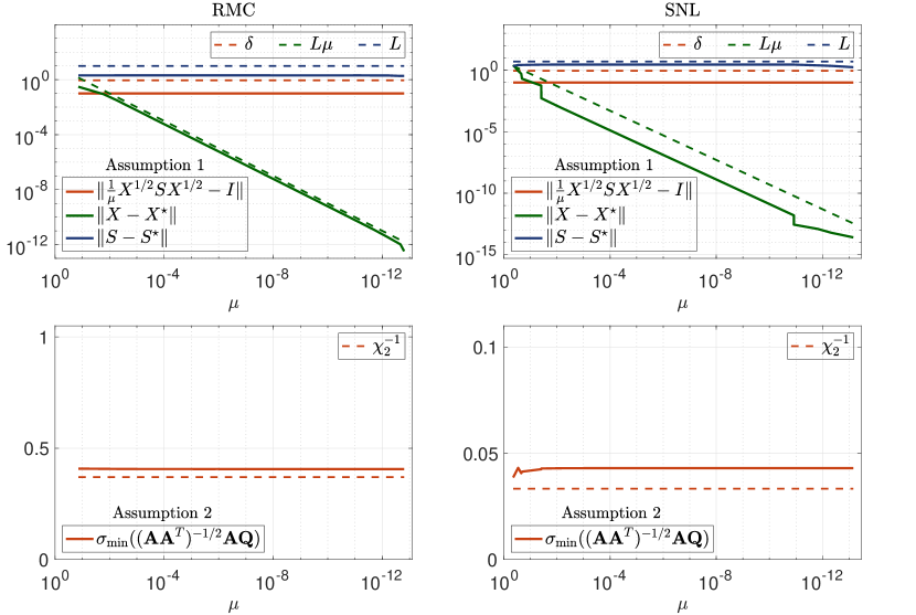
We start by verifying Assumptions 1 and 2 hold for both RMC (13) and SNL (16) problems. In Figure 2, we empirically verify both assumptions using a small-scaled RMC problem, which is generated with (n,m,mo)=(50,1200,20)(n,m,m_{o})=(50,1200,20), and a small-scaled SNL problem, which is generated with (n,m,mo)=(50,1300,25)(n,m,m_{o})=(50,1300,25). As shown in Figure 2, both assumptions hold for the RMC and SNL problems with (δ,L,χ2)=(0.9,10,2.7)(\delta,L,\chi_{2})=(0.9,10,2.7) and (δ,L,χ2)=(0.9,5,30)(\delta,L,\chi_{2})=(0.9,5,30), respectively. For these results, we run Our method and extract the primal variable XX, dual variable SS, and scaling point WW at each iteration. For each XX, SS and WW, the corresponding μ\mu is chosen such that 1μX1/2SX1/2I=0.1\|\frac{1}{\mu}X^{1/2}SX^{1/2}-I\|=0.1, and the corresponding matrix 𝐐\mathbf{Q} is constructed as in (4) with the rank parameter r=argmaxi5λi(W)/λi+1(W)r=\arg\max_{i\leq 5}\lambda_{i}(W)/\lambda_{i+1}(W).

Refer to caption
Figure 2: Verifying Assumption 1: 1μX1/2SX1/2Iδ\|\frac{1}{\mu}X^{1/2}SX^{1/2}-I\|\leq\delta, XXLμ\|X-X^{\star}\|\leq L\mu, SSL\|S-S^{\star}\|\leq L, and Assumption 2: minx(𝐀𝐀T)1/2𝐀𝐐x/𝐐xχ21\min_{x}\|(\mathbf{A}\mathbf{A}^{T})^{-1/2}\mathbf{A}\mathbf{Q}x\|/\|\mathbf{Q}x\|\geq\chi_{2}^{-1}. Left. Both assumptions hold for RMC with (δ,L,χ2)=(0.9,10,2.7)(\delta,L,\chi_{2})=(0.9,10,2.7). Right. Both assumptions hold for SNL with (δ,L,χ2)=(0.9,5,30)(\delta,L,\chi_{2})=(0.9,5,30).

Bounded condition number and PCG iterations.

As the two assumptions hold for both problems, Theorem 3.3 proves that the condition number of the corresponding indefinite system (5) is bounded and independent of μ\mu. Additionally, Corollary 3.5 shows that the indefinite system can be efficiently solved using PCG, and the number of iterations required to satisfy residual condition (Newt-ϵ\epsilon) is independent of 1/μ1/\mu.

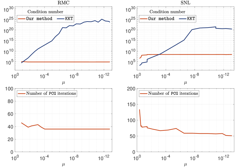
In Figure 3, we plot the condition number of our indefinite system (5) and the KKT equations (Newt-ϵ\epsilon), as well as the number of PCG iterations required to satisfy residual condition (Newt-ϵ\epsilon) with respect to different values of μ\mu. We use the same instance of RMC (13) and SNL (16) in Figure 2. For each problem, we extract WW and μ\mu as in Figure 2. For each pair of WW and μ\mu, the corresponding indefinite system is constructed as in (5) using the rank parameter r=argmaxi5λi(W)/λi+1(W)r=\arg\max_{i\leq 5}\lambda_{i}(W)/\lambda_{i+1}(W), and the corresponding KKT equations are constructed as in (Newt-ϵ\epsilon). We run PCG to solve the indefinite system until the residual condition (Newt-ϵ\epsilon) is satisfied with ϵ=106\epsilon=10^{-6}. In both cases, we see that the condition number of the indefinite system is upper bounded, while the condition number of the KKT equations (Newt-ϵ\epsilon) explodes as μ0\mu\to 0. (We note that it becomes stuck at 102510^{25} due to finite precision.) The number of PCG iterations for satisfy residual condition (Newt-ϵ\epsilon) is also bounded and independent of 1/μ1/\mu.

Refer to caption
Figure 3: Verifying Theorem 3.3: the condition number of the indefinite system (5) is bounded and independent of μ\mu, and Corollary 3.5: the number of PCG iterations required to satisfy residual condition (Newt-ϵ\epsilon) is bounded and independent of 1/μ1/\mu. Left. RMC. Right. SNL.

Cubic time complexity.

Finally, we verify Our method achieves cubic time complexity when Assumption 3 holds and rnr\ll n, with no dependence on the number of constraints mm. We first prove both RMC (13) and SNL (16) satisfy Assumption 3. Given any U,Vn×rU,V\in\mathbb{R}^{n\times r} and ymy\in\mathbb{R}^{m}. For RMC, it is obvious that both 𝒜(UVT+VUT)=Pmvec𝒮(UVT+VUT)\mathcal{A}(UV^{T}+VU^{T})=P_{m}\operatorname{vec}_{\mathcal{S}}(UV^{T}+VU^{T}) and vec𝒮(𝒜T(y))=PmTy\operatorname{vec}_{\mathcal{S}}(\mathcal{A}^{T}(y))=P_{m}^{T}y can be evaluated in O(n2r)O(n^{2}r) time and O(n2)O(n^{2}) storage. For SNL, by first paying O(kr2)O(kr^{2}) time to calculate a1a1T,,akakTa_{1}a_{1}^{T},\ldots,a_{k}a_{k}^{T}, observe that

[0eiej]T([IU][IV]T+[IV][IU]T)[0eiej],[0eiej][0eiej]T\displaystyle\begin{bmatrix}0\\ e_{i}-e_{j}\end{bmatrix}^{T}\left(\begin{bmatrix}I\\ U\end{bmatrix}\begin{bmatrix}I\\ V\end{bmatrix}^{T}+\begin{bmatrix}I\\ V\end{bmatrix}\begin{bmatrix}I\\ U\end{bmatrix}^{T}\right)\begin{bmatrix}0\\ e_{i}-e_{j}\end{bmatrix},\quad\begin{bmatrix}0\\ e_{i}-e_{j}\end{bmatrix}\begin{bmatrix}0\\ e_{i}-e_{j}\end{bmatrix}^{T}
[aiej]T([IU][IV]T+[IV][IU]T)[aiej],[aiej][aiej]T\displaystyle\begin{bmatrix}a_{i}\\ -e_{j}\end{bmatrix}^{T}\left(\begin{bmatrix}I\\ U\end{bmatrix}\begin{bmatrix}I\\ V\end{bmatrix}^{T}+\begin{bmatrix}I\\ V\end{bmatrix}\begin{bmatrix}I\\ U\end{bmatrix}^{T}\right)\begin{bmatrix}a_{i}\\ -e_{j}\end{bmatrix},\quad\begin{bmatrix}a_{i}\\ -e_{j}\end{bmatrix}\begin{bmatrix}a_{i}\\ -e_{j}\end{bmatrix}^{T}

can all be evaluated in O(r)O(r) time. (Notice that r=dr=d in SNR.) Therefore, when knk\ll n, which is common in real-world applications where there are typically more sensors than anchors, both 𝒜(X)\mathcal{A}(X) and 𝒜T(y)U\mathcal{A}^{T}(y)U can be evaluated in O(n2r)O(n^{2}r) time and O(n2)O(n^{2}) storage.

Refer to caption
Figure 4: Verifying cubic time complexity for Our method: both setting up the indefinite system (5) and one iteration of PCG cost O(n3)O(n^{3}) time, with no dependency on the number of constraints mm. Left. RMC with m=O(n)m=O(n) and m=O(n2)m=O(n^{2}). Right. SNL with m=O(n)m=O(n) and m=O(n2)m=O(n^{2}).

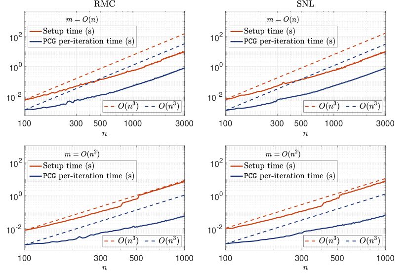
In Figure 4, we plot the average setup time for the indefinite system (5) and the average per PCG iteration time against nn for both RMC and SNL problem. Specifically, the setup time includes: the time to decompose W=QΛQT+QΛQTW=Q\Lambda Q^{T}+Q_{\perp}\Lambda_{\perp}Q_{\perp}^{T} and construct E=QQT+τ1QΛQTE=QQ^{T}+\tau^{-1}Q_{\perp}\Lambda_{\perp}Q_{\perp}^{T} in order to implicitly setup 𝐐\mathbf{Q}, 𝐄\mathbf{E}, and 𝚺\mathbf{\Sigma} as in (4); explicitly form the Schur complement 𝐂=τ2𝚺+β1𝐐T𝐀T𝐀𝐐\mathbf{C}=\tau^{2}\mathbf{\Sigma}+\beta^{-1}\mathbf{Q}^{T}\mathbf{A}^{T}\mathbf{A}\mathbf{Q} via O(nr)O(nr) matrix-vector product with 𝐀𝐐\mathbf{A}\mathbf{Q} and 𝐐T𝐀T\mathbf{Q}^{T}\mathbf{A}^{T}; and compute the Cholesky factor of 𝐂\mathbf{C}. We consider two cases, m=O(n)m=O(n) and m=O(n2)m=O(n^{2}), in order to verify the time complexity of Our method is indeed invariant to mm. For both problem, we set the number of constraints to be m=20nm=20n for the case of m=O(n)m=O(n), and m=n(n1)/2m=n(n-1)/2 for the case of m=O(n2)m=O(n^{2}). As we are interested in measuring the run time of Our method for solving the standard form SDP (1a), we fix mo=0m_{o}=0 to eliminate all the LP constraint in (13) and (16). As shown in Figure 4, the setup time and per PCG time exhibit cubic time complexity for both problems.

7.2 Comparison against other approaches

Table 1: Reconstruction error (Error) and runtime (Time) for solving rank-22 size n×nn\times n RMC problems with mm constraints and mom_{o} outliers.
nn mm mom_{o} Our method MOSEK ZL17 ADMM
Error Time Error Time Error Time Error Time
100 3000 12 1.2𝐞𝟏𝟐\boldsymbol{1.2\mathrm{e}\raisebox{0.3pt}{\scalebox{0.7}{$-$}}12} 1.2s 2.3e102.3\mathrm{e}\raisebox{0.3pt}{\scalebox{0.7}{$-$}}10 2.5s 2.7e062.7\mathrm{e}\raisebox{0.3pt}{\scalebox{0.7}{$-$}}06 1.6s 7.4e077.4\mathrm{e}\raisebox{0.3pt}{\scalebox{0.7}{$-$}}07 24.6s
100 4000 24 1.5𝐞𝟏𝟐\boldsymbol{1.5\mathrm{e}\raisebox{0.3pt}{\scalebox{0.7}{$-$}}12} 1.0s 2.3e112.3\mathrm{e}\raisebox{0.3pt}{\scalebox{0.7}{$-$}}11 5.3s 2.2e062.2\mathrm{e}\raisebox{0.3pt}{\scalebox{0.7}{$-$}}06 1.7s 8.4e078.4\mathrm{e}\raisebox{0.3pt}{\scalebox{0.7}{$-$}}07 25.9s
100 5000 48 1.9𝐞𝟏𝟐\boldsymbol{1.9\mathrm{e}\raisebox{0.3pt}{\scalebox{0.7}{$-$}}12} 2.2s 1.5e081.5\mathrm{e}\raisebox{0.3pt}{\scalebox{0.7}{$-$}}08 6.8s 9.6e069.6\mathrm{e}\raisebox{0.3pt}{\scalebox{0.7}{$-$}}06 2.2s 7.5e077.5\mathrm{e}\raisebox{0.3pt}{\scalebox{0.7}{$-$}}07 152s
300 40000 50 3.1𝐞𝟏𝟐\boldsymbol{3.1\mathrm{e}\raisebox{0.3pt}{\scalebox{0.7}{$-$}}12} 21.7s 2.6e092.6\mathrm{e}\raisebox{0.3pt}{\scalebox{0.7}{$-$}}09 1853s 1.6e061.6\mathrm{e}\raisebox{0.3pt}{\scalebox{0.7}{$-$}}06 31.3s 7.0e077.0\mathrm{e}\raisebox{0.3pt}{\scalebox{0.7}{$-$}}07 84.2s
300 42500 100 4.2𝐞𝟏𝟐\boldsymbol{4.2\mathrm{e}\raisebox{0.3pt}{\scalebox{0.7}{$-$}}12} 23.9s 2.7e072.7\mathrm{e}\raisebox{0.3pt}{\scalebox{0.7}{$-$}}07 2218s 3.9e063.9\mathrm{e}\raisebox{0.3pt}{\scalebox{0.7}{$-$}}06 42.0s 8.9e078.9\mathrm{e}\raisebox{0.3pt}{\scalebox{0.7}{$-$}}07 48.5s
300 45000 150 5.0𝐞𝟏𝟐\boldsymbol{5.0\mathrm{e}\raisebox{0.3pt}{\scalebox{0.7}{$-$}}12} 32.1s 3.6e113.6\mathrm{e}\raisebox{0.3pt}{\scalebox{0.7}{$-$}}11 2310s 7.4e077.4\mathrm{e}\raisebox{0.3pt}{\scalebox{0.7}{$-$}}07 67.9s 8.5e078.5\mathrm{e}\raisebox{0.3pt}{\scalebox{0.7}{$-$}}07 50.1s
500 115000 100 7.0𝐞𝟏𝟐\boldsymbol{7.0\mathrm{e}\raisebox{0.3pt}{\scalebox{0.7}{$-$}}12} 127s Out of memory 7.5e067.5\mathrm{e}\raisebox{0.3pt}{\scalebox{0.7}{$-$}}06 154s 6.7e076.7\mathrm{e}\raisebox{0.3pt}{\scalebox{0.7}{$-$}}07 103s
500 120000 200 7.9𝐞𝟏𝟐\boldsymbol{7.9\mathrm{e}\raisebox{0.3pt}{\scalebox{0.7}{$-$}}12} 138s Out of memory 1.7e061.7\mathrm{e}\raisebox{0.3pt}{\scalebox{0.7}{$-$}}06 260s 7.6e077.6\mathrm{e}\raisebox{0.3pt}{\scalebox{0.7}{$-$}}07 180s
500 125000 300 7.4𝐞𝟏𝟐\boldsymbol{7.4\mathrm{e}\raisebox{0.3pt}{\scalebox{0.7}{$-$}}12} 127s Out of memory 6.2e066.2\mathrm{e}\raisebox{0.3pt}{\scalebox{0.7}{$-$}}06 233s 8.0e078.0\mathrm{e}\raisebox{0.3pt}{\scalebox{0.7}{$-$}}07 314s
1000 400000 150 1.3𝐞𝟏𝟏\boldsymbol{1.3\mathrm{e}\raisebox{0.3pt}{\scalebox{0.7}{$-$}}11} 1011s Out of memory 1.5e061.5\mathrm{e}\raisebox{0.3pt}{\scalebox{0.7}{$-$}}06 2253s 7.5e077.5\mathrm{e}\raisebox{0.3pt}{\scalebox{0.7}{$-$}}07 522s
1000 450000 300 1.1𝐞𝟏𝟏\boldsymbol{1.1\mathrm{e}\raisebox{0.3pt}{\scalebox{0.7}{$-$}}11} 954s Out of memory 9.7e079.7\mathrm{e}\raisebox{0.3pt}{\scalebox{0.7}{$-$}}07 1675s 2.2e072.2\mathrm{e}\raisebox{0.3pt}{\scalebox{0.7}{$-$}}07 594s
1000 500000 450 1.2𝐞𝟏𝟏\boldsymbol{1.2\mathrm{e}\raisebox{0.3pt}{\scalebox{0.7}{$-$}}11} 1106s Out of memory 2.1e052.1\mathrm{e}\raisebox{0.3pt}{\scalebox{0.7}{$-$}}05 1458s 9.4e079.4\mathrm{e}\raisebox{0.3pt}{\scalebox{0.7}{$-$}}07 1027s

In this section, we compare the practical performance of Our method for solving both robust matrix completion and sensor network localization problems.

Robust matrix completion.

First-order methods, such as linearized alternating direction method of multipliers (ADMM) [50, 19], can be used to solve (12) via the following iterations:

Xk+1=𝒫r(Xkαfλ(Xk,sk,yk)),sk+1=𝒮λ/β(𝒜(Xk+1)+ykb),yk+1=yk+β(𝒜(Xk+1)sk+1b)\displaystyle\begin{split}X_{k+1}&=\mathcal{P}_{r}(X_{k}-\alpha\nabla f_{\lambda}(X_{k},s_{k},y_{k})),\\ s_{k+1}&=\mathcal{S}_{\lambda/\beta}(\mathcal{A}(X_{k+1})+y_{k}-b),\\ y_{k+1}&=y_{k}+\beta(\mathcal{A}(X_{k+1})-s_{k+1}-b)\end{split} (17)

where α=n2m\alpha=\frac{n^{2}}{m}, β\beta is the step size, fλ(X,s,y)=β2𝒜(X)bs+y2+λtr(X)f_{\lambda}(X,s,y)=\frac{\beta}{2}\|\mathcal{A}(X)-b-s+y\|^{2}+\lambda\operatorname{tr}(X), 𝒫r(X)\mathcal{P}_{r}(X) denotes the projection of XX onto a set of rank-rr matrices, and 𝒮γ(x)=max{xγ,0}+min{x+γ,0}\mathcal{S}_{\gamma}(x)=\max\{x-\gamma,0\}+\min\{x+\gamma,0\} is the soft-thresholding operator. While fast, the convergence of ADMM is not guaranteed without additional assumption on XX^{\star}, such as requiring XX^{\star} to be incoherent in the context of matrix completion. This makes it less reliable for obtaining high accuracy solutions.

Alternatively, the Burer–Monteiro (BM) approach can be applied by substituting X=UUTX=UU^{T} where Un×rU\in\mathbb{R}^{n\times r} and rrank(X)r\geq\mathrm{rank}\,(X^{\star}). Unfortunately, as we explained in the introduction, the Burer–Monteiro approach is not able to solve the problem satisfactorily as it would either solve the problem by substituting X=UUTX=UU^{T} into (12) or (13). The former is an unconstrained nonsmooth problem, which can be solved via subgradient (SubGD) method Uk+1=Ukαf(Uk)U_{k+1}=U_{k}-\alpha\nabla f(U_{k}) with step-size α(0,1]\alpha\in(0,1] and f(U)=𝒜(UUT)b1+λUF2f(U)=\|\mathcal{A}(UU^{T})-b\|_{1}+\lambda\|U\|_{F}^{2}. The latter is a constrained twice-differentiable problem, which can be solved via nonlinear programming (NLP) solver like Fmincon [33] and Knitro [13]. But in both cases, local optimization algorithms can struggle to converge, because the underlying nonsmoothness of the problem is further exacerbated by the nonconvexity of the BM factorization.

A promising alternative is to solve (13) via general-purpose IPM solver such as MOSEK [34]. However, general-purpose IPM incurs at least Ω((n+m)3)\Omega((n+m)^{3}) time and Ω((n+m)2)\Omega((n+m)^{2}) memory, which is concerning for problem instances with m=O(n2)m=O(n^{2}) measurements.

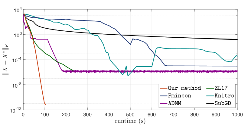
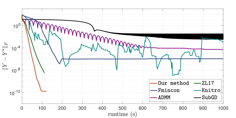
Instead, we present experimental evidence to show that Our method is the most reliable way of solving RMC to high accuracies. We start by demonstrating the efficiency and efficacy of Our method by solving a large-scaled RMC, which is generated with (n,m,mo)=(500,125250,250)(n,m,m_{o})=(500,125250,250). In Figure 1, we plot the reconstruction error XXF\|X-X^{\star}\|_{F} against runtime for Our method, ZL17, Fmincon, Knitro, ADMM and SubGD. Here, the maximum rank parameter r^\hat{r} for Our method, and the search rank rr for Fmincon, Knitro, ADMM and SubGD are all set to be r=10r=10. We initialized Fmincon, Knitro and SubGD at the same initial point U0U_{0} that is drawn from standard Gaussian, and initialized ADMM at X0=U0U0TX_{0}=U_{0}U_{0}^{T}. The step-size of ADMM and SubGD is set be β=102\beta=10^{-2} and α=106\alpha=10^{-6}, respectively. From Figure 1, we see that Our method is the only one that is able to achieve reconstruction error below 10810^{-8}. Though both ADMM and ZL17 achieves reconstruction error 10610^{-6} at the fastest rate, they cannot make any further progress; ADMM becomes stuck and ZL17 becomes ill-conditioned. Comparing to nonlinear programming solvers, both Fmincon and Knitro eventually reach the same reconstruction error similar to ZL17 but at a significantly slower rate than Our method. Finally, SubGD converges extremely slowly for this problem.

Refer to caption
Figure 5: Reconstruction error YYF\|Y-Y^{\star}\|_{F} against runtime for solving an instance of SNL problem (16) using Our method, ZL17, Fmincon, Knitro, ADMM, and SubGD. The SNL problem is generated with (n,m,m0)=(300,45000,300)(n,m,m_{0})=(300,45000,300).

In Table 1, we solve several instances of RMC problems using Our method, MOSEK, ZL17 and ADMM, and report their corresponding reconstruction error and runtime. For space efficiency, we omit the comparison with Knitro, Fmincon and SubGD as they generally perform worse than ADMM. In this experiment, the maximum rank parameter r^\hat{r} for Our method and the search rank r^\hat{r} for ADMM are all set to be 1010. The number of iterations for ADMM is set to be 10510^{5}. For all four methods, we report the best reconstruction error and the time they achieve their best reconstruction error. From Table 1, we see that Our method consistently achieves reconstruction error around 101210^{-12} in all cases, with runtime similar to ZL17. For n=500n=500 and larger, MOSEK runs out of memory. We note that we pick the largest possible step size for ADMM that allows it to stably converge to the smallest error.

Sensor network localization.

We again demonstrate the efficiency and efficacy of Our method by solving a large-scale SNL problem, which is generated with (n,m,mo)=(300,45000,300)(n,m,m_{o})=(300,45000,300). Similar to RMC, SNL can also be solved via Fmincon, Knitro, ADMM and SubGD. In particular, ADMM can be applied by first rewriting (16) into the standard form minX0𝒜(X)b1\min_{X\succeq 0}\|\mathcal{A}(X)-b\|_{1}, and then apply (17) with λ=0\lambda=0. The SubGD method can subsequently be applied with the update Uk+1=Ukαf(Uk)U_{k+1}=U_{k}-\alpha\nabla f(U_{k}), where α(0,1]\alpha\in(0,1], Un×rU\in\mathbb{R}^{n\times r}, and f(U)=𝒜(UUT)b1f(U)=\|\mathcal{A}(UU^{T})-b\|_{1}. Finally, both Fmincon and Knitro can be applied by substituting X=UUTX=UU^{T} into (16).

In Figure 5, we plot the reconstruction error against runtime for Our method, ZL17, Fmincon, Knitro, ADMM and SubGD. The reconstruction error for SNL is defined as YYF\|Y-Y^{\star}\|_{F} where Y=[y1,,yn]Y^{\star}=[y_{1}^{\star},\ldots,y_{n}^{\star}]. Here, the maximum rank parameter r^\hat{r} for Our method, and the search rank rr for Fmincon, Knitro, ADMM and SubGD are all set to be r=10r=10. We initialized Fmincon, Knitro and SubGD at the same initial point U0U_{0} that is drawn from standard Gaussian, and initialized ADMM at X0=U0U0TX_{0}=U_{0}U_{0}^{T}. The step-size of ADMM and SubGD is set be β=0.03\beta=0.03 and α=5×10⁶\alpha=5\times 10^{-6}, respectively. From Figure 5, we again see that Our method is the only one that is able to achieve reconstruction error around 101210^{-12} at the fastest rate.

In Table 2, we solve several instances of SNL problems using Our method, MOSEK, ZL17 and Knitro, and report their corresponding reconstruction error and runtime. For simplicity, we omit the comparison with ADMM, Fmincon, and SubGD as they generally perform worse than Knitro. In this experiment, the maximum rank parameter r^\hat{r} for Our method and the search rank r^\hat{r} for Knitro are all set to be 1010. The number of iterations for Knitro is set to be 500500. For all four method, we report the best reconstruction error and the time they achieve their best reconstruction error. As shown in Table 2, Our method again consistently achieves reconstruction error around 101210^{-12} in all cases, with runtime similar to ZL17. For n=500n=500 and larger, MOSEK runs out of memory.

Table 2: Reconstruction error (Error) and runtime (Time) for solving 2-dimensional SNL problems with nn sensors, 3 anchors, mm distance measurements and mom_{o} outliers.
nn mm mom_{o} Our method MOSEK ZL17 Knitro
Error Time Error Time Error Time Error Time
50 1000 30 2.9𝐞𝟏𝟑\boldsymbol{2.9\mathrm{e}\raisebox{0.3pt}{\scalebox{0.7}{$-$}}13} 1.0s 1.1e091.1\mathrm{e}\raisebox{0.3pt}{\scalebox{0.7}{$-$}}09 0.6s 5.6e105.6\mathrm{e}\raisebox{0.3pt}{\scalebox{0.7}{$-$}}10 1.1s 4.5e104.5\mathrm{e}\raisebox{0.3pt}{\scalebox{0.7}{$-$}}10 7.0s
50 1150 40 2.4𝐞𝟏𝟑\boldsymbol{2.4\mathrm{e}\raisebox{0.3pt}{\scalebox{0.7}{$-$}}13} 0.7s 9.3e139.3\mathrm{e}\raisebox{0.3pt}{\scalebox{0.7}{$-$}}13 0.5s 1.2e091.2\mathrm{e}\raisebox{0.3pt}{\scalebox{0.7}{$-$}}09 0.8s 4.3e104.3\mathrm{e}\raisebox{0.3pt}{\scalebox{0.7}{$-$}}10 9.2s
50 1300 50 1.7𝐞𝟏𝟑\boldsymbol{1.7\mathrm{e}\raisebox{0.3pt}{\scalebox{0.7}{$-$}}13} 0.6s 4.5e124.5\mathrm{e}\raisebox{0.3pt}{\scalebox{0.7}{$-$}}12 0.7s 8.8e108.8\mathrm{e}\raisebox{0.3pt}{\scalebox{0.7}{$-$}}10 0.8s 4.6e104.6\mathrm{e}\raisebox{0.3pt}{\scalebox{0.7}{$-$}}10 14.6s
100 3000 60 4.3𝐞𝟏𝟑\boldsymbol{4.3\mathrm{e}\raisebox{0.3pt}{\scalebox{0.7}{$-$}}13} 2.2s 1.2e121.2\mathrm{e}\raisebox{0.3pt}{\scalebox{0.7}{$-$}}12 3.2s 3.0e093.0\mathrm{e}\raisebox{0.3pt}{\scalebox{0.7}{$-$}}09 3.1s 8.4e098.4\mathrm{e}\raisebox{0.3pt}{\scalebox{0.7}{$-$}}09 64.4s
100 4000 80 8.5𝐞𝟏𝟑\boldsymbol{8.5\mathrm{e}\raisebox{0.3pt}{\scalebox{0.7}{$-$}}13} 2.9s 1.1e101.1\mathrm{e}\raisebox{0.3pt}{\scalebox{0.7}{$-$}}10 4.4s 3.8e093.8\mathrm{e}\raisebox{0.3pt}{\scalebox{0.7}{$-$}}09 3.4s 3.9e113.9\mathrm{e}\raisebox{0.3pt}{\scalebox{0.7}{$-$}}11 53.7s
100 5000 100 4.2𝐞𝟏𝟑\boldsymbol{4.2\mathrm{e}\raisebox{0.3pt}{\scalebox{0.7}{$-$}}13} 4.1s 1.3e101.3\mathrm{e}\raisebox{0.3pt}{\scalebox{0.7}{$-$}}10 7.8s 1.0e081.0\mathrm{e}\raisebox{0.3pt}{\scalebox{0.7}{$-$}}08 3.8s 2.1e082.1\mathrm{e}\raisebox{0.3pt}{\scalebox{0.7}{$-$}}08 59.2s
300 40000 220 2.2𝐞𝟏𝟐\boldsymbol{2.2\mathrm{e}\raisebox{0.3pt}{\scalebox{0.7}{$-$}}12} 108.5s 5.6e105.6\mathrm{e}\raisebox{0.3pt}{\scalebox{0.7}{$-$}}10 1801s 1.8e091.8\mathrm{e}\raisebox{0.3pt}{\scalebox{0.7}{$-$}}09 136.2s 1.5e091.5\mathrm{e}\raisebox{0.3pt}{\scalebox{0.7}{$-$}}09 415.4s
300 42500 260 1.7𝐞𝟏𝟐\boldsymbol{1.7\mathrm{e}\raisebox{0.3pt}{\scalebox{0.7}{$-$}}12} 95.3s 3.7e113.7\mathrm{e}\raisebox{0.3pt}{\scalebox{0.7}{$-$}}11 2439s 1.5e091.5\mathrm{e}\raisebox{0.3pt}{\scalebox{0.7}{$-$}}09 119.3s 2.7e092.7\mathrm{e}\raisebox{0.3pt}{\scalebox{0.7}{$-$}}09 275.9s
300 45000 300 1.6𝐞𝟏𝟐\boldsymbol{1.6\mathrm{e}\raisebox{0.3pt}{\scalebox{0.7}{$-$}}12} 117.5s 2.5e112.5\mathrm{e}\raisebox{0.3pt}{\scalebox{0.7}{$-$}}11 3697s 3.3e093.3\mathrm{e}\raisebox{0.3pt}{\scalebox{0.7}{$-$}}09 111.7s 1.2e091.2\mathrm{e}\raisebox{0.3pt}{\scalebox{0.7}{$-$}}09 749.0s
500 100000 420 5.9𝐞𝟏𝟐\boldsymbol{5.9\mathrm{e}\raisebox{0.3pt}{\scalebox{0.7}{$-$}}12} 499.3s Out of memory 1.5e091.5\mathrm{e}\raisebox{0.3pt}{\scalebox{0.7}{$-$}}09 592.8s 9.9e109.9\mathrm{e}\raisebox{0.3pt}{\scalebox{0.7}{$-$}}10 2548s
550 110000 460 2.6𝐞𝟏𝟐\boldsymbol{2.6\mathrm{e}\raisebox{0.3pt}{\scalebox{0.7}{$-$}}12} 559.4s Out of memory 6.8e096.8\mathrm{e}\raisebox{0.3pt}{\scalebox{0.7}{$-$}}09 747.7s 4.1e094.1\mathrm{e}\raisebox{0.3pt}{\scalebox{0.7}{$-$}}09 1081s
500 120000 500 6.0𝐞𝟏𝟐\boldsymbol{6.0\mathrm{e}\raisebox{0.3pt}{\scalebox{0.7}{$-$}}12} 760.5s Out of memory 2.1e082.1\mathrm{e}\raisebox{0.3pt}{\scalebox{0.7}{$-$}}08 955.5s 1.2e091.2\mathrm{e}\raisebox{0.3pt}{\scalebox{0.7}{$-$}}09 595.0s

References

  • [1] A. Y. Alfakih, A. Khandani, and H. Wolkowicz, Solving euclidean distance matrix completion problems via semidefinite programming, Computational optimization and applications, 12 (1999), pp. 13–30.
  • [2] F. Alizadeh, J.-P. A. Haeberly, and M. L. Overton, Complementarity and nondegeneracy in semidefinite programming, Mathematical Programming, 77 (1997), pp. 111–128.
  • [3] T. Ando, Concavity of certain maps on positive definite matrices and applications to hadamard products, Linear Algebra and its Applications, 26 (1979), pp. 203–241.
  • [4] S. Bellavia, J. Gondzio, and B. Morini, A matrix-free preconditioner for sparse symmetric positive definite systems and least-squares problems, SIAM Journal on Scientific Computing, 35 (2013), pp. A192–A211.
  • [5] S. Bellavia, J. Gondzio, and M. Porcelli, An inexact dual logarithmic barrier method for solving sparse semidefinite programs, Mathematical Programming, 178 (2019), pp. 109–143.
  • [6] S. J. Benson, Y. Ye, and X. Zhang, Solving large-scale sparse semidefinite programs for combinatorial optimization, SIAM Journal on Optimization, 10 (2000), pp. 443–461.
  • [7] L. Bergamaschi, J. Gondzio, and G. Zilli, Preconditioning indefinite systems in interior point methods for optimization, Computational Optimization and Applications, 28 (2004), pp. 149–171.
  • [8] P. Biswas and Y. Ye, Semidefinite programming for ad hoc wireless sensor network localization, in Proceedings of the 3rd international symposium on Information processing in sensor networks, 2004, pp. 46–54.
  • [9] E. Y. Bobrovnikova and S. A. Vavasis, Accurate solution of weighted least squares by iterative methods, SIAM Journal on Matrix Analysis and Applications, 22 (2001), pp. 1153–1174.
  • [10] N. Boumal, Nonconvex phase synchronization, SIAM Journal on Optimization, 26 (2016), pp. 2355–2377.
  • [11] N. Boumal, V. Voroninski, and A. S. Bandeira, Deterministic guarantees for burer-monteiro factorizations of smooth semidefinite programs, Communications on Pure and Applied Mathematics, 73 (2020), pp. 581–608.
  • [12] S. Burer and R. D. Monteiro, A nonlinear programming algorithm for solving semidefinite programs via low-rank factorization, Math. Program., 95 (2003), pp. 329–357.
  • [13] R. H. Byrd, J. Nocedal, and R. A. Waltz, K nitro: An integrated package for nonlinear optimization, Large-scale nonlinear optimization, (2006), pp. 35–59.
  • [14] J.-F. Cai, E. J. Candès, and Z. Shen, A singular value thresholding algorithm for matrix completion, SIAM Journal on Optimization, 20 (2010), pp. 1956–1982.
  • [15] E. Candès and B. Recht, Exact matrix completion via convex optimization., Foundations of Computational Mathematics, 9 (2009).
  • [16] E. J. Candès, X. Li, Y. Ma, and J. Wright, Robust principal component analysis?, Journal of the ACM (JACM), 58 (2011), pp. 1–37.
  • [17] E. J. Candes and Y. Plan, Tight oracle inequalities for low-rank matrix recovery from a minimal number of noisy random measurements, IEEE Transactions on Information Theory, 57 (2011), pp. 2342–2359.
  • [18] E. J. Candes, T. Strohmer, and V. Voroninski, Phaselift: Exact and stable signal recovery from magnitude measurements via convex programming, Communications on Pure and Applied Mathematics, 66 (2013), pp. 1241–1274.
  • [19] Y. Cherapanamjeri, K. Gupta, and P. Jain, Nearly optimal robust matrix completion, in International Conference on Machine Learning, PMLR, 2017, pp. 797–805.
  • [20] H.-M. Chiu and R. Y. Zhang, Tight certification of adversarially trained neural networks via nonconvex low-rank semidefinite relaxations, in International Conference on Machine Learning, PMLR, 2023, pp. 5631–5660.
  • [21] L. Ding, L. Jiang, Y. Chen, Q. Qu, and Z. Zhu, Rank overspecified robust matrix recovery: Subgradient method and exact recovery, Advances in Neural Information Processing Systems, 34 (2021), pp. 26767–26778.
  • [22] V. Faber and T. Manteuffel, Necessary and sufficient conditions for the existence of a conjugate gradient method, SIAM Journal on numerical analysis, 21 (1984), pp. 352–362.
  • [23] M. Fukuda, M. Kojima, K. Murota, and K. Nakata, Exploiting sparsity in semidefinite programming via matrix completion I: General framework, SIAM J. Optim., 11 (2001), pp. 647–674.
  • [24] J. Gondzio, Matrix-free interior point method, Computational Optimization and Applications, 51 (2012), pp. 457–480.
  • [25] N. I. Gould, Iterative methods for ill-conditioned linear systems from optimization, Springer, 2000.
  • [26] A. Greenbaum, Iterative methods for solving linear systems, SIAM, 1997.
  • [27] S. Habibi, M. Kočvara, and M. Stingl, Loraine–an interior-point solver for low-rank semidefinite programming, Optimization Methods and Software, (2023), pp. 1–31.
  • [28] S. Kim, M. Kojima, M. Mevissen, and M. Yamashita, Exploiting sparsity in linear and nonlinear matrix inequalities via positive semidefinite matrix completion, Math. Program., 129 (2011), pp. 33–68.
  • [29] L. Lukšan and J. Vlček, Indefinitely preconditioned inexact newton method for large sparse equality constrained non-linear programming problems, Numerical linear algebra with applications, 5 (1998), pp. 219–247.
  • [30] Z.-Q. Luo, J. F. Sturm, and S. Zhang, Superlinear convergence of a symmetric primal-dual path following algorithm for semidefinite programming, SIAM Journal on Optimization, 8 (1998), pp. 59–81.
  • [31] J. Ma and S. Fattahi, Global convergence of sub-gradient method for robust matrix recovery: Small initialization, noisy measurements, and over-parameterization, Journal of Machine Learning Research, 24 (2023), pp. 1–84.
  • [32] S. Maniu, P. Senellart, and S. Jog, An experimental study of the treewidth of real-world graph data, in 22nd International Conference on Database Theory (ICDT 2019), Schloss Dagstuhl-Leibniz-Zentrum fuer Informatik, 2019.
  • [33] Matlab optimization toolbox, 2021. The MathWorks, Natick, MA, USA.
  • [34] MOSEK ApS, The MOSEK optimization toolbox for MATLAB manual. Version 7.1 (Revision 28)., 2015.
  • [35] Y. E. Nesterov and M. J. Todd, Self-scaled barriers and interior-point methods for convex programming, Mathematics of Operations research, 22 (1997), pp. 1–42.
  • [36]  , Primal-dual interior-point methods for self-scaled cones, SIAM Journal on optimization, 8 (1998), pp. 324–364.
  • [37] B. Recht, M. Fazel, and P. A. Parrilo, Guaranteed minimum-rank solutions of linear matrix equations via nuclear norm minimization, SIAM review, 52 (2010), pp. 471–501.
  • [38] D. M. Rosen, L. Carlone, A. S. Bandeira, and J. J. Leonard, Se-sync: A certifiably correct algorithm for synchronization over the special euclidean group, The International Journal of Robotics Research, 38 (2019), pp. 95–125.
  • [39] M. Rozlozník and V. Simoncini, Krylov subspace methods for saddle point problems with indefinite preconditioning, SIAM journal on matrix analysis and applications, 24 (2002), pp. 368–391.
  • [40] A. M.-C. So and Y. Ye, Theory of semidefinite programming for sensor network localization, Mathematical Programming, 109 (2007), pp. 367–384.
  • [41] J. F. Sturm, Using SeDuMi 1.02, a MATLAB toolbox for optimization over symmetric cones, Optimization methods and software, 11 (1999), pp. 625–653.
  • [42]  , Implementation of interior point methods for mixed semidefinite and second order cone optimization problems, Optim. Method. Softw., 17 (2002), pp. 1105–1154.
  • [43] J. F. Sturm and S. Zhang, Symmetric primal-dual path-following algorithms for semidefinite programming, Applied Numerical Mathematics, 29 (1999), pp. 301–315.
  • [44] K.-C. Toh, Solving large scale semidefinite programs via an iterative solver on the augmented systems, SIAM Journal on Optimization, 14 (2004), pp. 670–698.
  • [45] K.-C. Toh and M. Kojima, Solving some large scale semidefinite programs via the conjugate residual method, SIAM Journal on Optimization, 12 (2002), pp. 669–691.
  • [46] K.-C. Toh, M. J. Todd, and R. H. Tütüncü, Sdpt3–a matlab software package for semidefinite programming, version 1.3, Optimization methods and software, 11 (1999), pp. 545–581.
  • [47] L. Vandenberghe and S. Boyd, Semidefinite programming, SIAM review, 38 (1996), pp. 49–95.
  • [48] S. J. Wright, Primal-dual interior-point methods, SIAM, 1997.
  • [49] H. Yang, L. Liang, L. Carlone, and K.-C. Toh, An inexact projected gradient method with rounding and lifting by nonlinear programming for solving rank-one semidefinite relaxation of polynomial optimization, Mathematical Programming, 201 (2023), pp. 409–472.
  • [50] X. Yuan and J. Yang, Sparse and low-rank matrix decomposition via alternating direction methods, preprint, 12 (2009).
  • [51] A. Yurtsever, J. A. Tropp, O. Fercoq, M. Udell, and V. Cevher, Scalable semidefinite programming, SIAM Journal on Mathematics of Data Science, 3 (2021), pp. 171–200.
  • [52] R. Y. Zhang, Parameterized complexity of chordal conversion for sparse semidefinite programs with small treewidth, arXiv preprint arXiv:2306.15288, (2023).
  • [53] R. Y. Zhang and J. Lavaei, Modified interior-point method for large-and-sparse low-rank semidefinite programs, in IEEE 56th Conference on Decision and Control, 2017.
  • [54]  , Sparse semidefinite programs with guaranteed near-linear time complexity via dualized clique tree conversion, Mathematical programming, 188 (2021), pp. 351–393.

Appendix A Proof of Proposition 3.2

We break the proof into three parts. Below, recall that we have defined Ψn\Psi_{n} as the basis matrix for vec(𝒮n)\operatorname{vec}(\mathcal{S}^{n}) on vec(n×n)=n2\operatorname{vec}(\mathbb{R}^{n\times n})=\mathbb{R}^{n^{2}}, in order to define vec𝒮(X)=defΨnTvec(X)=12ΨnTvec(X+XT)\operatorname{vec}_{\mathcal{S}}(X)\overset{\mathrm{def}}{=}\Psi_{n}^{T}\operatorname{vec}(X)=\frac{1}{2}\Psi_{n}^{T}\operatorname{vec}(X+X^{T}) for Xn×nX\in\mathbb{R}^{n\times n}, and A𝒮B=B𝒮A=def12ΨnT(AB+BA)ΨrA\otimes_{\mathcal{S}}B=B\otimes_{\mathcal{S}}A\overset{\mathrm{def}}{=}\frac{1}{2}\Psi_{n}^{T}(A\otimes B+B\otimes A)\Psi_{r} for A,Bn×rA,B\in\mathbb{R}^{n\times r}.

Lemma A.1 (Correctness).

Let W=QΛQT+QΛQTW=Q\Lambda Q^{T}+Q_{\perp}\Lambda_{\perp}Q_{\perp}^{T} where [Q,Q][Q,Q_{\perp}] is orthonormal, and pick 0<τ<λmin(Λ)0<\tau<\lambda_{\min}(\Lambda). Define E=QQT+τ1QΛQT,E=QQ^{T}+\tau^{-1}\cdot Q_{\perp}\Lambda_{\perp}Q_{\perp}^{T}, 𝐐B=Q𝒮Q,\mathbf{Q}_{B}=Q\otimes_{\mathcal{S}}Q, 𝐐N=2ΨnT(QQ),\mathbf{Q}_{N}=\sqrt{2}\Psi_{n}^{T}(Q\otimes Q_{\perp}), 𝚺B1=Λ𝒮Λτ2I,\mathbf{\Sigma}_{B}^{-1}=\Lambda\otimes_{\mathcal{S}}\Lambda-\tau^{2}I, and 𝚺N1=(ΛτI)Λ\mathbf{\Sigma}_{N}^{-1}=(\Lambda-\tau I)\otimes\Lambda_{\perp}. Then

W𝒮W=[𝐐B,𝐐N][𝚺B𝚺N]1[𝐐B,𝐐N]T+τ2E𝒮E.W\otimes_{\mathcal{S}}W=[\mathbf{Q}_{B},\mathbf{Q}_{N}]\begin{bmatrix}\mathbf{\Sigma}_{B}\\ &\mathbf{\Sigma}_{N}\end{bmatrix}^{-1}[\mathbf{Q}_{B},\mathbf{Q}_{N}]^{T}+\tau^{2}\cdot E\otimes_{\mathcal{S}}E.
Proof.

Write WX=τQ(ΛτI)QTW_{X}=\tau\cdot Q(\Lambda-\tau I)Q^{T} and WS=τ1QΛQTW_{S}=\tau^{-1}Q_{\perp}\Lambda_{\perp}Q_{\perp}^{T}. For arbitrary Y𝒮nY\in\mathcal{S}^{n}, it follows from W=τE+τ1WXW=\tau E+\tau^{-1}W_{X} that

ΨnT(WW)Ψnvec𝒮(Y)=\displaystyle\Psi_{n}^{T}(W\otimes W)\Psi_{n}\operatorname{vec}_{\mathcal{S}}(Y)= vec𝒮((τE+τ1WX)Y(τE+τ1WX))\displaystyle\operatorname{vec}_{\mathcal{S}}((\tau E+\tau^{-1}W_{X})Y(\tau E+\tau^{-1}W_{X}))
=\displaystyle= vec𝒮[τ2EYE+2EYWX+τ2WXYWX].\displaystyle\operatorname{vec}_{\mathcal{S}}\left[\tau^{2}\cdot EYE+2\cdot EYW_{X}+\tau^{-2}\cdot W_{X}YW_{X}\right].

Now, substituting E=QQT+WSE=QQ^{T}+W_{S} yields our desired claim:

=\displaystyle= vec𝒮[τ2EYE+2WSYWX+(2QQT+τ2WX)YWX]\displaystyle\operatorname{vec}_{\mathcal{S}}\left[\tau^{2}\cdot EYE+2\cdot W_{S}YW_{X}+\left(2QQ^{T}+\tau^{-2}W_{X}\right)YW_{X}\right]
=\displaystyle= τ2vec𝒮(EYE)𝐄y+vec𝒮(2WSYWX)𝐐N𝚺N1𝐐NTy+vec𝒮[(2QQT+τ2WX)YWX]𝐐B𝚺B1𝐐BTy.\displaystyle\tau^{2}\cdot\underbrace{\operatorname{vec}_{\mathcal{S}}(EYE)}_{\mathbf{E}y}+\underbrace{\operatorname{vec}_{\mathcal{S}}(2W_{S}YW_{X})}_{\mathbf{Q}_{N}\mathbf{\Sigma}_{N}^{-1}\mathbf{Q}_{N}^{T}y}+\underbrace{\operatorname{vec}_{\mathcal{S}}\left[\left(2QQ^{T}+\tau^{-2}W_{X}\right)YW_{X}\right]}_{\mathbf{Q}_{B}\mathbf{\Sigma}_{B}^{-1}\mathbf{Q}_{B}^{T}y}.

Indeed, we verify that vec(2WSYWX)=(2QQ)[(ΛτI)Λ](2QQ)Tvec(Y)=𝐐N[(ΛτI)Λ]𝐐NTvec(Y)\operatorname{vec}(2W_{S}YW_{X})=(\sqrt{2}Q\otimes Q_{\perp})[(\Lambda-\tau I)\otimes\Lambda_{\perp}](\sqrt{2}Q\otimes Q_{\perp})^{T}\operatorname{vec}(Y)=\mathbf{Q}_{N}[(\Lambda-\tau I)\otimes\Lambda_{\perp}]\mathbf{Q}_{N}^{T}\operatorname{vec}(Y) and vec𝒮[(2QQT+τ2WX)YWX]=𝐐B[(Λ+τI)𝒮(ΛτI)]𝐐BTvec𝒮(Y)\operatorname{vec}_{\mathcal{S}}\left[\left(2QQ^{T}+\tau^{-2}W_{X}\right)YW_{X}\right]=\mathbf{Q}_{B}[(\Lambda+\tau I)\otimes_{\mathcal{S}}(\Lambda-\tau I)]\mathbf{Q}_{B}^{T}\operatorname{vec}_{\mathcal{S}}(Y), where we used (A+B)𝒮(AB)=A𝒮AB𝒮B(A+B)\otimes_{\mathcal{S}}(A-B)=A\otimes_{\mathcal{S}}A-B\otimes_{\mathcal{S}}B because A𝒮B=B𝒮AA\otimes_{\mathcal{S}}B=B\otimes_{\mathcal{S}}A. ∎

Lemma A.2 (Column span of 𝐐\mathbf{Q}).

Let [Q,Q][Q,Q_{\perp}] be orthonormal with Qn×rQ\in\mathbb{R}^{n\times r}. Define 𝐐=[𝐐B,𝐐N]\mathbf{Q}=[\mathbf{Q}_{B},\mathbf{Q}_{N}] where 𝐐B=Q𝒮Q\mathbf{Q}_{B}=Q\otimes_{\mathcal{S}}Q and 𝐐N=2ΨnT(QQ)\mathbf{Q}_{N}=\sqrt{2}\Psi_{n}^{T}(Q\otimes Q_{\perp}). Then, colsp(𝐐)={vec𝒮(VQT):Vn×r}\operatorname{colsp}(\mathbf{Q})=\{\operatorname{vec}_{\mathcal{S}}(VQ^{T}):V\in\mathbb{R}^{n\times r}\} and 𝐐T𝐐=Id\mathbf{Q}^{T}\mathbf{Q}=I_{d} where d=nr12r(r1)d=nr-\frac{1}{2}r(r-1).

Proof.

Without loss of generality, let [Q,Q]=In[Q,Q_{\perp}]=I_{n}. We observe that

𝐐[vec𝒮(H1)vec(H2)]=vec𝒮([H112H2T12H20])=vec𝒮([H12H2]QT)\mathbf{Q}\begin{bmatrix}\operatorname{vec}_{\mathcal{S}}(H_{1})\\ \operatorname{vec}(H_{2})\end{bmatrix}=\operatorname{vec}_{\mathcal{S}}\left(\begin{bmatrix}H_{1}&\frac{1}{\sqrt{2}}H_{2}^{T}\\ \frac{1}{\sqrt{2}}H_{2}&0\end{bmatrix}\right)=\operatorname{vec}_{\mathcal{S}}\left(\begin{bmatrix}H_{1}\\ \sqrt{2}H_{2}\end{bmatrix}Q^{T}\right)

holds for any arbitrary (possibly nonsymmetric) H1r×rH_{1}\in\mathbb{R}^{r\times r} and H2(nr)×rH_{2}\in\mathbb{R}^{(n-r)\times r}, and that 𝐐h=h\|\mathbf{Q}h\|=\|h\| for all hdh\in\mathbb{R}^{d}, so 𝐐T𝐐=Id\mathbf{Q}^{T}\mathbf{Q}=I_{d}. ∎

Lemma A.3 (Eigenvalue bounds on 𝐄\mathbf{E} and 𝚺\mathbf{\Sigma}).

Given W𝒮++nW\in\mathcal{S}_{++}^{n}, write wiλi(W)w_{i}\equiv\lambda_{i}(W) for all i{1,2,,n}i\in\{1,2,\dots,n\}. Choose r1r\geq 1 and τ=12wr+1\tau=\frac{1}{2}w_{r+1}, and define 𝐄=E𝒮E\mathbf{E}=E\otimes_{\mathcal{S}}E where E=QQT+τ1QΛQT,E=QQ^{T}+\tau^{-1}\cdot Q_{\perp}\Lambda_{\perp}Q_{\perp}^{T}, and 𝚺=diag(𝚺B,𝚺N)\mathbf{\Sigma}=\operatorname{diag}(\mathbf{\Sigma}_{B},\mathbf{\Sigma}_{N}) where 𝚺B1=Λ𝒮Λτ2I,\mathbf{\Sigma}_{B}^{-1}=\Lambda\otimes_{\mathcal{S}}\Lambda-\tau^{2}I, and 𝚺N1=(ΛτI)Λ\mathbf{\Sigma}_{N}^{-1}=(\Lambda-\tau I)\otimes\Lambda_{\perp}. Then,

4λmax(𝐄)λmin(𝐄)wn2/wr+12,wr+12/(wnwr)τ2λmax(𝚺)τ2λmin(𝚺)wn2/(4w12).\begin{array}[]{ccccccc}4&\geq&\lambda_{\max}(\mathbf{E})&\geq&\lambda_{\min}(\mathbf{E})&\geq&w_{n}^{2}/w_{r+1}^{2},\\ w_{r+1}^{2}/(w_{n}w_{r})&\geq&\tau^{2}\cdot\lambda_{\max}(\mathbf{\Sigma})&\geq&\tau^{2}\cdot\lambda_{\min}(\mathbf{\Sigma})&\geq&w_{n}^{2}/(4w_{1}^{2}).\end{array}
Proof.

We have λmax(E)=max{1,λmax(Λ)/τ}=max{1,2wr+1/wr+1}2\lambda_{\max}(E)=\max\{1,\lambda_{\max}(\Lambda_{\perp})/\tau\}=\max\{1,2w_{r+1}/w_{r+1}\}\leq 2 and λmax(𝐄)=λmax2(E)\lambda_{\max}(\mathbf{E})=\lambda_{\max}^{2}(E). Similarly, λmin(E)=min{1,λmin(Λ)/τ}=min{1,2wn/wr+1}wn/wr+1\lambda_{\min}(E)=\min\{1,\lambda_{\min}(\Lambda_{\perp})/\tau\}=\min\{1,2w_{n}/w_{r+1}\}\geq w_{n}/w_{r+1} and λmin(𝐄)=λmin2(E)\lambda_{\min}(\mathbf{E})=\lambda_{\min}^{2}(E). We have τ2λmax1(𝚺)(12wrwn)/(12wr+1)2wrwn/wr+12,\tau^{-2}\lambda_{\max}^{-1}(\mathbf{\Sigma})\geq(\frac{1}{2}w_{r}w_{n})/(\frac{1}{2}w_{r+1})^{2}\geq w_{r}w_{n}/w_{r+1}^{2}, because λmax1(𝚺)=min{λmax1(𝚺B),λmax1(𝚺N)}\lambda_{\max}^{-1}(\mathbf{\Sigma})=\min\{\lambda_{\max}^{-1}(\mathbf{\Sigma}_{B}),\lambda_{\max}^{-1}(\mathbf{\Sigma}_{N})\} and λmax1(𝚺B)=λmin(Λ𝒮Λτ2I)wr214wr+1234wr2,\lambda_{\max}^{-1}(\mathbf{\Sigma}_{B})=\lambda_{\min}(\Lambda\otimes_{\mathcal{S}}\Lambda-\tau^{2}I)\geq w_{r}^{2}-\frac{1}{4}w_{r+1}^{2}\geq\frac{3}{4}w_{r}^{2}, while λmax1(𝚺N)=λmin[(ΛτI)Λ](wr12wr+1)wn12wrwn.\lambda_{\max}^{-1}(\mathbf{\Sigma}_{N})=\lambda_{\min}[(\Lambda-\tau I)\otimes\Lambda_{\perp}]\geq(w_{r}-\frac{1}{2}w_{r+1})w_{n}\geq\frac{1}{2}w_{r}w_{n}. Finally, we have τ2λmin1(𝚺)w12/(12wr+1)24w12/wr+12,\tau^{-2}\lambda_{\min}^{-1}(\mathbf{\Sigma})\leq w_{1}^{2}/(\frac{1}{2}w_{r+1})^{2}\leq 4w_{1}^{2}/w_{r+1}^{2}, because λmin1(𝚺)=max{λmin1(𝚺B),λmin1(𝚺N)}w12\lambda_{\min}^{-1}(\mathbf{\Sigma})=\max\{\lambda_{\min}^{-1}(\mathbf{\Sigma}_{B}),\lambda_{\min}^{-1}(\mathbf{\Sigma}_{N})\}\leq w_{1}^{2}. ∎