Weinstein trisections of trivial surface bundles.
Abstract.
Weinstein trisection is a trisection of a symplectic 4-manifold whose 1-handlebodies are the Weinstein domain for the symplectic structure induced from an ambient manifold. Lambert-Cole, Meier, and Starkston showed that every closed symplectic 4-manifold admits a Weinstein trisection. In this paper, we construct a Weinstein trisection of . As a consequence of this construction, we construct a little explicit Weinstein trisection of .
1. introduction
A trisection, introduced in [3] has been studied by many authors. One of the kind of the field in trisection theory is a Weinstein trisection. Lambert-Cole reproved the Thom conjecture by using trisection of and inequality about an invariant induced by Khovanov homology. In the proof, he used a contact structure induced in the spine of trisection.
Recently, Lambert-Cole, Meier, and Starkston introduce a trisection adapted to a symplectic 4-manifold called a Weinstein trisection[7]. They also showed that every closed symplectic 4-manifold admits a Weinstein trisection. Weinstein trisection sometimes gives us a tool to study symplectic closed 4-manifolds and symplectic surfaces in them [5, 6].
There are some examples of Weinstein trisection. For example, Weinstein trisection of and is described in [7]. On the other hand, given a finite group , there is a symplectic closed 4-manifold with fundamental group isomorphic . This means that there are so many symplectic closed 4-manifolds. Therefore, it is very important to make an example of Weinstein trisection as the first step to studying symplectic closed 4-manifolds with Weinstein trisection. The main result of this paper is the following:
Theorem 1.1.
admits a genus Weinstein trisection for some symplectic structure.
This implies that the trisection genus of equals the Weinstein trisection genus of its.
Corollary 1.2.
The trisection genus of equals the Weinstein trisection genus of its.
This corollary immediately follows from the result in [10]. It states that the trisection genus of is .
This paper is organized as follows: In Section 2, we review definitions of trisection and Weinstein trisection. After that, we introduce a trisection of which is constructed in [10] in Section 3. Then, we show this trisection can be seen as a Weinstein trisection in Section 4.
2. preliminalies
In this section, we set up the notion and objects we use in this paper. Trisection of 4-manifolds is a decomposition of a four-manifold.
Definition 2.1.
Let and be non-negative integers with . A -trisection of a closed 4-manifold is a decomposition such that for ,
-
•
,
-
•
if , and
-
•
.
Symplectic 4-manifolds is a 4-manifold with non-degenerate closed 2-form . We denote it by . In the field of symplectic topology, symplectic manifolds are considered the same if they a symplectomorphic.
Definition 2.2.
Let be a symplectic manifold and a diffeomorphism between itself. We say is a symplectomorphism if it preserves the symplectic form (i.e. ).
Since is a non-degenerate, we can obtain a volume form of after taking a wedge product n times. Hence in dimension two, the volume form of it is also a symplectic form so, volume-preserving diffeomorphism is the same as a symplectomorphism.
Lambert-Cole, Meier, and Starkston define a trisection of a symplectic closed 4-manifold adopted to the symplectic structure. The Weinstein domain, first introduced in [9], is a symplectic manifold with a contact boundary. More precisely, let be a compact symplectic manifold with boundaries. Then, is called a Weinstein domain if there exists a Morse function on and a gradient-like vector field of such that is Liouville vector field (i.e. ).
Definition 2.3.
Let be a symplectic closed 4-manifold and a trisection of . We say is a Weinstein trisection if there is a Morse function and gradient-like vector field of such that is a Weinstein domain,
Lambert-Cole, Meier, and Starkston showed that any symplectic closed 4-manifold admits a Weinstein trisection by using a branched covering [7]. Weinstein domains induce a contact structure in their boundaries by a 1-form . Also, has contact structures induced by a Weinstein structure of and [6].
And they give the following question.
Question 2.4.
Is a trisection genus equal to the Weinstein trisection genus?
In this paper, we answer this question for the . The known trisections of symplectic four-dimensional manifolds are known as Weinstein trisections. To positively affirm that there are no trisections that are not Weinstein trisections, we still have too few examples.
3. trisection of trivial surface bundle
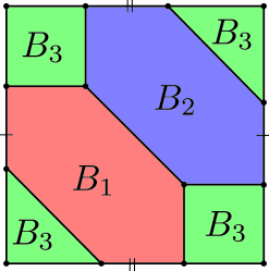
In this section we review the construction of a trisection of in [10]. Let . First, we consider the decomposition of . We can decompose any closed surface into three disks.
Lemma 3.1 (Lemma 3.1 in [10]).
admits a decomposition satisfies the following:
-
(1)
Each are disks,
-
(2)
is disjoint arcs.
-
(3)
is disjoint vertices.
If , this decomposition is illustrated in Figure 1. To obtain the case of a higher genus, remove a neighborhood of a vertex and glue a copy of it to itself along their boundary.
We take mutually disjoint disks in for . Then we define the 1-handlebodies of a trisection as follows:
To check is a 1-handlebody, we show that is a 1-handlebody. Since is a punctured genus surface, this can be represented by a disk and 1-handles attached to it. Since is a disk, is a 1-handlebody diffeomorphic to . The intersection and is a . This is a disjoint 3-balls in their boundaries. Since is a 4-ball, is a 1-handlebody of genus .
In [10], Williams showed that is a trisection.
Theorem 3.2 (Theorem 3.3 in [10]).
is a genus trisection.
The direction of this paper involves examining the above trisection in more detail to demonstrate how it will become a Weinstein trisection. To show this, we consider the Weinstein structure of and . This is constructed in Section 5. It is easy to show that each of is mutually ambient isotopic since they are disjoint disks. Also, we can show that each of is mutually ambient isotopic. Actually, in Figure 1, is sent to by ambient isotopy along the diagonal from bottom-left to top-right. We can extend this ambient isotopy to an arbitrary genus since we can construct a decomposition of by connecting summing a torus by taking the regular neighborhood of a vertex depicted in Figure 1. We consider this feature with a symplectic structure in the next subsection.
3.1. symplectomorphisms compatible to the trisection.
In this subsection, we see the self-symplectomorphisms of symplectic surfaces. First of all, we provide a definition of symplectic and Hamiltonian isotopy. Let be a closed symplectic manifold and a smooth function on . Then there is a unique vector field such that
since is non-degenerate. We call a Hamiltonian vector field associated to the Hamlltonian function .
Definition 3.3.
Let be an ambient isotopy on . We say is symplectic isotopy if is symplectomorphism for every .
A symplectic isotopy is called a Hamiltonian isotopy if is exact 1-form (i.e. is Hamiltonian vector field for every ) where is a vecotor field such that
By definition, a Hamiltonian isotopy is a symplectic isotopy.
In Section 5, we use the following lemmas to construct Weinstein structures of and .
To show Lemma 3.5, we use the following lemma.
Lemma 3.4 (cf. [8], P.113).
Let be a symplectic closed surface and a standard disk with radius for some .
be a smooth map such that is a symplectic embedding for every . Then there exists a Hamiltonian isotopy
such that
for all .
Lemma 3.5.
Let be a decomposition as in Lemma 3.1 and a symplectic form of . Suppose that each area of is identical for with respect to . Then there exists a symplectomorphism such that .
Proof.
Let be a ambient isotopy, such that
Let be a point in the interior of . Then, is a point in the interior of . Then we can construct a symplectic embedding so that
where is a smooth function on for . Then, we perturb so that for and any , we obtain the follwoing family of symplectic embeddings such that
From the result below, We can also assume that the in are sent to each other by symplectomorphism.
Lemma 3.6 (Theorem A in [1]).
Let be a symplectic closed surface and and are two sets of distinct points of . Then there is a symplectomorphism such that for that is isotopic to identity by an isotopy which preserves the structure and leaves fixed every point of outside a compact set of arbitrarily small volume.
4. Stein and Weinstein structure and Riemann surface.
4.1. Stein structure of a Riemann surface
We will review the concepts of Stein domains and that of Riemann surfaces. A Riemann surface is a 2-manifold with a complex structure . A Stein manifold is a complex manifold that is embedded in , where is a natural number. Grauert provided a characterization of Stein manifolds based on the function they admit (refer to [4]). This function is known as a strictly plurisubharmonic or -convex function. In the context of a smooth function , we say that it is exhausting if it is both proper and bounded from below.
Definition 4.1.
Let be a complex manifold and a function. is called a plurisubharmonic or -convex function if the 2-form
satisfies
for every non-zero tangent vector .
It is well-known that a Riemann surface is a Stein manifold if and only if it is a non-compact. Hence, becomes a Stein domain where is genus closed surface removed disks. Hence we obtain the following:
Lemma 4.2.
Let and be surfaces with genera and respectively, and and for are disks in and respectively that are defined in Section 3. Then, and will be Stein domains for .
4.2. Weinstein structure of Riemann surface
Liouville vector field on symplectic manifold is a vector field such that . If the Lie derivative of along is , then is a Liouville vector field. This follows from is closed. Liouville domain is the symplectic manifold with some compatible vector fields with contact boundaries.
Definition 4.3.
Let be a compact symplectic manifold with no empty boundary. is called a Liouville domain if there is a Liouville vector field defined globally and it is transversally out of the boundary. We denote it by
If the Liouville domain has a ”compatible” Morse function, it is called a Weinstein domain.
Definition 4.4.
Let be a Liouville domain. is called a Weinstein domain if there exists a Morse function it is locally constant in and is gradient-like for .
For a given symplectic manifold, it is difficult to determine whether it admits a Weinstein structure or not. Also, generally, it is difficult to construct a Weinstein structure but we sometimes construct it from a Stein structure.
We say exhausting J-convex function is completely exhausting if its gradient vector fields is complete where is a gradient respect to a Riemann metric for . The following is a well-known theorem:
Theorem 4.5 ([2]).
Let be a Stein manifold and a completely exhausting -convex Morse function. Then,
is a Weinstein structure on .
Hence, we can construct a Weinstein structure of from a Morse -convex function for .
5. Proof of the main theorem
Let us consider a 1-handlebody
that constructs a trisection prescribed in Section 3. We show that each of admits a Weinstein structure with respect to a symplectic structure defined by a product structure of .
Let be a -convex function such that contains only one critical point and its index is . Then we define the symplectic structure on so that
By Lemma 3.5, there is a symplectomorphism such that . Then we define the -convex function and as follows:
Then we can define the Weinstein structures on for by Theorem 4.5.
Let be a sufficiently small disk in and a -convex function. Also, we suppose that is a sufficiently small regular neighborhood of index critical point of and a disk in the interior of . Then we define the symplectic structure of so that
By Lemma 3.6, we can obtain the symplectomorphism such that
Then, we obtain the convex function as follows:
Also, we can obtain a symplectomorphism such that
by Lemma 3.6. Then, we can define the -convex function as follows:
Finally, we can construct a Weinstein structure on for by Theorem 4.5.
Proof of Theorem 1.1.
Let be a trivial bundle over surface with symplectic structure that is defined above. Now, the function is a -convex Morse function of . So, we have to show that the gradient vector field of this Morse function is outward and it is a Liouville vector field on with respect to a symplectic structure . Let be the gradient vector field of .
First, we show that is a Liouville vector field on with respect to . Now, and are -convex Morse function, and and are symplectic structure defined by and respectively. Hence, by Theorem 4.5, gives a Liouville vector fields on , particularly on for .
Next, we show that is transverse outwardly on the boudary of . we recall that
Since and intersects their boundaries, can be desicribed as following:
We note that . Then, we will see whether is outward for each region. We note that is a neighborhood of an index critical point of by definition of . Then, the restriction of to is transverse outwardly on its boundary. Since the restriction of to and is transverse outwardly on its boundary, transverse outwardly on and .
We note that is a neighborhood of an index critical point of by definition of . transverse outwardly on except since the restriction of to transeverse outwardly on except . But we see that
Hence the region is not included a boundary of . Hence transverse outwardly on entirely.
∎
6. The case where .
In this section, we give an example of the Weinstein trisection of . It is a trivial bundle over . We denote it . Also, has a decomposition described above. More precisely, we assume that is decomposed into three disks , , and as in Figure 1. We note that the Weinstein trisection of is constructed in former articles [7]. But in this section, we will describe it slightly more explicitly.
We construct a Weinstein trisection of as the following steps:
-
Step 1:
For a given symplectic structure on , we define a Morse function so that is a neighborhood of index critical point of , it does not contain the other critical point and whose gradient flow is a Liouville vector field of the symplectic structure. Furthermore, each of is mutually symplectically isotopic to each other.
-
Step 2:
For a given symplectic structure on , we define a Morse function so that is a neighborhood of index critical point of and does not contain the other critical points of , is a neighborhood of index critical point of and does not contain the other critical points of and whose gradient vector field is a Liouville vector field for the symplectic structure. Furthermore, each of is mutually symplectically isotopic to each other.
-
Step 3:
is a Morse function on and a gradient vector field of it is a Liouville vector field for the products of the symplectic structure of and and will be a Weinstein domain.
To begin the steps above, we review the Kähler structure on . First of all, we review the Fubini-study form of .
Let be a homogenious coordinate of . Then we can take a chart of by taking for
We denote this chart by . Then we define the Fubini-Study form by
where . It is known that this form gives us the Kähler form on , and in this case, gives a Kähler potential. The critical point of is only . This means that since . Also, we note that this is a -holomorphic function on . Hence, is a Stein manifold with -holomorphic function .
Next, we review the identification between and . We denote the polar coordinate of the unit sphere by the following (See Figure 2):
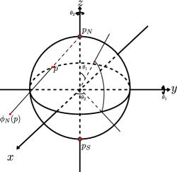
Then we can represent a point on by . We denote the stereographic projection where . Then we can define the diffeomorphism by
where . We sometimes use this diffeomorphism to define the function on below.
We identify and by and respectively.
6.1. Step 1: Weinstein structure on
We define the region , and on . Let be a -rotation along a -axis. Then we denote , and . Also, we denote , and . Then we define as a neighborhood of so that it contains and does not contain and for . and are defined by and respectively (See Figure 3).
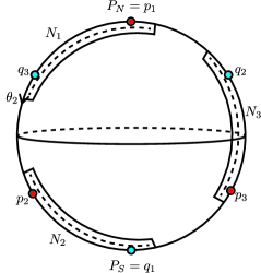
We take rotation along a such that is an empty set. Also, the we define and . Since a rotation is volume-preserving, this is a sympelctomorphism that sends to each other. Then define the -convex function on respect to . By using Theorem 4.5, we can obtain the Weinstein structure on . By permuting by rotation, we can also obtain the Weinstein structure on for .
6.2. Step 2: Weinstein structure on
We define the region in for as in Lemma 1. In this case, the intersection for is an arc. We define the region as follows:
We can see each region as in Figure 4.
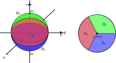
It is easy to see that each of is mutually permuted by rotating along a -axis. Also, we can define the -holomorphic function respect to on from the function defined above. Also, composing a and rotating, we can also obtain the -convex function on for . We will check that the critical point of is included in .
is a restriction of to it was defined before the steps. Its critical point is . This is corresponds to a point by the identification map . Also, this critical point has an index since by Poincare-Hopf theorem, is a Morse function on disk and it has only one critical point. Hence we can assume is a neighborhood of index critical point of .
6.3. Step 3: is a Weinstein domain.
We remain the following: First, we have to check the gradient flow of is the Liouville vector field. Next, we have to check it is outward. By Theorem 4.5, we can see that the gradient-like flow of and are Liouville vector fields with respect to . Hence we can show that the gradient-like flow of is a Liouville vector field with respect to .
Finally, we will check it is outward. Following the construction of trisection above, is a set as follows:
We show the case where . We note that each of and are diffeomorphic to a 4-ball since is a disk. We defined the vector field on and by the gradient-like vector field of and respectively. They are outward on each of and respectively. We denote an arc . Then the intersection of two 4-ball and is a 3-ball . We shall consider the boundary of . is a union of and . Now, the gradient-like vector field of on outward since and are neiborhood of index critical point of and respectively. Also, the gradient-like vector field of on is outward except since we can assume that is a neighborhood of index critical point of and the gradient-like vector field of is outward on . This is enough to show that is outward on .
7. Acknowledgement
The author thanks Takahiro Oba for a very meaningful discussion and suggestion about research in symplectic topology, also giving comments on a draft of this paper.
References
- [1] William M. Boothby, Transitivity of the automorphisms of certain geometric structures, Trans. Am. Math. Soc. 137 (1969), 93-100.
- [2] Y. Eliashberg and M. Gromov, Convex Symplectic Manifolds, Proceedings of Symposia in Pure Mathematics, 52, Part 2, 135-162 (1991).
- [3] D. Gay and R. Kirby. Trisecting 4-manifolds. Geom. Topol. 20 (2016), no. 6, 3097-3132.
- [4] H. Grauert and R. Remmert, Theory of Stein Spaces, Grundlehren der Mathematischen Wissenschaften 236, Springer-Verlag, Berlin (1979).
- [5] Lambert-Cole. Bridge trisections in and the Thom conjecture. Geom. Topol, 24(3) (2020), 1571-1614.
- [6] Lambert-Cole. Symplectic surfaces and bridge position. Geometriae Dedicata, 217(1) (2023) p.8.
- [7] P. Lambert-Cole, J.Meier, L.Starkston Symplectic 4‐manifolds admit Weinstein trisections. Journal of Topology. 2021 Jun;14(2):641-73.
- [8] D. McDuff and D. Salamon, Introduction to symplectic topology. Oxford University Press, (2017).
- [9] A. Weinstein. Contact surgery and symplectic handlebodies. Hokkaido Mathematical Journal, 20(2) (1991), pp.241-251.
- [10] M. Williams. Trisections of flat surface bundles over surfaces Doctoral Thesis, The University of Nebraska-Lincoln (2020).