Weighted Distillation with Unlabeled Examples

Fotis Iliopoulos
Google Research
[email protected]
Vasilis Kontonis
Google Research
[email protected]
Cenk Baykal
Google Research
[email protected]
Gaurav Menghani
Google Research
[email protected]
Khoa Trinh
Google Research
[email protected]
Erik Vee
Google Research
[email protected]

Abstract

Distillation with unlabeled examples is a popular and powerful method for training deep neural networks in settings where the amount of labeled data is limited: A large “teacher” neural network is trained on the labeled data available, and then it is used to generate labels on an unlabeled dataset (typically much larger in size). These labels are then utilized to train the smaller “student” model which will actually be deployed. Naturally, the success of the approach depends on the quality of the teacher’s labels, since the student could be confused if trained on inaccurate data. This paper proposes a principled approach for addressing this issue based on a “debiasing" reweighting of the student’s loss function tailored to the distillation training paradigm. Our method is hyper-parameter free, data-agnostic, and simple to implement. We demonstrate significant improvements on popular academic datasets and we accompany our results with a theoretical analysis which rigorously justifies the performance of our method in certain settings.

1 Introduction

In many modern applications of deep neural networks, where the amount of labeled examples for training is limited, distillation with unlabeled examples [8, 20] has been enormously successful. In this two-stage training paradigm a larger and more sophisticated “teacher model” — typically non-deployable for the purposes of the application — is trained to learn from the limited amount of available training data in the first stage. In the second stage, the teacher model is used to generate labels on an unlabeled dataset, which is usually much larger in size than the original dataset the teacher itself was trained on. These labels are then utilized to train the “student model”, namely the model which will actually be deployed. Notably, distillation with unlabeled examples is the most commonly used training-paradigm in applications where one finetunes and distills from very large-scale foundational models such as BERT [13] and GPT-3 [5] and, additionally, it can be used to significantly improve distillation on supervised examples only (see e.g. [47]).

While this has proven to be a very powerful approach in practice, its success depends on the quality of labels provided by the teacher model. Indeed, often times the teacher model generates inaccurate labels on a non-negligible portion of the unlabeled dataset, confusing the student. As deep neural networks are susceptible to overfitting to corrupted labels [50], training the student on the teacher’s noisy labels can lead to degradation in its generalization performance. As an example, Figure 1 depicts an instance based on CIFAR-10 where filtering out the teacher’s noisy labels is quite beneficial for the student’s performance.

We address this shortcoming by introducing a natural “noise model” for the teacher which allows us to modify the student’s loss function in a principled way in order to produce an unbiased estimate of the student’s clean objective. From a practical standpoint, this produces a fully “plug-and-play” method which adds minimal implementation overhead, and which is composable with essentially every other known distillation technique.

The idea of compressing a teacher model into a smaller student model by matching the predictions of the teacher was initially introduced by Buciluǎ, Caruana and Niculescu-Mizil [6] and, since then, variations of this method [20, 26, 31, 35, 39, 42, 49] have been applied in a wide variety of contexts [37, 48, 51]. (Notably, some of these applications go beyond compression — see e.g. [8, 47, 48, 52] for reference.) In the simplest form of the method [26], and using classification as a canonical example, the labels produced by the teacher are one-hot vectors that represent the class which has the maximum predicted probability — this method is often referred to as “hard”-distillation. More generally, Hinton et. al. [8, 20] have shown that it is often beneficial to train the student so that it minimizes the cross-entropy (or KL-divergence) with the probability distribution produced by the teacher while also potentially using a temperature higher than $1$ in the softmax of both models (“soft”-distillation). (Temperatures higher than $1$ are used in order to emphasize the difference between the probabilities of the classes with lower likelihood of corresponding to the correct label according to the teacher model.)

The main contribution of this work is a principled method for improving distillation with unlabeled examples by reweighting the loss function of the student. That is, we assign importance weights to the examples labeled by the teacher so that each weight reflects (i) how likely it is that the teacher has made an inaccurate prediction regarding the label of the example and (ii) how “distorted” the unweighted loss function we use to train the student is (measured with respect to using the ground-truth label for the example instead of the teacher’s label). More concretely, our reweighting strategy is based on introducing and analyzing a certain noise model designed to capture the behavior of the teacher in distillation. In this setting, we are able to come up with a closed-form solution for weights that “de-noise” the objective in the sense that (on expectation) they simulate having access to clean labels. Crucially, we empirically observe that the key characteristics of our noise model for the teacher can be effectively estimated through a small validation dataset, since in practice the teacher’s noise is neither random nor adversarial, and it typically correlates well with its “confidence” — see e.g. Figure 1. In particular, we use the validation dataset to learn a map that takes as input the teacher’s and student’s confidence for the label of a certain example and outputs estimates for the quantities mentioned in items (i) and (ii) above. Finally, we plug in these estimates to our closed-form solution for the weights so that, overall, we obtain an automated way of computing the student’s reweighted objective in practice. A detailed description of our method can be found in Section 2.3.

Our main findings and contributions can be summarized as follows:

•

We propose a principled and hyperparameter-free reweighting method for knowledge distillation with unlabeled examples. The method is efficient, data-agnostic and simple to implement.
•

We present extensive experimental results which show that our method provides significant improvements when evaluated in standard benchmarks.
•

Our reweighting technique comes with provable guarantees: (i) it is information-theoretically optimal; and (ii) under standard assumptions SGD optimization of the reweighted objective learns a solution with nearly optimal generalization.

Refer to caption — Figure 1: Left: Performance comparison between a student trained using conventional distillation with unlabeled examples (orange) and a student trained only on the examples which are labeled *correctly* by the teacher (blue). Here we assume access to $7500$ labeled examples and $40500$ unlabeled examples of CIFAR-10. The teacher is a MobileNet of depth multiplier $2$ , while the student is a MobileNet of depth multiplier $1$ . Right: Plot of teacher’s accuracy as a function of the margin score.

1.1 Related work

Fidelity vs Generalization in knowledge distillation. Conceptually, our work is related to the paper of Stanton et al. [43] where the main message is that “good student accuracy does not imply good distillation fidelity”, i.e., that more closely matching the teacher does not necessarily lead to better student generalization. In particular, [43] demonstrates that when it comes to enlarging the distillation dataset beyond the teacher training data, there is a trade-off between optimization complexity and distillation data quality. Our work can be seen as a principled way of improving this trade-off.

Advanced distillation techniques. Since the original paper of Hinton et. al. [20], there have been several follow-up works [2, 7, 31, 45] which develop advanced distillation techniques which aim to enforce greater consistency between the teacher and the student (typically in the context of distillation on labeled examples). These methods enforce consistency not only between the teacher’s predictions and student’s predictions, but also between the representations learned by the two models. However, in the context of distillation with unlabeled examples, forcing the student to match the teacher’s inaccurate predictions is still harmful, and therefore weighting the corresponding loss functions via our method is still applicable and beneficial. We demonstrate this fact by considering instances of the Variational Information Distillation for Knowledge Transfer (VID) [2] framework, and showing how it is indeed beneficial to combine it with our method in Section 3.1.3. We also show that our approach provides benefits on top of any improvement obtained via temperature-scaling in Appendix B.2.

Learning with noisy data techniques. As we have already discussed, the main conceptual contribution of our work is viewing the teacher model in distillation with unlabeled examples as the source of stochastic noise with certain characteristics. Naturally, one may wonder what is the relationship between our method and works from the vast literature of learning with noisy data (e.g. [4, 14, 16, 23, 25, 27, 29, 33, 36, 38]). The answer is that our method does not attempt to solve the generic “learning with noisy data” problem, which is a highly non-trivial task in the absence of assumptions (both in theory and in practice). Instead, our contribution is to observe and exploit the fact that the noise introduced by the teacher in distillation has structure, as it correlates with several metrics of confidence such as the margin-score, the entropy of the predictions etc. We use and quantify this empirical observation to our advantage in order to formulate a principled method for developing a debiasing reweighting scheme (an approach inspired by the “learning with noisy data"-literature) which comes with theoretical guarantees. An additional difference is that works from the learning with noisy data literature typically assume that the training dataset consists of corrupted hard labels, and often times their proposed method is not compatible with soft-distillation (in the sense that they degrade its performance, making it much less effective) — see e.g. [32] for a study of this phenomenon in the case of label smoothing [28, 44].

Uncertainty-based weighting schemes. Related to our method are approaches for semi-supervised learning where examples are downweighted or filtered out when the teacher is “uncertain.” (A plethora of ways for defining and measuring “uncertainty” have been proposed in the literature, e.g. entropy, margin-score, dropout variance etc.) These methods are independent of the student model (they only depend on the teacher model), and so they cannot hope to remove the bias from the student’s loss function. In fact, these methods can be viewed as preprocessing steps that can be combined with the student-training process we propose. To demonstrate this we both combine and compare our method to the fidelity-based weighting scheme of [12] in Section 3.3.

1.2 Organization of the paper.

In Section 2, we present our method in detail, while in Section 3 we present our key experimental results. In Section 4, we discuss the theoretical aspects of our work. In Section 5, we summarize our results, we discuss the benefits and limitations of our method, and future work. Finally, we present extended experimental and theoretical results in the Appendix.

2 Weighted distillation with unlabeled examples

In this section we present our method. In Section 2.1, we review multiclass classification. In Section 2.2, we introduce the noise model for the teacher in distillation, which motivates our approach. And finally, in Section 2.3, we describe our method in detail.

2.1 Multiclass classification

In multiclass classification, we are given a training sample $S=\{(x_{1},y_{1}),(x_{2},y_{2}),\ldots(x_{n},y_{n})\}$ drawn from $\mathbb{P}^{n}$ , where $\mathbb{P}$ is an unknown distribution over instances $\mathcal{X}$ and labels $\mathcal{Y}=[L]=\{1,2,\ldots,L\}$ . Our goal is to learn a predictor $f:\mathcal{X}\rightarrow\mathbb{R}^{L}$ , namely to minimize the risk of $f$ . The latter is defined as the expected loss of $f$ :

\displaystyle R(f)={\mathbb{E}}[\ell(y,f(x))]

(1)

where $(x,y)$ is drawn from $\mathbb{P}$ , and $\ell:[L]\times\mathbb{R}^{L}\rightarrow\mathbb{R}_{+}$ is a loss function such that, for a label $y\in[L]$ and prediction vector $f(x)\in\mathbb{R}^{L}$ , $\ell(y,f(x))$ is the loss incurred for predicting $f(x)$ when the true label is $y$ . The most common way to approximate the risk of a predictor $f$ is via the so-called empirical risk:

\displaystyle R_{S}(f)=\frac{1}{|S|}\sum_{(x,y)\in S}\ell(y,f(x)).

(2)

That is, given a hypothesis class of predictors $\mathcal{F}$ , our goal is typically to find $\min_{f\in\mathcal{F}}R_{S}(f)$ as a way to estimate $\min_{f\in\mathcal{F}}R(f)$ .

2.2 Debiasing weights

As we have already discussed, the main drawback of distillation with unlabeled examples is essentially that the empirical risk minimizer corresponding to the dataset labeled by the teacher cannot be trusted, since the teacher may generate inaccurate labels. To quantify this phenomenon and guide our algorithmic design, we consider the following simple but natural noise model for the teacher.

Let $\mathbb{X}$ be an unknown distribution over instances $\mathcal{X}$ . We assume the existence of a ground-truth classifier so that each $x\in\mathcal{X}$ is associated with a ground-truth label $f_{\mathrm{true}}(x)\in[L]=\{1,2,\ldots,L\}$ . In other words, a clean labeled example is of the form $(x,f_{\mathrm{true}}(x))\sim\mathbb{P}$ (and $x\sim\mathbb{X}$ ). Additionally, we consider a stochastic adversary that given an instance $x\in\mathcal{X}$ , outputs a “corrupted” label $y_{\mathrm{adv}}(x)$ with probability $p(x)$ , and the ground-truth label $f_{\mathrm{true}}(x)$ with probability $1-p(x)$ . Let $\mathbb{D}$ denote the induced adversarial distribution over instances and labels.

It is not hard to see that the empirical risk with respect to a predictor $f$ and sample from $\mathbb{D}$ is not an unbiased estimator of the risk

\displaystyle R(f)={\mathbb{E}}_{x\sim\mathbb{X}}[\ell(f_{\mathrm{true}}(x),f(x))]

(3)

— see Proposition 2.1. On the other hand, the following weighted empirical risk (5) is indeed an unbiased estimator of $R(f)$ . For each $x\in\mathcal{X}$ let

\displaystyle w_{f}(x)=\frac{1}{1+p(x)\left(\mathrm{distortion}_{f}(x)-1\right)},\leavevmode\nobreak\ \leavevmode\nobreak\ \leavevmode\nobreak\ \text{where}\leavevmode\nobreak\ \leavevmode\nobreak\ \leavevmode\nobreak\ \mathrm{distortion}_{f}(x)=\frac{\ell(y_{\mathrm{adv}}(x),f(x))}{\ell(f_{\mathrm{true}}(x),f(x))},

(4)

and define

\displaystyle R_{S}^{w}(f)=\frac{1}{|S|}\sum_{(x,y)\in S}w_{f}(x)\,\ell(y,f(x)),

(5)

where $S=\{(x_{i},y_{i})\}_{i=1}^{n}\sim\mathbb{D}^{n}$ . Observe that the weight for each instance $x$ depends on (i) how likely it is the adversary corrupts its label; and on (ii) how this corrupted label “distorts” the loss we observe at instance $x$ . In the following proposition we establish that the standard (unweighted) empirical risk with respect to distribution $\mathbb{D}$ and a predictor $f$ is a biased estimator of the risk of $f$ under the clean distribution $\mathbb{P}$ , while the weighted empirical risk (5) is an unbiased one.

Proposition 2.1 (Debiasing Weights).

Let $S=\{(x_{i},y_{i})\}_{i=1}^{n}\sim\mathbb{D}^{n}$ be a sample from the adversarial distribution. Defining $\mathrm{Bias}(f)={\mathbb{E}}_{x\sim\mathbb{X}}\left[p(x)\cdot(\mathrm{distortion}_{f}(x)-1)\cdot\ell(f_{\mathrm{true}}(x),f(x))\right]$ we have:

\displaystyle\text{``reweighted''}\leavevmode\nobreak\ \leavevmode\nobreak\ \leavevmode\nobreak\ {\mathbb{E}}[R_{S}^{w}(f)]=R(f)\leavevmode\nobreak\ \leavevmode\nobreak\ \leavevmode\nobreak\ \leavevmode\nobreak\ \leavevmode\nobreak\ \leavevmode\nobreak\ \text{vs}\leavevmode\nobreak\ \leavevmode\nobreak\ \leavevmode\nobreak\ \leavevmode\nobreak\ \leavevmode\nobreak\ \leavevmode\nobreak\ \text{``standard''}\leavevmode\nobreak\ \leavevmode\nobreak\ \leavevmode\nobreak\ {\mathbb{E}}[R_{S}(f)]

\displaystyle=R(f)+\mathrm{Bias}(f)\,.

Notice that, as expected, the bias of the unweighted predictor is a function of the “power” of the adversary, i.e., a function of how often they can corrupt the label of an instance, and the “distortion” this corruption causes to the loss we observe. The proof of Proposition 2.1 follows from simple, direct calculations and it can be found in Appendix D.3.

Intuitively, given a sufficiently large sample $S\sim\mathbb{D}^{n}$ , optimizing an unbiased estimator for the risk should provide a better approximation for $\min_{f\in F}R(f)$ compared to optimizing an estimator with constant bias. We formalize this intuition in Section 4 and in Appendix D.

2.3 Our method

We consider the standard setting for distillation with unlabeled examples where we are given a dataset $S_{\ell}=\{(x_{i},y_{i})\}_{i=1}^{m}$ of $m$ labeled examples from an unknown distribution $\mathbb{P}$ , and a dataset $S_{u}=\{x_{i}\}_{i=m+1}^{m+n}$ of $n$ unlabeled examples — typically, $n\geq m$ . We also assume the existence of a (small) clean validation dataset $S_{v}=\{(x_{i},y_{i})\}_{i=m+n+1}^{i=m+n+q}$ of size $q$ . Finally, let $\ell:\mathbb{R}^{L}\times\mathbb{R}^{L}\rightarrow\mathbb{R}_{+}$ be a loss function that takes as input two vectors over the set of labels $[L]$ . We describe our method below and more formally in Algorithm 1 in Appendix A.

Remark 2.1.

The only assumption we need to make about the validation set $S_{v}$ is that it is not in the train set of the teacher model. That is, set $S_{v}$ can be used in the train set of the student model if needed — we chose to present $S_{v}$ as a completely independent hold out set to make our presentation as conceptually clear as possible.

Training the teacher. The teacher model is trained on dataset $S_{\ell}$ , and then it is used to generate labels for the instances in $S_{u}$ . The labels can be one-hot vectors or probability distributions on $[L]$ , depending on whether we apply “hard” or “soft” distillation, respectively.

Training the student. We start by pretraining the student model on dataset $S_{\ell}$ . Then, the idea is to think of the teacher model as the source of noise in the setting of Section 2.2, compute a weight $w_{f}(x)$ for each example $x$ based on (4), and finally train the student on the union of labeled and teacher-labeled examples by minimizing the weighted empirical risk (examples from $S_{\ell}$ are assigned unit weight).

We point out two remarks. First, in order to apply (4) to compute the weight of an example $x$ , we need to have estimates of $p(x)$ and $\mathrm{distortion}_{f}(x)$ . To obtain these estimates we use the validation dataset $S_{v}$ as we describe in the next paragraph. Second, observe that, according to (4), the weight of an example is a function of the predictor, namely the parameters of the model in the case of neural networks. This means that ideally we should be updating our weights assignment every time the parameters of the student model get updated during training. However, we empirically observe that even estimating the weight assignment only once during the whole training process (right after training the student model on $S_{\ell}$ ) suffices for our purposes, and so our method adds minimal overhead to the standard training process. More generally, the fact that our process of computing the weights is simple and inexpensive allows us to recompute them during training (say every few epochs) to improve our approximation of the theoretically optimal weights. We explore the effect of updating the weights during training in Section 3.2.

Estimating the weights. We estimate the weights using the Nearest Neighbors method on $S_{v}$ to learn a map that takes as input the teacher’s and student’s “confidence” for the label of a certain example $x$ , and outputs estimates for $p(x)$ and $\mathrm{distortion}_{f}(x)$ so we can apply (4). In our experiments we measure the confidence of a model either via the margin-score, i.e., the difference between the largest two predicted classes for the label of a given example (see e.g. the so-called “margin” uncertainty sampling variant [40]), or via the entropy of its prediction. However, one could use any metric (not necessarily confidence) that correlates well with the accuracy of the corresponding models.

More concretely, we reduce the task of estimating the weights to a two-dimensional (i.e., two inputs and two outputs) regression task over the validation set which we solve using the Nearest Neighbors method. In particular, our Nearest Neighbor data structure is constructed as follows. Each example $x$ of the validation set is assigned the two following pairs of points: (i) (teacher confidence at $x$ , student confidence at $x$ ) — this is the covariate of the regression task; (ii) ( $1$ , distortion at ( $x$ )) if the teacher correctly predicts the label of $x$ , or ( $0$ , distortion at $x$ ), if the teacher does not correctly predict the label of $x$ — this is the response of the regression task. The query corresponding to an unlabeled example $x^{\prime}$ is of the form (teacher confidence at $x^{\prime}$ , student confidence at $x^{\prime}$ ). The Nearest Neighbors data structure returns the average response over the $k$ closest in euclidean distance pairs (teacher confidence at $x$ , student confidence at $x$ ) in the validation set. The value of $k$ is specified in the next paragraph. The pseudocode for our method can be found in Algorithm 2 in Appendix A.

We point out two remarks. First, the number $k$ of neighbors we use for our weights-estimation is always $k=\frac{\sqrt{|S_{v}|}}{2}$ . This is because choosing $k=\Theta(q^{2/(2+\mathrm{dim})})$ , where $q$ is the size of the validation dataset and $\mathrm{dim}$ is the dimension of the underlying metric space ( $\mathrm{dim}=2$ in our case), is asymptotically optimal, and $1/2$ is a popular choice for the hidden constant used in practice, see e.g. [9, 18]. Second, notice that (4) implies that the weight of an example could be larger than $1$ if (and only if) the corresponding distortion value (4) at that example is less than $1$ . This could happen for example if both the student and teacher have the same (or very similar) inaccurate prediction for a certain example. In such a case, the value of the weight in (4) informs us that the loss at this example should be larger than the (low) value the unweighted loss function suggests. However, since we do not have the ground-truth label for a point during training — but only the inaccurate prediction of the teacher — having a weight larger than $1$ in this case would most likely guide our student model to fit an inaccurate label. To avoid this phenomenon, we always project our weights onto the $[0,1]$ interval (Line 16 of Algorithm 2). In Appendix D.2 we discuss an additional reason why it is beneficial to project the weights of examples of low distortion onto $[0,1]$ based on a MSE analysis.

3 Experimental results

In this section we present our experimental results. In Section 3.1 we consider an experimental setup according to which the weights are estimated only once during the whole training process. In Section 3.2 we study the effect of updating the weights during training. Finally, in Section 3.3 we demonstrate that our method can be combined with uncertainty-based weighting techniques by both combining and comparing our method to the fidelity-based weighting scheme of [12].

3.1 Improvements via one-shot estimation of the weights

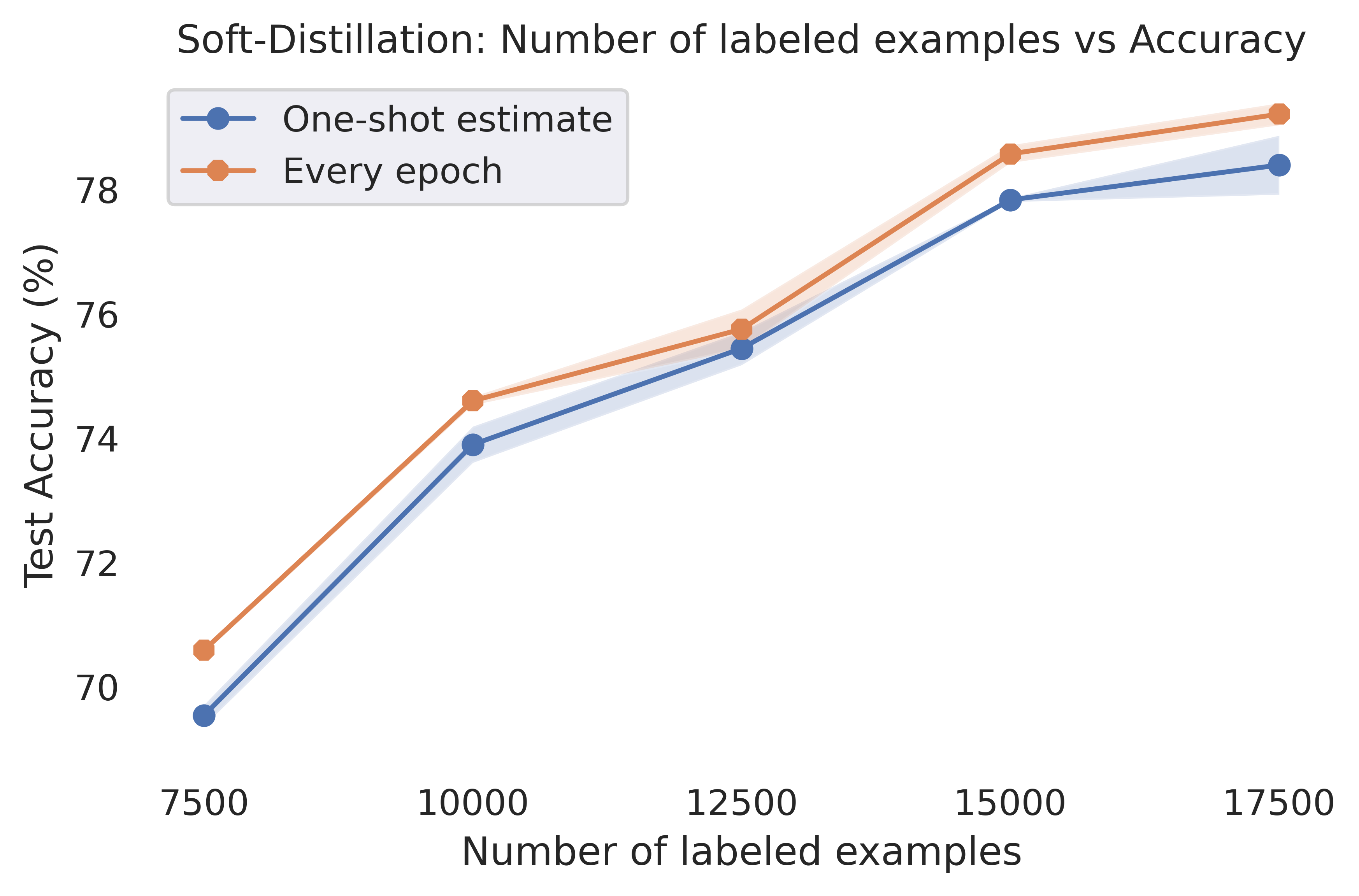
Here we show how applying our reweighting scheme provides consistent improvements on several popular benchmarks even when the weights are estimated only once during the whole training process. We compare our method against conventional distillation with unlabeled examples, but we also show that our method can provide benefits when combined with more advanced distillation techniques such as the framework of [2] (see Figure 9).

More concretely, we evaluate our method on benchmark vision datasets. We compare our method to conventional distillation with unlabeled examples both in terms of the best test accuracy achieved by the student, and in terms of convergence speed (see Figure 2). We also evaluate the comparative advantage of our method as a function of the number of labeled examples available (size of dataset $S_{\ell}$ ). We always choose the temperature in the softmax of the models to be $1$ for simplicity and consistency, and our metric for confidence is always the margin-score. Implementation details for our experiments and additional results can be found in Appendices B and C. We implemented all algorithms in Python making use of the TensorFlow deep learning library [1]. We use 64 Cloud TPU v4s each with two cores.

3.1.1 Experimental setup

Our experiments are of the following form. The academic dataset we use each time is first split into two parts $A$ and $B$ . Part $A$ , which is typically smaller, is used as the labeled dataset $S_{\ell}$ where the teacher model is trained on (recall the setting we described in Section 2.3). Part $B$ is randomly split again into two parts which represent the unlabeled dataset $S_{u}$ and validation dataset $S_{v}$ , respectively. Then, (i) the teacher and student models are trained once on the labeled dataset $S_{\ell}$ ; (ii) the teacher model is used to generate soft-labels for the unlabeled dataset $S_{u}$ ; (iii) we train the student model on the union of $S_{\ell}$ and $S_{u}$ using our method and conventional distillation with unlabeled examples. We repeat step (iii) a number of times: in each trial we partition part $B$ randomly and independently, and then the student model is trained using the (student-)weights reached after completing the training on dataset $S_{\ell}$ in step (i) as initialization, both for our method and the competing approaches.

3.1.2 CIFAR-{10, 100} and SVHN experiments

SVHN [34] is an image classification dataset where the task is to classify street view numbers ( $10$ classes). The train set of SVHN contains $73257$ labeled images and its test set contains $26032$ images. We use a MobileNet [21] with depth multiplier $2$ as the teacher, and a MobileNet with depth multiplier $1$ as the student¹¹1Note that we see the student outperform the teacher here and in other experiments, as can often happen with distillation with unlabeled examples, particularly when the teacher is trained on limited data.. The tables in Figure 4 contain the results of our experiments (averages over $3$ trials). In each experiment we use the first $N\in\{7500,10000,12500,15000,17500,20000\}$ examples as the labeled dataset $S_{\ell}$ , and then the rest $73257-N$ images are randomly split to a labeled validation dataset $S_{v}$ of size $2000$ , and an unlabeled dataset $S_{u}$ of size $71257-N$ .

CIFAR-10 and CIFAR-100 [24] are image classification datasets with $10$ and $100$ classes respectively. Each of them consists of $60000$ labeled images, which we split to a training set of $50000$ images, and a test set of $10000$ images. For CIFAR-10, we use a Mobilenet with depth multiplier $2$ as the teacher, and a Mobilenet with depth multiplier $1$ as the student. For CIFAR-100, we use a ResNet-110 as a teacher, and a ResNet-56 as the student. We use a validation set of $2000$ examples. The results of our experiments (averages over $3$ trials) can be found in the tables of Figures 5, 6.

Labeled Examples	$7500$	$10000$	$12500$	$15000$	$17500$
Teacher	$87.31\%$	$88.5\%$	$88.45\%$	$91.38\%$	$91.32\%$
Weighted (Ours)	$\mathbf{90.41\pm 0.12}\%$	$\mathbf{91.21\pm 0.09\%}$	$\mathbf{92.4\pm 0.12\%}$	$\mathbf{92.64\pm 0.14\%}$	$\mathbf{92.85\pm 0.1\%}$
Unweighted	$89.89\pm 0.09\%$	$90.86\pm 0.11\%$	$91.99\pm 0.1\%$	$92.51\pm 0.07\%$	$92.45\pm 0.07\%$

Figure 4: Experiments on SVHN. See Section 3.1.2 for details.

Labeled Examples	$7500$	$10000$	$12500$	$15000$	$17500$
Teacher	$67.17\%$	$71.39\%$	$74.69\%$	$77\%$	$78.46\%$
Weighted (Ours)	$\mathbf{69.01\pm 0.25}\%$	$\mathbf{72.96\pm 0.1\%}$	$\mathbf{75.33\pm 0.43\%}$	$\mathbf{77.69\pm 0.35\%}$	$\mathbf{78.34\pm 0.16\%}$
Unweighted	$68.27\pm 0.22\%$	$72.48\pm 0.26\%$	$74.95\pm 0.2\%$	$76.85\pm 0.32\%$	$77.92\pm 0.06\%$

Figure 5: Experiments on CIFAR-10. See Section 3.1.2 for details.

Labeled Examples	$7500$	$10000$	$12500$	$15000$	$17500$
Teacher	$44.1\%$	$51.31\%$	$55.54\%$	$59.05\%$	$62.17\%$
Weighted (Ours)	$\mathbf{46.81\pm 0.34}\%$	$\mathbf{53.31\pm 0.66\%}$	$\mathbf{57.5\pm 0.3}\%$	$\mathbf{60.94\pm 0.32\%}$	$\mathbf{62.86\pm 0.41\%}$
Unweighted	$46.29\pm 0.04\%$	$52.83\pm 0.53\%$	$56.89\pm 0.65\%$	$60.73\pm 0.03\%$	$62.79\pm 0.09\%$

Figure 6: Experiments on CIFAR-100. See Section 3.1.2 for details.

3.1.3 CelebA experiments: considering more advanced distillation techniques

As we have already discussed in Section 1.1, our method can be combined with more advanced distillation techniques which aim to enforce greater consistency between the teacher and the student. We demonstrate this fact by implementing the method of Variational Information Distillation for Knowledge Transfer (VID) [2] and showing how it is indeed beneficial to combine it with our method. We chose the gender binary classification task of CelebA [15] as our benchmark (see details in the next paragraph), because it is known (see e.g. [31]) that the more advanced distillation techniques tend to be more effective when applied to classification tasks with few classes. In the table below, “Unweighted VID” corresponds to the implementation of loss described in equations (2), (4) and (6) of [2], and “Weighted VID” corresponds to the reweighting of the latter loss using our method.

CelebA [15] is a large-scale face attributes dataset with more than $200000$ celebrity images, each with forty attribute annotations. Here we consider the binary male/female classification task. The train set of CelebA contains $162770$ images and its test set contains $19962$ images. We use a MobileNet with depth multiplier $2$ as the teacher, and a ResNet-11 [19] as the student. The tables in Figure 7 contain the results of our experiments (averages over $3$ trials). In each experiment we use the first $N\in\{10000,15000,20000,25000,30000,35000\}$ examples as the labeled dataset $S_{\ell}$ , and then the rest $162770-N$ images are randomly split to a labeled validation dataset $S_{v}$ of size $2000$ , and an unlabeled dataset $S_{u}$ of size $160770-N$ .

Labeled Examples	$10000$	$15000$	$20000$	$25000$	$30000$
Teacher	$91.59\%$	$93.76\%$	$94.41\%$	$94.86\%$	$94.92\%$
Weighted VID	$\mathbf{94.35\pm 0.11\%}$	$95.01\pm 0.17\%$	$\mathbf{95.73\pm 0.04\%}$	$\mathbf{95.89\pm 0.08}\%$	$\mathbf{96.11\pm 0.08\%}$
Weighted Conventional	$94.06\pm 0.04\%$	$\mathbf{95.14\pm 0.1\%}$	$95.56\pm 0.03\%$	$\mathbf{95.86\pm 0.03\%}$	$95.92\pm 0.01\%$
Unweighted VID [2]	$94.11\pm 0.11\%$	$94.76\pm 0.14\%$	$95.46\pm 0.11\%$	$95.69\pm 0.05\%$	$95.88\pm 0.03\%$
Unweighted Conventional	$93.68\pm 0.01\%$	$94.92\pm 0.02\%$	$95.38\pm 0.07\%$	$95.69\pm 0.05\%$	$95.73\pm 0.09\%$

Figure 7: Experiments on CelebA. See Section 3.1.3 for details and also Figure 3.

3.1.4 ImageNet experiments

ImageNet [41] is a large-scale image classification dataset with $1000$ classes consisting of approximately $I\approx 1.3$ M images. For our experiments, we use a ResNet-50 as the teacher, and a ResNet-18 as the student. In each experiment we use the first $N\in\{64058,128116\}$ labeled examples ( $5\%$ and $10\%$ of $I$ , respectively) as the labeled dataset $S_{\ell}$ , and the rest $I-N$ examples are randomly split to a labeled validation dataset $S_{v}$ of size $10000$ , and an unlabeled dataset $S_{u}$ of size $I-N-10000$ . The results of our experiments (averages over 10 trials) can be found in Figure 8.

Labeled Examples	$5\%$ of ImageNet	$10\%$ of ImageNet
Teacher (soft)	$36.74\%$	$51.88\%$
Weighted (Ours)	$\mathbf{38.60\pm 0.07}\%$	$\mathbf{53.59\pm 0.09}\%$
Unweighted	$38.44\pm 0.06\%$	$53.43\pm 0.08\%$

Labeled Examples	$5\%$ of ImageNet	$10\%$ of ImageNet
Teacher (hard)	$36.74\%$	$51.88\%$
Weighted (Ours)	$\mathbf{38.56\pm 0.07\%}$	$\mathbf{53.34\pm 0.11\%}$
Unweighted	$38.42\pm 0.06\%$	$53.18\pm 0.07\%$

Figure 8: Experiments with soft-distillation (left) and hard-distillation (right) on ImageNet.

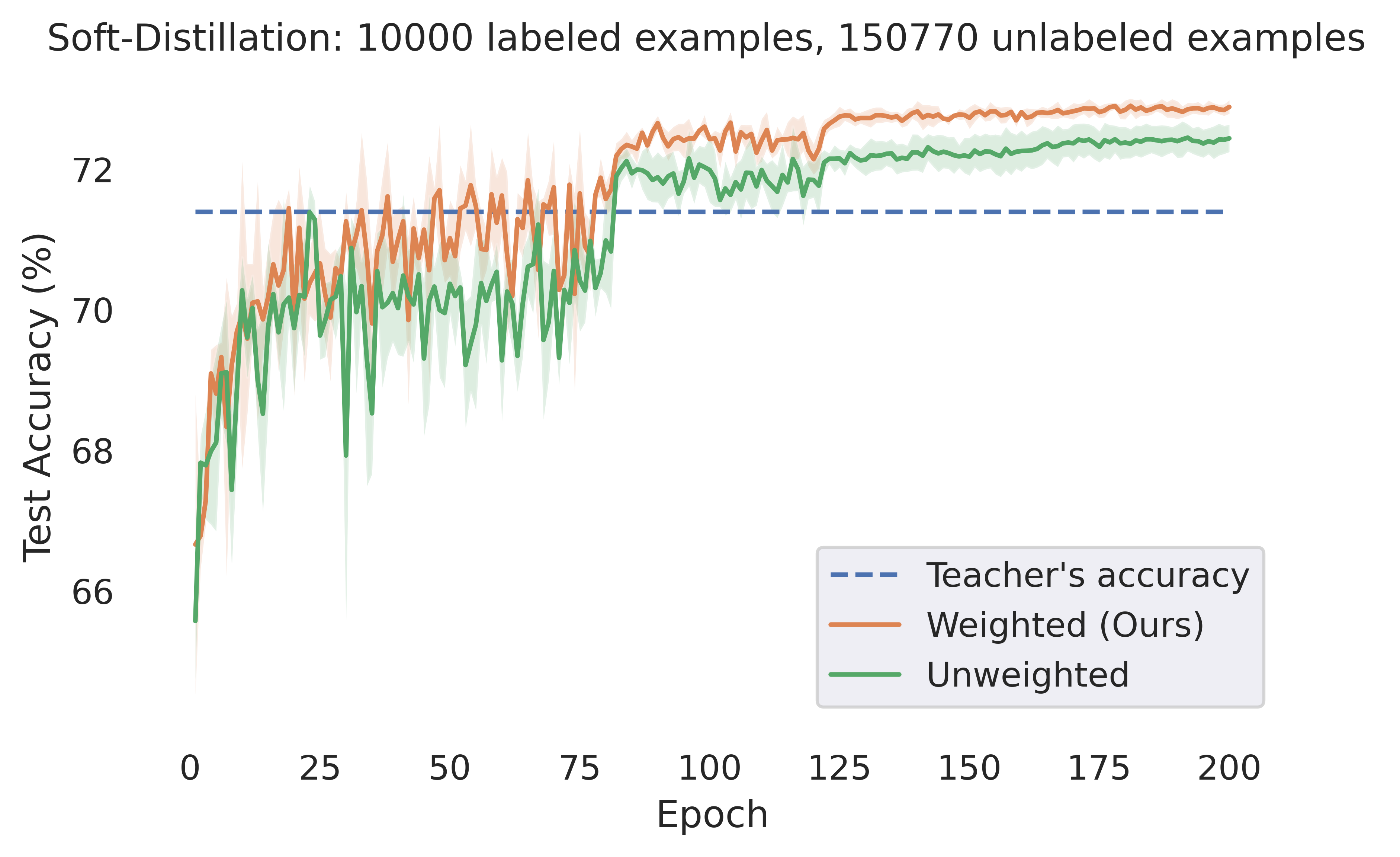
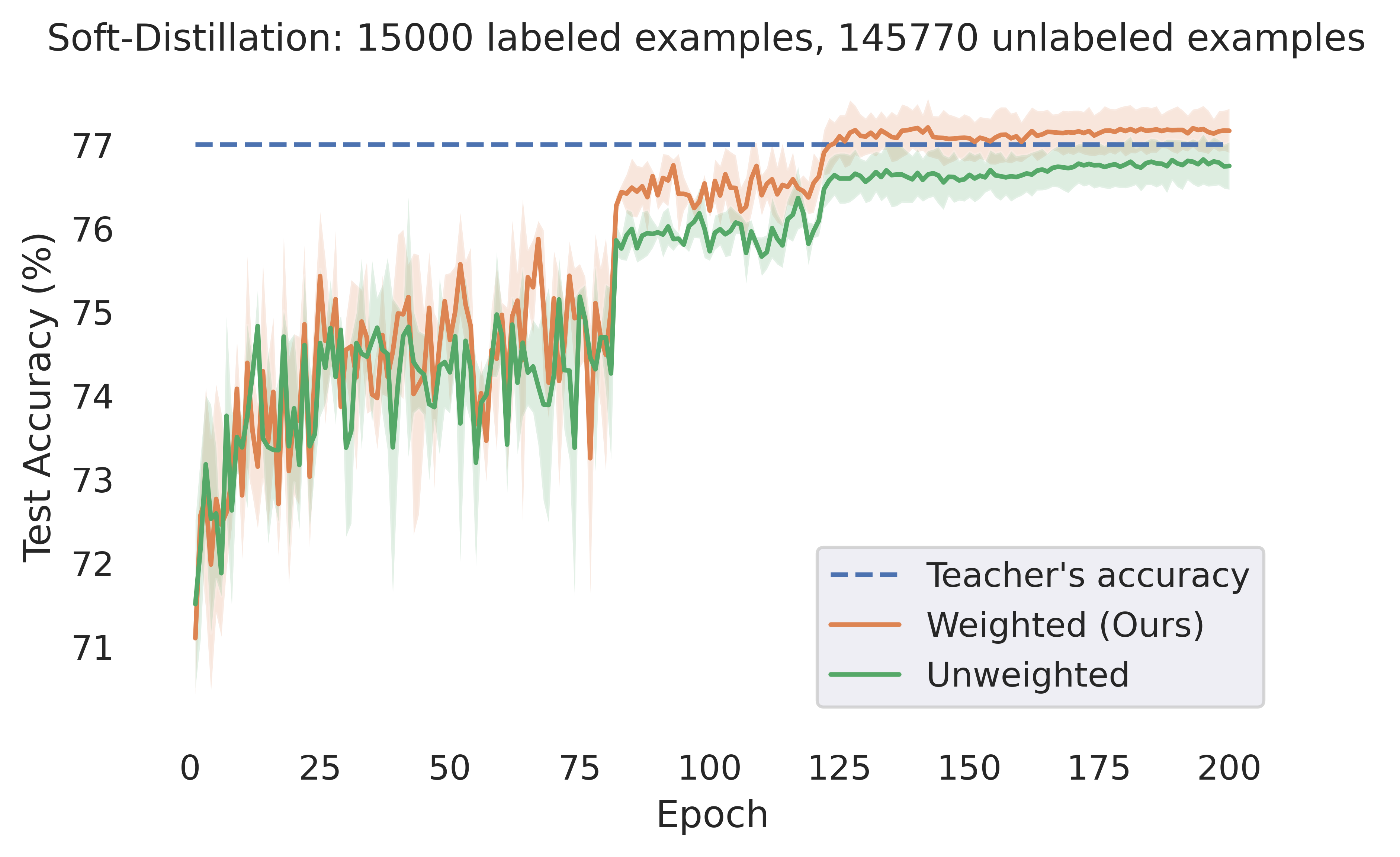
3.2 Updating the weights during training

In this section we consider the effect of updating our estimation of the optimal weights during training. For each dataset we consider, the experimental setup is identical to the corresponding setting in Section 3.1, except for that we always use a validation set of size $500$ and the entropy of a model’s prediction as the metric for its confidence. We note that the time required for computing the weight for each example is insignificant compared to total training time (less than 1% of the total training time in all of our experiments), which allows us to conduct experiments in which we update our estimation at the end of every epoch. We see that doing this typically significantly improves the resulting student’s performance (however, in CIFAR-100 we do not observe substantial benefits).

3.3 Combining and comparing with uncertainty-based weighting schemes

As we have already discussed in Section 1.1, our method can be combined with uncertainty-based weighting schemes as these are independent of the student model and, therefore, they can be seen as a preprocessing step (modifying the loss function) before applying our method. We demonstrate this by combining and comparing our method with the filelity-based weighting scheme of [12] on CIFAR-10 and CIFAR-100. Details about our experimental setup can be found in Appendix C.3.

Labeled Examples	$7500$	$10000$	$12500$	$15000$	$17500$
Teacher (soft)	$67.55\%$	$72.85\%$	$74.85\%$	$77.63\%$	$78.40\%$
Our Method	$70.59\pm 0.05\%$	$74.59\pm 0.07\%$	$75.75\pm 0.32\%$	$78.56\pm 0.14\%$	$79.21\pm 0.17\%$
Fidelity-based weighting [12]	$69.31\pm 0.41\%$	$73.39\pm 0.44\%$	$74.69\pm 0.31\%$	$77.10\pm 0.16\%$	$78.19\pm 0.19\%$
Composition	$\mathbf{71.20\pm 0.097\%}$	$\mathbf{75.54\pm 0.21\%}$	$\mathbf{76.80\pm 0.29\%}$	$\mathbf{79.55\pm 0.22\%}$	$\mathbf{80.28\pm 0.28\%}$

Labeled Examples	$7500$	$10000$	$12500$	$15000$	$17500$
Teacher (soft)	$44.70\%$	$51.45\%$	$56.00\%$	$58.70\%$	$61.82\%$
Our Method	$46.18\pm 0.25\%$	$53.15\pm 0.16\%$	$\mathbf{57.51\pm 0.4\%}$	$\mathbf{59.65\pm 0.4\%}$	$62.02\pm 0.25\%$
Fidelity-based weighting [12]	$46.32\pm 0.23\%$	$52.92\pm 0.20\%$	$57.40\pm 0.47\%$	$59.48\pm 0.17\%$	$61.39\pm 0.09\%$
Composition	$\mathbf{46.62\pm 0.44\%}$	$\mathbf{53.39\pm 0.16\%}$	$57.11\pm 0.41\%$	$\mathbf{59.63\pm 0.15\%}$	$\mathbf{62.30\pm 0.26\%}$

Figure 10: Combining and comparing our method with the weighting scheme of [12] on CIFAR-10 (top table) and CIFAR-100 (bottom table). See also Figure 3.

4 Theoretical motivation

In this section we show that our debiasing reweighting method described in Section 2.2 comes with provable statistical and optimization guarantees. We first show that the method is statistically consistent in the sense that, with a sufficiently large dataset, the reweighted risk converges to the true or “clean” risk. We show (see Appendix D) the following convergence guarantee.

Theorem 4.1 (Uniform Convergence of Reweighted Risk).

Assume that $S$ is a dataset of i.i.d. “noisy” samples from $\mathbb{D}$ . Under standard capacity assumptions for the class of models $\mathcal{F}$ and regularity assumptions for the loss $\ell(\cdot)$ , for every $f\in\mathcal{F}$ it holds that

\lim_{|S|\to\infty}R_{S}^{w}(f)=R(f)\leavevmode\nobreak\ \leavevmode\nobreak\ \leavevmode\nobreak\ \leavevmode\nobreak\ \text{and}\leavevmode\nobreak\ \leavevmode\nobreak\ \leavevmode\nobreak\ \leavevmode\nobreak\ \lim_{|S|\to\infty}R_{S}(f)=R(f)+\mathrm{Bias}(f)

To prove our optimization guarantees we analyze the reweighted objective in the fundamental case where the model $f(x;\Theta)$ is linear, i.e., $f(x;\Theta)=\Theta x\in\mathbb{R}^{L}$ , and the loss $\ell(y,z)$ is convex in $z$ for every $y$ . In this case, the composition of the loss and the model $f(x;\Theta)$ is convex as a function of the parameter $\Theta\in\mathbb{R}^{L\times d}$ . Recall that we denote by $f_{\mathrm{true}}(x):\mathbb{R}^{d}\mapsto\mathbb{R}^{L}$ the ground truth classifier and by $\mathbb{P}$ the “clean” distribution, i.e., a sample from $\mathbb{P}$ has the form $(x,f_{\mathrm{true}}(x))$ where $x$ is drawn from a distribution $\mathbb{X}$ supported on (a subset of) $\mathbb{R}^{d}$ . Finally, we denote by $\mathbb{D}$ the “noisy” labeled distribution on $\mathbb{R}^{d}\times\mathbb{R}^{L}$ and assume that the $x$ -marginal of $\mathbb{D}$ is also $\mathbb{X}$ .

We next give a general definition of debiasing weight functions, i.e., weighting mechanisms that make the corresponding objective function an unbiased estimator of the clean objective $R(\Theta)$ for every parameter vector $\Theta\in\mathbb{R}^{d}$ . Recall that the weight function defined in Section 2.2 is debiasing.

Definition 4.2 (Debiasing Weights).

We say that a weight function $w(x,y_{\mathrm{adv}};\Theta)$ is a debiasing weight function if it holds that

R^{w}(\Theta)\triangleq{\mathbb{E}}_{(x,y_{\mathrm{adv}})\sim\mathbb{D}}[w(x,y_{\mathrm{adv}};\Theta)\ell(y_{\mathrm{adv}},f(x;\Theta))]=R(\Theta)\,.

Since the loss is convex in $\Theta$ , one could try to optimize the naive objective that does not reweight and simply minimizes $\ell(\cdot)$ over the noisy examples, $R^{\mathrm{naive}}(\Theta)\triangleq{\mathbb{E}}_{(x,y_{\mathrm{adv}})\sim\mathbb{D}}[\ell(y_{\mathrm{adv}},\Theta x)]$ . We show (unsurprisingly) that doing this is a bad idea: there are instances where optimizing the naive objective produces classifiers with bad generalization error over clean examples. For the formal statement and proof we refer the reader to Appendix E.

SGD on the naive objective $R^{\mathrm{naive}}(\cdot)$ learns parameters with arbitrarily
bad generalization error over the “clean” data.

Our main theoretical insight is that optimizing linear models with the reweighted loss leads to parameters with almost optimal generalization.

Given a debiasing weight function $w(\cdot)$ , SGD on the reweighted objective $R^{w}(\cdot)$ learns a parameter with almost optimal generalization error over the “clean” data.

The main issue with optimizing the reweighted objective is that, in general, we have no guarantees that the weight function preserves its convexity (recall that it depends on the parameter $\Theta$ ). However, we know that its population version corresponds to the clean objective $R(\cdot)$ which is a convex objective. We show that we can use the convexity of the underlying clean objective to show results for stochastic gradient descent, by proving the following key structural property.

Proposition 4.3 (Stationary Points of the Reweighted Objective Suffice (Informal)).

Let $S$ be a dataset of $n=\mathrm{poly}(dL/\epsilon)$ i.i.d. samples from the noisy distribution $\mathbb{D}$ . Let $\widehat{\Theta}$ be any stationary point of the weighted objective $R_{S}^{w}(\Theta)$ constrained on the unit ball (with respect to the Frobenious norm $\|\cdot\|_{F}$ ). Then, with probability at least $99\%$ , it holds that

R(\widehat{\Theta})\leq\min_{\|\Theta\|_{F}\leq 1}R(\Theta)+\epsilon\,.

5 Conclusion

We propose a principled reweighting scheme for distillation with unlabeled examples. Our method is hyper-parameter free, adds minimal implementation overhead, and comes with theoretical guarantees. We evaluated our method on standard benchmarks and we showed that it consistently provides significant improvements. We note that investigating improved data-driven ways of estimating the weights (4) could be of interest, since potential inaccurate estimation of the weights is the main limitation of our work. We leave this question open for future work.

6 Acknowledgements

We are grateful to anonymous reviewers for detailed comments and feedback.

References

[1] Martín Abadi, Ashish Agarwal, Paul Barham, Eugene Brevdo, Zhifeng Chen, Craig Citro, Greg S Corrado, Andy Davis, Jeffrey Dean, Matthieu Devin, et al. Tensorflow: Large-scale machine learning on heterogeneous distributed systems. arXiv preprint arXiv:1603.04467, 2016.
[2] Sungsoo Ahn, Shell Xu Hu, Andreas Damianou, Neil D Lawrence, and Zhenwen Dai. Variational information distillation for knowledge transfer. In Proceedings of the IEEE/CVF Conference on Computer Vision and Pattern Recognition, pages 9163–9171, 2019.
[3] Martin Anthony and Peter Bartlett. Neural network learning: Theoretical foundations. cambridge university press, 1999.
[4] Noga Bar, Tomer Koren, and Raja Giryes. Multiplicative reweighting for robust neural network optimization. arXiv preprint arXiv:2102.12192, 2021.
[5] Tom Brown, Benjamin Mann, Nick Ryder, Melanie Subbiah, Jared D Kaplan, Prafulla Dhariwal, Arvind Neelakantan, Pranav Shyam, Girish Sastry, Amanda Askell, et al. Language models are few-shot learners. Advances in neural information processing systems, 33:1877–1901, 2020.
[6] Cristian Buciluǎ, Rich Caruana, and Alexandru Niculescu-Mizil. Model compression. In Proceedings of the 12th ACM SIGKDD international conference on Knowledge discovery and data mining, pages 535–541, 2006.
[7] Liqun Chen, Dong Wang, Zhe Gan, Jingjing Liu, Ricardo Henao, and Lawrence Carin. Wasserstein contrastive representation distillation. In Proceedings of the IEEE/CVF conference on computer vision and pattern recognition, pages 16296–16305, 2021.
[8] Ting Chen, Simon Kornblith, Kevin Swersky, Mohammad Norouzi, and Geoffrey E Hinton. Big self-supervised models are strong semi-supervised learners. Advances in neural information processing systems, 33:22243–22255, 2020.
[9] Thomas Cover and Peter Hart. Nearest neighbor pattern classification. IEEE transactions on information theory, 13(1):21–27, 1967.
[10] Sanjoy Dasgupta, Adam Tauman Kalai, and Claire Monteleoni. Analysis of perceptron-based active learning. COLT’05, page 249–263, Berlin, Heidelberg, 2005. Springer-Verlag.
[11] Damek Davis and Dmitriy Drusvyatskiy. Stochastic subgradient method converges at the rate $o(k^{-1/4})$ on weakly convex functions. arXiv preprint arXiv:1802.02988, 2018.
[12] Mostafa Dehghani, Arash Mehrjou, Stephan Gouws, Jaap Kamps, and Bernhard Schölkopf. Fidelity-weighted learning. arXiv preprint arXiv:1711.02799, 2017.
[13] Jacob Devlin, Ming-Wei Chang, Kenton Lee, and Kristina Toutanova. Bert: Pre-training of deep bidirectional transformers for language understanding. arXiv preprint arXiv:1810.04805, 2018.
[14] Benoît Frénay and Michel Verleysen. Classification in the presence of label noise: a survey. IEEE transactions on neural networks and learning systems, 25(5):845–869, 2013.
[15] Tommaso Furlanello, Zachary Lipton, Michael Tschannen, Laurent Itti, and Anima Anandkumar. Born again neural networks. In International Conference on Machine Learning, pages 1607–1616. PMLR, 2018.
[16] Dragan Gamberger, Nada Lavrac, and Ciril Groselj. Experiments with noise filtering in a medical domain. In ICML, volume 99, pages 143–151, 1999.
[17] Ying Guo, Peter L Bartlett, John Shawe-Taylor, and Robert C Williamson. Covering numbers for support vector machines. In Proceedings of the twelfth annual conference on Computational learning theory, pages 267–277, 1999.
[18] Trevor Hastie, Robert Tibshirani, Jerome H Friedman, and Jerome H Friedman. The elements of statistical learning: data mining, inference, and prediction, volume 2. Springer, 2009.
[19] Kaiming He, Xiangyu Zhang, Shaoqing Ren, and Jian Sun. Deep residual learning for image recognition. In Proceedings of the IEEE conference on computer vision and pattern recognition, pages 770–778, 2016.
[20] Geoffrey E. Hinton, Oriol Vinyals, and Jeffrey Dean. Distilling the knowledge in a neural network. CoRR, abs/1503.02531, 2015.
[21] Andrew G Howard, Menglong Zhu, Bo Chen, Dmitry Kalenichenko, Weijun Wang, Tobias Weyand, Marco Andreetto, and Hartwig Adam. Mobilenets: Efficient convolutional neural networks for mobile vision applications. arXiv preprint arXiv:1704.04861, 2017.
[22] Prateek Jain, Dheeraj M. Nagaraj, and Praneeth Netrapalli. Making the last iterate of sgd information theoretically optimal. SIAM Journal on Optimization, 31(2):1108–1130, 2021.
[23] Lu Jiang, Zhengyuan Zhou, Thomas Leung, Li-Jia Li, and Li Fei-Fei. Mentornet: Learning data-driven curriculum for very deep neural networks on corrupted labels. In International Conference on Machine Learning, pages 2304–2313. PMLR, 2018.
[24] Alex Krizhevsky, Geoffrey Hinton, et al. Learning multiple layers of features from tiny images. 2009.
[25] Abhishek Kumar and Ehsan Amid. Constrained instance and class reweighting for robust learning under label noise. arXiv preprint arXiv:2111.05428, 2021.
[26] Dong-Hyun Lee et al. Pseudo-label: The simple and efficient semi-supervised learning method for deep neural networks. In Workshop on challenges in representation learning, ICML, volume 3, page 896, 2013.
[27] Tongliang Liu and Dacheng Tao. Classification with noisy labels by importance reweighting. IEEE Transactions on pattern analysis and machine intelligence, 38(3):447–461, 2015.
[28] Michal Lukasik, Srinadh Bhojanapalli, Aditya Menon, and Sanjiv Kumar. Does label smoothing mitigate label noise? In International Conference on Machine Learning, pages 6448–6458. PMLR, 2020.
[29] Negin Majidi, Ehsan Amid, Hossein Talebi, and Manfred K Warmuth. Exponentiated gradient reweighting for robust training under label noise and beyond. arXiv preprint arXiv:2104.01493, 2021.
[30] Andreas Maurer and Massimiliano Pontil. Empirical bernstein bounds and sample variance penalization. arXiv preprint arXiv:0907.3740, 2009.
[31] Rafael Müller, Simon Kornblith, and Geoffrey Hinton. Subclass distillation. arXiv preprint arXiv:2002.03936, 2020.
[32] Rafael Müller, Simon Kornblith, and Geoffrey E Hinton. When does label smoothing help? Advances in neural information processing systems, 32, 2019.
[33] Nagarajan Natarajan, Inderjit S Dhillon, Pradeep K Ravikumar, and Ambuj Tewari. Learning with noisy labels. Advances in neural information processing systems, 26, 2013.
[34] Yuval Netzer, Tao Wang, Adam Coates, Alessandro Bissacco, Bo Wu, and Andrew Y Ng. Reading digits in natural images with unsupervised feature learning. 2011.
[35] Hieu Pham, Zihang Dai, Qizhe Xie, and Quoc V Le. Meta pseudo labels. In Proceedings of the IEEE/CVF Conference on Computer Vision and Pattern Recognition, pages 11557–11568, 2021.
[36] Geoff Pleiss, Tianyi Zhang, Ethan Elenberg, and Kilian Q Weinberger. Identifying mislabeled data using the area under the margin ranking. Advances in Neural Information Processing Systems, 33:17044–17056, 2020.
[37] Ilija Radosavovic, Piotr Dollár, Ross Girshick, Georgia Gkioxari, and Kaiming He. Data distillation: Towards omni-supervised learning. In Proceedings of the IEEE conference on computer vision and pattern recognition, pages 4119–4128, 2018.
[38] Mengye Ren, Wenyuan Zeng, Bin Yang, and Raquel Urtasun. Learning to reweight examples for robust deep learning. In International conference on machine learning, pages 4334–4343. PMLR, 2018.
[39] Ellen Riloff. Automatically generating extraction patterns from untagged text. In Proceedings of the national conference on artificial intelligence, pages 1044–1049, 1996.
[40] Dan Roth and Kevin Small. Margin-based active learning for structured output spaces. In European Conference on Machine Learning, pages 413–424. Springer, 2006.
[41] Olga Russakovsky, Jia Deng, Hao Su, Jonathan Krause, Sanjeev Satheesh, Sean Ma, Zhiheng Huang, Andrej Karpathy, Aditya Khosla, Michael Bernstein, et al. Imagenet large scale visual recognition challenge. International journal of computer vision, 115(3):211–252, 2015.
[42] Henry Scudder. Probability of error of some adaptive pattern-recognition machines. IEEE Transactions on Information Theory, 11(3):363–371, 1965.
[43] Samuel Stanton, Pavel Izmailov, Polina Kirichenko, Alexander A Alemi, and Andrew G Wilson. Does knowledge distillation really work? Advances in Neural Information Processing Systems, 34:6906–6919, 2021.
[44] Christian Szegedy, Vincent Vanhoucke, Sergey Ioffe, Jon Shlens, and Zbigniew Wojna. Rethinking the inception architecture for computer vision. In Proceedings of the IEEE conference on computer vision and pattern recognition, pages 2818–2826, 2016.
[45] Yonglong Tian, Dilip Krishnan, and Phillip Isola. Contrastive representation distillation. arXiv preprint arXiv:1910.10699, 2019.
[46] Roman Vershynin. High-dimensional probability: An introduction with applications in data science, volume 47. Cambridge university press, 2018.
[47] Qizhe Xie, Minh-Thang Luong, Eduard Hovy, and Quoc V Le. Self-training with noisy student improves imagenet classification. In Proceedings of the IEEE/CVF conference on computer vision and pattern recognition, pages 10687–10698, 2020.
[48] I Zeki Yalniz, Hervé Jégou, Kan Chen, Manohar Paluri, and Dhruv Mahajan. Billion-scale semi-supervised learning for image classification. arXiv preprint arXiv:1905.00546, 2019.
[49] David Yarowsky. Unsupervised word sense disambiguation rivaling supervised methods. In 33rd annual meeting of the association for computational linguistics, pages 189–196, 1995.
[50] Chiyuan Zhang, Samy Bengio, Moritz Hardt, Benjamin Recht, and Oriol Vinyals. Understanding deep learning (still) requires rethinking generalization. Communications of the ACM, 64(3):107–115, 2021.
[51] Barret Zoph, Golnaz Ghiasi, Tsung-Yi Lin, Yin Cui, Hanxiao Liu, Ekin Dogus Cubuk, and Quoc Le. Rethinking pre-training and self-training. Advances in neural information processing systems, 33:3833–3845, 2020.
[52] Yang Zou, Zhiding Yu, Xiaofeng Liu, BVK Kumar, and Jinsong Wang. Confidence regularized self-training. In Proceedings of the IEEE/CVF International Conference on Computer Vision, pages 5982–5991, 2019.

Appendix A Formal description of our method

In this section we present pseudocode for our method.

1:model

\mathrm{Teacher}

, model

\mathrm{Student}

, labeled dataset

S_{\ell}=\{(x_{i},y_{i})\}_{i=1}^{m}

, unlabeled dataset

S_{u}=\{x_{i}\}_{i=m+1}^{m+n}

, validation dataset

S_{v}=\{(x_{i},y_{i})\}_{i=m+n+1}^{m+n+q}

, number of weights-estimating iterations

r

2:Train

\mathrm{Teacher}

and

\mathrm{Student}

S_{\ell}

3:Use

\mathrm{Teacher}

to generate labels for

S_{u}

to obtain set

S_{u}^{\ell}=\{(x,\mathrm{Teacher}(x))\mid x\in S_{u}\}

4:for

i=m+1

n+m

y_{i}\leftarrow\mathrm{Teacher}(x_{i})

S\leftarrow\{(x_{i},y_{i})\}_{i=1}^{m+n}

7:for

i=1

m

w(x_{i})\leftarrow 1

9:for

i=1

r

10:

\{w(x_{m+1}),\ldots,w(x_{m+n})\}\leftarrow

EstimateWeights(

\mathrm{Teacher}

\mathrm{Student}

S_{v}

S_{u}^{\ell}

)

11: Train

\mathrm{Student}

S

using the weighted empirical risk:

\displaystyle\frac{1}{m+n}\sum_{i=1}^{m+n}w(x_{i})\ell(y_{i},\mathrm{Student}(x_{i}))

Algorithm 1 Weighted distillation with unlabeled examples

1:procedure EstimateWeights(

\mathrm{Teacher},\mathrm{Student},V,D

)

\triangleright

V

is the validation dataset and

D

is the teacher-labeled dataset

U\leftarrow\emptyset

k\leftarrow\lceil\frac{1}{2}\sqrt{|V|}\rceil

4: for every

(x,y)\in V

X\leftarrow(\mathrm{Confidence}(\mathrm{Teacher}(x)),\mathrm{Confidence}(\mathrm{Student}(x)))

6: if

\operatorname*{arg\,max}(\mathrm{Teacher}(x))=\operatorname*{arg\,max}(y)

then:

(p,\mathrm{distortion})\leftarrow(0,1)

8: else:

(p,\mathrm{distortion})\leftarrow\left(1,\frac{\ell(\mathrm{Teacher}(x),\mathrm{Student}(x))}{\ell(y,\mathrm{Student}(x))}\right)

10:

Y\leftarrow(p,\mathrm{distortion})

11:

U\leftarrow U\cup\{(X,Y)\}

12:

\mathrm{Weights}=\varnothing

\triangleright

Initialize and empty list for the weights

13: for every

(x,y)\in D

14:

\mathrm{Query}\leftarrow(\mathrm{Confidence}(\mathrm{Teacher}(x)),\mathrm{Confidence}(\mathrm{Student}(x)))

15:

(\hat{p},\hat{d})\leftarrow

k

\mathrm{NN}(U,\mathrm{Query})

\triangleright

Predict

p(x)

and

\mathrm{distortion}_{f}(x)

from the

k

nearest neighbors of

\mathrm{Query}

U

16:

w(x)\leftarrow\min\left\{1,\frac{1}{1+\hat{p}(\hat{d}-1)}\right\}

17: Append

w(x)

\mathrm{Weights}

18: return

\mathrm{Weights}

Algorithm 2 Procedure for estimating the weights

Appendix B Extended experiments

B.1 The student’s test-accuracy-trajectory

In this section we provide extended experimental results that show the student’s test accuracy over the training trajectory corresponding to experiments we mentioned in Section 3.1. Notice that in the vast majority of cases our method significantly outperforms the conventional approach almost throughout the training process.

B.2 Considering the effect of temperature

Temperature-scaling, a technique introduced in the original paper of Hinton et. al. [20], is one the most common ways for improving student’s performance in distillation. Indeed, it is known (see e.g. [43]) that choosing the right value for the temperature can be quite beneficial, to the point it can outperform other more advanced techniques for improving distillation. Here we demonstrate that our approach provides benefits on top of any improvement on can get via temperature-scaling by conducting an ablation study on the effect of temperature on CIFAR-100. In our experiment, the teacher model is a Resnet-110 achieving accuracy $56.0\%$ , the student model is a Resnet-56, the number of labeled examples is $12500$ , the validation set consists of $500$ examples, and we use the entropy of a prediction as a metric of confidence. We apply our method using one-shot estimation of the weights. We compare training the student model using conventional distillation to using our method for different values of temperature. The results can be found in the table below. We see that in almost all cases the student-model trained using our method outperforms the student-model trained using conventional distillation and, in particular, the best student overall is the result of choosing $2.0$ for the value of temperature and applying our method.

Temperature	Unweighted	Weighted (ours)
$0.01$	$52.84\pm 0.08\%$	$53.73\pm 0.11\%$
$0.10$	$54.63\pm 0.09\%$	$54.84\pm 0.12\%$
$0.50$	$56.45\pm 0.12\%$	$57.01\pm 0.1\%$
$0.80$	$56.67\pm 0.12\%$	$57.60\pm 0.15\%$
$1.00$	$57.17\pm 0.15\%$	$57.56\pm 0.09\%$
$2.00$	$57.54\pm 0.11\%$	$\mathbf{57.8\pm 0.21\%}$
$3.00$	$57.20\pm 0.18\%$	$57.09\pm 0.25\%$
$5.00$	$56.92\pm 0.11\%$	$57.01\pm 0.2\%$

Figure 16: Ablation study on the effect of temperature on CIFAR-100. See Appendix B.2 for details

Appendix C Implementation details

In this section we describe the implementation details of our experiments. Recall the description of our method in Section 2.3.

C.1 Experiments on CelebA, CIFAR-10, CIFAR-100, SVHN

All of our experiments are performed according to the following recipe. In all cases, the loss function $\ell:\mathbb{R}^{L}\times\mathbb{R}^{L}\rightarrow\mathbb{R}_{+}$ we use is the cross-entropy loss. We train the teacher model for $200$ epochs on dataset $S_{\ell}$ . We pretrain the student model for $200$ epochs on dataset $S_{\ell}$ and save its parameters. Then, using the latter saved parameters for initialization each time, we train the student model for $200$ epochs optimizing either the weighted or conventional (unweighted) empirical risk, and report its average performance over three trials.

We use the Adam optimizer. The initial learning rate is $\mathrm{lr}=0.001$ . We proceed according to the following learning rate schedule (see e.g., [19]):

\displaystyle\mathrm{lr}\leftarrow\begin{cases}\mathrm{lr}\cdot 0.5\cdot 10^{-3},&\text{if $\#\mathrm{epochs}>180$ }\\ \mathrm{lr}\cdot 10^{-3},&\text{if $\#\mathrm{epochs}>160$ }\\ \mathrm{lr}\cdot 10^{-2},&\text{if $\#\mathrm{epochs}>120$ }\\ \mathrm{lr}\cdot 10^{-1},&\text{if $\#\mathrm{epochs}>80$ }\end{cases}

Finally, we use data-augmentation. In particular, we use random horizontal flipping and random width and height translations with width and height factor, respectively, equal to $0.1$ .

C.2 Experiments on ImageNet

For the ImageNet experiments we follow a similar although not identical recipe to the one described in Appendix C.1. In each training stage above, we train the model (teacher or student) for $100$ epochs instead of $200$ . We also use SGD with momentum $0.9$ instead of Adam as the optimizer. For data-augmentation we use only random horizontal flipping. Finally, the learning rate schedule is as follows. For the first $5$ epochs the learning rate $\mathrm{lr}$ is increased from $0.0$ to $0.1$ linearly. After that, the learning rate changes as follows:

\displaystyle\mathrm{lr}=\begin{cases}0.01,&\text{if $\#\mathrm{epochs}>30$ }\\ 0.001,&\text{if $\#\mathrm{epochs}>60$ }\\ 0.0001,&\text{if $\#\mathrm{epochs}>80$ }\end{cases}

C.3 Details on the experimental setup of Section 3.3

In the CIFAR-10 experiments of Section C.3 the teacher model is a MobileNet with depth multiplier 2, and the student model is a MobileNet with depth multiplier 1. In the CIFAR-100 experiments of the same section, the teacher model is a ResNet-110, and the student model is a ResNet-56. We use a validation set consisting of $500$ examples (randomly chosen as always). The student of each method has access to the same number of labeled examples, i.e., the validation set is used for training the student model as we describe in Remark 2.1. We compare the following three methods:

•

Fidelity weighting scheme [12]. For every example $x$ we use the entropy of the teacher’s prediction as an uncertainty/confidence measure, which we denote by $\mathrm{entropy}(x)$ . We then compute the exponential weights described in [12] as $w(x)=\mathrm{exp}(-\mathrm{entropy}(x)/\overline{\mathrm{entropy}})$ , where $\overline{\mathrm{entropy}}$ is the average entropy of the teacher’s predictions over all training examples.
•

Our method. We use the entropy as the metric for confidence. In the case of CIFAR-10 we re-estimate the weights at the end of every epoch. In the case of CIFAR-100 the weights are estimated only once in the beginning of the process.
•

Composition. We reweight each example in the loss function by multiplying the weights resulting from the two methods above.

Appendix D Extended theoretical motivation: statistical aspects

In this section we study the statistical aspects of our approach. In Section D.1 we revisit and formally state Theorem 4.1 — see Corollary D.2 and Remark D.1. In Section D.2 we perform a Mean-Squared-Error analysis that provides additional justification of our choice to always project the weights on the $[0,1]$ interval (recall Line 16 of Algorithm 2). Finally, in Section D.3 we provide the proof of Proposition 2.1 which was omitted from the main body of the paper.

D.1 Statistical motivation

Recall the background on multiclass classification in Section 2.1. In this section we study hypothesis classes $\mathcal{F}$ and loss functions $\ell:\mathbb{R}^{L}\times\mathbb{R}^{L}:\rightarrow\mathbb{R}$ that are “well-behaved” with respect to a certain (standard in the machine learning literature) complexity measure we describe below.

For $\epsilon>0$ , a class $\mathcal{H}$ of functions $h:\mathcal{X}\rightarrow[0,1]$ and an integer $n$ , the “growth function" $\mathcal{N}_{\infty}(\epsilon,\mathcal{H},n)$ is defined as

\displaystyle\mathcal{N}_{\infty}(\epsilon,\mathcal{H},n)=\mathrm{sup}_{\mathbf{x}\in\mathcal{X}^{n}}\mathcal{N}(\epsilon,\mathcal{H}(\mathbf{x}),\|\cdot\|_{\infty}),

(6)

where $\mathcal{H}(\mathbf{x})=\{(h(x_{1}),\ldots,h(x_{n})):h\in\mathcal{H}\}\subseteq\mathbb{R}^{n}$ and for $A\subseteq\mathbb{R}^{n}$ the number $\mathcal{N}(\epsilon,A,\|\cdot\|_{\infty})$ is the smallest cardinality $A_{0}$ of a set $A_{0}\subseteq A$ such that $A$ is contained in the union of $\epsilon$ -balls centered at points in $A_{0}$ , in the metric induced by $\|\cdot\|_{\infty}$ The growth number is a complexity measure of function classes commonly used in the machine learning literature [3, 17].

The following theorem from [30] provides large deviation bounds for function classes of polynomial growth.

Theorem D.1 (Theorem 6, [30]).

Let $Z$ be a random variable taking values in $\mathcal{Z}$ distributed according to distribution $\mu$ , and let $\mathcal{H}:\mathcal{Z}\rightarrow[0,1]$ be a class of functions. Fix $\delta\in(0,1),n\geq 16$ and set

\displaystyle\mathcal{M}(n)=10\mathcal{N}_{\infty}(1/n,\mathcal{H},2n).

Then with probability at least $1-\delta$ in the random vector $Z=(Z_{1},\ldots,Z_{n})\sim\mu^{n}$ , for every $h\in\mathcal{H}$ we have:

\displaystyle\left|{\mathbb{E}}[h(Z)]-\frac{1}{n}\sum_{i=1}^{n}h(Z_{i})\right|\leq\sqrt{\frac{18\mathbb{V}_{n}(h,Z)\ln(2\mathcal{M}(n)/\delta)}{n}}+\frac{15\ln\left(2\mathcal{M}(n)/\delta\right)}{n-1},

where $\mathbb{V}_{n}(h,Z)$ is the sample variance of the sequence $\{h(Z_{i})\}_{i=1}^{n}$ .

A straightforward corollary of Theorem D.1 and Proposition 2.1, and the main motivation for our method, is the following corollary.

Corollary D.2.

Let $\ell:\mathbb{R}^{L}\times\mathbb{R}^{L}\rightarrow[0,1]$ be a loss function and fix $\delta>0$ . Consider any hypothesis class $\mathcal{F}$ of predictors $f:\mathcal{X}\rightarrow\mathbb{R}^{L}$ , and the two induced classes $\mathcal{H}\subseteq[0,1]^{\mathbb{R}^{L}\times\mathbb{R}^{L}}$ , $\mathcal{H}^{w}\subseteq[0,1]^{\mathbb{R}^{L}\times\mathbb{R}^{L}}$ of functions $h_{f}(x,y):=\ell(y,f(x))$ and $h_{f}^{w}(x,y):=w_{f}(x)\ell(y,f(x))$ , respectively. Fix $\delta>0$ , $n\geq 16$ , and set $\mathcal{M}(n)=10\mathcal{N}_{\infty}(1/n,\mathcal{H},2n)$ and $\mathcal{M}^{w}(n)=10\mathcal{N}_{\infty}(1/n,\mathcal{H}^{w},2n)$ . Then, with probability at least $1-\delta$ over $S=\{x_{i},y_{i}\}_{i=1}^{n}\sim\mathbb{D}^{n}$ ,

	$\displaystyle\left\|R(f)+\mathrm{Bias}(f)-R_{S}(f)\right\|$	$\displaystyle=$	$\displaystyle O\left(\sqrt{\mathbb{V}_{S}(f)\cdot\frac{\ln\frac{\mathcal{M}(n)}{\delta}}{n}}+\frac{\ln\frac{\mathcal{M}(n)}{\delta}}{n}\right)$		(7)
	$\displaystyle\left\|R(f)-R^{w}_{S}(f)\right\|$	$\displaystyle=$	$\displaystyle O\left(\sqrt{\mathbb{V}_{S}^{w}(f)\cdot\frac{\ln\frac{\mathcal{M}^{w}(n)}{\delta}}{n}}+\frac{\ln\frac{\mathcal{M}^{w}(n)}{\delta}}{n}\right)$		(8)

where $\mathbb{V}_{S}(f),\mathbb{V}_{S}^{w}(f)$ are the sample variances of the loss values $\{h_{f}(x_{i},y_{i})\}_{i=1}^{n}$ , $\{h_{f}^{w}(x_{i},y_{i})\}_{i=1}^{n}$ , respectively.

The following remark formally captures Theorem 4.1.

Remark D.1.

Under the assumptions of Corollary D.2, if we additionally have that $\mathcal{M}(n)$ and $\mathcal{M}^{w}(n)$ are polynomially bounded in $n$ , then, for every $f\in\mathcal{F}$ it holds that

\lim_{|S|\to\infty}R_{S}^{w}(f)=R(f)\leavevmode\nobreak\ \leavevmode\nobreak\ \leavevmode\nobreak\ \leavevmode\nobreak\ \text{and}\leavevmode\nobreak\ \leavevmode\nobreak\ \leavevmode\nobreak\ \leavevmode\nobreak\ \lim_{|S|\to\infty}R_{S}(f)=R(f)+\mathrm{Bias}(f).

D.2 Studying the MSE of a fixed prediction

In this section we study the Mean-Squared-Error (MSE) of a fixed prediction $f(x)$ for an arbitrary instance $x\in\mathcal{X}$ , predictor $f$ , and loss function $\ell:\mathbb{R}^{L}\times\mathbb{R}^{L}\rightarrow\mathbb{R}_{+}$ , in order to gain some understanding on when the importance weighting scheme could potentially underperform the standard unweighted approach from a bias-variance perspective (i.e., when the training sample is “small enough” so that asymptotic considerations are ill-suited). These considerations lead us to an additional justification for always projecting the weights to the $[0,1]$ interval (recall Line 16 of Algorithm 2).

Formally, we study the behavior of the quantities:

	$\displaystyle\mathrm{MSE}(x)$	$\displaystyle=$	$\displaystyle{\mathbb{E}}_{y\mid x}\left[(\ell(f_{\mathrm{true}}(x),f(x))-\ell(y,f(x)))^{2}\right],$
	$\displaystyle\mathrm{MSE}^{w}(x)$	$\displaystyle=$	$\displaystyle{\mathbb{E}}_{y\mid x}[(\ell(f_{\mathrm{true}}(x),f(x))-w_{f}(x)\ell(y(x),f(x)))^{2}].$

Recalling the definition of distortion (4) we have the following proposition.

Proposition D.3.

Let $\ell:\mathbb{R}^{L}\times\mathbb{R}^{L}\rightarrow\mathbb{R}_{+}$ be a bounded loss function. Fix $x\in\mathcal{X}$ and a predictor $f:\mathcal{X}\rightarrow\mathbb{R}^{L}$ . We have $\mathrm{MSE}(x)<\mathrm{MSE}^{w}(x)$ if and only if:

1.

$\mathrm{distortion}_{f}(x)<1/2$ ; and
2.

$p(x)\in\left(0,\frac{1-2\cdot\mathrm{distortion}_{f}(x)}{(1-\mathrm{distortion}_{f}(x))^{2}}\right)$ .

Proof sketch.

Via direct calculations we obtain:

$\displaystyle\mathrm{MSE}(x)$	$\displaystyle=$	$\displaystyle{\mathbb{E}}_{y\mid x}\left[(\ell(f_{\mathrm{true}}(x),f(x))-\ell(y,f(x)))^{2}\right]$	(9)
	$\displaystyle=$	$\displaystyle p(x)(\ell(f_{\mathrm{true}}(x),f(x))-\ell(y_{\mathrm{adv}}(x),f(x)))^{2}$
	$\displaystyle=$	$\displaystyle p(x)\ell(f_{\mathrm{true}}(x),f(x))^{2}(1-\mathrm{distortion}_{f}(x))^{2}$

and

$\displaystyle\mathrm{MSE}^{w}(x)$	$\displaystyle=$	$\displaystyle{\mathbb{E}}_{y\mid x}[(\ell(f_{\mathrm{true}}(x),f(x))-w_{f}(x)\ell(y,f(x)))^{2}]$	(10)
	$\displaystyle=$	$\displaystyle(1-p(x))\ell(f_{\mathrm{true}}(x),f(x))^{2}(1-w_{f}(x))^{2}$
		$\displaystyle+p(x)(\ell(f_{\mathrm{true}}(x),f(x))-w_{f}(x)\ell(y_{\mathrm{adv}}(x),f(x)))^{2}$
	$\displaystyle=$	$\displaystyle(1-p(x))\ell(f_{\mathrm{true}}(x),f(x))^{2}(1-w_{f}(x))^{2}$
		$\displaystyle+p(x)\ell(f_{\mathrm{true}}(x),f(x))^{2}(1-w_{f}(x)\mathrm{distortion}_{f}(x))^{2}$

Recalling the definition of weights (4), and combining it with (9) and (10) implies the claim.

∎

In words, Proposition D.3 implies that when the adversary does not have the power to corrupt the label of an instance $x$ with high enough probability, i.e., $p(x)$ is sufficiently small, and the prediction of the student is “close enough" to the adversarial label (i.e., when $\mathrm{distortion}_{f}(x)$ is small enough), then it potentially makes sense to use the unweighted estimator instead of the weighted one from a bias-variance trade-off perspective, as the former has smaller MSE in this case. Notice that this observation aligns well with our method as we always project $w_{f}(x)$ to $[0,1]$ (observe that $w_{f}(x)>1$ iff $\mathrm{distortion}_{f}(x)<1$ and $p(x)>0$ ).

D.3 Proof of Proposition 2.1

Recall the weight, distortion and bias definitions in (4) and Proposition 2.1. We prove the first claim of Proposition 2.1 via direct calculations:

$\displaystyle{\mathbb{E}}[R_{S}(f)]$	$\displaystyle=$	$\displaystyle{\mathbb{E}}_{S\sim\mathbb{D}^{n}}\left[\frac{1}{n}\sum_{i=1}^{n}\ell(y_{i},f(x_{i}))\right]$
	$\displaystyle=$	$\displaystyle{\mathbb{E}}_{(x,y)\sim\mathbb{D}}\left[\ell(y,f(x))\right]$
	$\displaystyle=$	$\displaystyle{\mathbb{E}}_{x\sim\mathbb{X}}[{\mathbb{E}}_{y\mid x}[\ell(y,f(x))]]$
	$\displaystyle=$	$\displaystyle{\mathbb{E}}_{x\sim\mathbb{X}}[p(x)\ell(y_{\mathrm{adv}}(x),f(x))+(1-p(x))\ell(f_{\mathrm{true}}(x),f(x))]$
	$\displaystyle=$	$\displaystyle{\mathbb{E}}_{x\sim\mathbb{X}}[\ell(f_{\mathrm{true}}(x),f(x))]+{\mathbb{E}}_{x\sim\mathbb{X}}[p(x)\cdot(\ell(y_{\mathrm{adv}}(x),f(x))-\ell(f_{\mathrm{true}},f(x)))]$
	$\displaystyle=$	$\displaystyle{\mathbb{E}}_{x\sim\mathbb{X}}[\ell(f_{\mathrm{true}}(x),f(x))]+{\mathbb{E}}_{x\sim\mathbb{X}}\left[p(x)\cdot\left(\frac{\ell(y_{\mathrm{adv}}(x),f(x))}{\ell(f_{\mathrm{true}}(x),f(x))}-1\right)\cdot\ell(f_{\mathrm{true}}(x),f(x))\right]$
	$\displaystyle=$	$\displaystyle{\mathbb{E}}_{x\sim\mathbb{X}}[\ell(f_{\mathrm{true}}(x),f(x))]+{\mathbb{E}}_{x\sim\mathbb{X}}\left[p(x)\cdot\left(\mathrm{distortion}_{f}(x)-1\right)\cdot\ell(f_{\mathrm{true}}(x),f(x))\right]$
	$\displaystyle=$	$\displaystyle R(f)+\mathrm{Bias}(f).$

Similarly for the second claim:

$\displaystyle{\mathbb{E}}[R_{S}^{w}(f)]$	$\displaystyle=$	$\displaystyle{\mathbb{E}}_{S\sim\mathbb{D}^{n}}\left[\frac{1}{n}\sum_{i=1}^{n}w_{f}(x_{i})\ell(y_{i},f(x_{i}))\right]$
	$\displaystyle=$	$\displaystyle{\mathbb{E}}_{x\sim\mathbb{X}}\left[{\mathbb{E}}_{y\mid x}\left[w_{f}(x)\ell(y,f(x))\right]\right]$
	$\displaystyle=$	$\displaystyle{\mathbb{E}}_{x\sim\mathbb{X}}[w_{f}(x)\cdot\left(p(x)\ell(y_{\mathrm{adv}}(x),f(x))+(1-p(x))\ell(f_{\mathrm{true}}(x),f(x))\right)]$
	$\displaystyle=$	$\displaystyle{\mathbb{E}}_{x\sim\mathbb{X}}\left[\frac{p(x)\ell(y_{\mathrm{adv}}(x),f(x))+(1-p(x))\ell(f_{\mathrm{true}}(x),f(x))}{1+p(x)\cdot\left(\mathrm{distortion}_{f}(x)-1\right)}\right]$
	$\displaystyle=$	$\displaystyle{\mathbb{E}}_{x\sim\mathbb{X}}\left[\frac{\ell(f_{\mathrm{true}}(x),f(x))+\ell(f_{\mathrm{true}}(x),f(x))\cdot p(x)\cdot(\mathrm{distortion}_{f}(x)-1)}{1+p(x)\cdot\left(\mathrm{distortion}_{f}(x)-1\right)}\right]$
	$\displaystyle=$	$\displaystyle R(f),$

concluding the proof.

Appendix E Extended theoretical motivation: optimization aspects

To prove our optimization guarantees, we analyze the reweighted objective in the fundamental case where the model $f(x;\Theta)$ is linear, i.e., $f(x;\Theta)=\Theta x\in\mathbb{R}^{L}$ , and the loss $\ell(y,z)$ is convex in $z$ for every $y$ . In this case, the composition of the loss and the model $f(x;\Theta)$ is convex as a function of the parameter $\Theta\in\mathbb{R}^{L\times d}$ . Recall that we denote by $f_{\mathrm{true}}(x):\mathbb{R}^{d}\mapsto\mathbb{R}^{L}$ the ground truth classifier and by $\mathbb{P}$ the “clean” distribution, i.e., a sample from $\mathbb{P}$ has the form $(x,f_{\mathrm{true}}(x))$ where $x$ is drawn from a distribution $\mathbb{X}$ supported on (a subset of) $\mathbb{R}^{d}$ . Finally, we denote by $\mathbb{D}$ the “noisy” labeled distribution on $\mathbb{R}^{d}\times\mathbb{R}^{L}$ and assume that the $x$ -marginal of $\mathbb{D}$ is also $\mathbb{X}$ .

Notation

In what follows, for any elements $r,q$ of the same dimensions we denote by $r\cdot q$ their inner product. For example for two vectors $r,q\in\mathbb{R}^{d}$ we have $r\cdot q=\sum_{i=1}^{d}r_{i}q_{i}$ . Similarly, for two matrices $\Theta,Q\in\mathbb{R}^{L\times d}$ we have $\Theta\cdot Q=\sum_{i=1}^{L}\sum_{j=1}^{d}\Theta_{ij}Q_{ij}$ . We denote by $\|\cdot\|_{2}$ the $\ell_{2}$ for vectors and the spectral norm for matrices. We use $\otimes$ to denote the standard tensor (Kronecker) product between two vectors or matrices. For example, for two matrices $A,B$ we have $(A\otimes B)_{ijkl}=A_{ij}B_{kl}$ and for two vectors $v,u$ we have $(v\otimes u)_{ij}=v_{i}u_{j}$ . We denote by $\|\cdot\|_{F}$ the Frobenious norm for matrices. We remark that we use standard asymptotic notation $O(\cdot)$ , etc. and $\widetilde{O}(\cdot)$ to omit factors that are poly-logarithmic (in the appearing arguments).

For example, training a linear model $f(x;\Theta)=\Theta x$ with the Cross Entropy loss corresponds to using $\ell(t,y)=\sum_{i=1}^{L}t_{i}\log(\frac{e^{y_{i}}}{\sum_{j=1}^{L}e^{y_{j}}})$ and minimizing the objective

R(\Theta)={\mathbb{E}}_{(x,y)\sim\mathbb{P}}[\ell(y,f(x;\Theta))]={\mathbb{E}}_{(x,y)\sim\mathbb{P}}[\ell(y,\Theta x)]\,.

More generally, in what follows we shall refer to the population loss over the clean distribution $\mathbb{P}$ as $R(\cdot)$ , i.e.,

R(\Theta)\triangleq{\mathbb{E}}_{(x,y)\sim\mathbb{P}}[\ell(y,f(x;\Theta))]\,.

Definition E.1 (Debiasing Weights).

We say that a weight function $w(x,y_{\mathrm{adv}};\Theta):\mathbb{R}^{d}\times\mathbb{R}^{L}\mapsto\mathbb{R}$ is a debiasing weight function if it holds that

R^{w}(\Theta)\triangleq{\mathbb{E}}_{(x,y_{\mathrm{adv}})\sim\mathbb{D}}[w(x,y_{\mathrm{adv}};\Theta)\ell(y_{\mathrm{adv}},f(x,\Theta))]=R(\Theta)\,.

Remark E.1.

We remark that the weight function $w(\cdot)$ depends on the current hypothesis, $\Theta$ , and also on the noise advice $p(x)$ that we are given with every example. In order to keep the notation simple, we do not explicitly track these dependencies and simply write $w(x,y_{\mathrm{adv}};\Theta)$ . We also remark that, in general, in order to construct the weight function $w$ we may also use “clean” data, which may be available, e.g., as a validation dataset, as we did in Section 2.2.

Our main result is that, given a convex loss $\ell(\cdot)$ and a debiasing weight function $w(\cdot)$ that satisfy standard regularity assumptions, stochastic gradient descent on the reweighted objective produces a parameter vector with good generalization error. We first present the assumptions on the example distributions, the loss, and the weight function. In what follows, we view the gradient of a function $q(\Theta):\mathbb{R}^{L\times d}\mapsto\mathbb{R}$ as an $L\times d$ -matrix and the hessian $\nabla^{2}q(\Theta)$ as an $(L\times d)\times(L\times d)$ -tensor (or equivalently as a $dL\times dL$ -matrix).

Definition E.2 (Regularity Assumptions).

The $x$ -marginal $\mathbb{X}$ of $\mathbb{D}$ and $\mathbb{P}$ is supported on (a subset of) the ball of radius $R>0$ , $\mathcal{B}_{R}\triangleq\{x\in\mathbb{R}^{d}:\|x\|_{2}\leq R\}$ .

The training model is linear $f(x;\Theta)=\Theta x$ and the parameter space is the unit ball, i.e., $\|\Theta\|_{F}\leq 1$ .

For every label $y_{\mathrm{adv}}\in\mathbb{R}^{L}$ in the support of $\mathbb{D}$ , the loss $z\mapsto\ell(y_{\mathrm{adv}},z)$ is a twice differentiable, convex function in $z$ . Moreover $\ell(y_{\mathrm{adv}},z)$ is $M_{\ell}$ -bounded, $L_{\ell}$ -Lipschitz, and $B_{\ell}$ -smooth, i.e., $|\ell(y_{\mathrm{adv}},z)|\leq M_{\ell}$ , $\|\nabla_{z}\ell(y_{\mathrm{adv}},z)\|_{2}\leq L_{\ell}$ , and $\|\nabla_{z}^{2}\ell(y_{\mathrm{adv}},z)\|_{2}\leq B_{\ell}$ , for all $z$ with $\|z\|_{2}\leq R$ .

For every example $(x,y_{\mathrm{adv}})\in\mathbb{R}^{d}\times\mathbb{R}^{L}$ in the support of $\mathbb{D}$ the weight function $\Theta\mapsto w(x,y_{\mathrm{adv}};\Theta)$ is twice differentiable, $M_{w}$ -bounded, $L_{w}$ -Lipschitz, and $B_{w}$ -smooth, i.e., $|w(x,y_{\mathrm{adv}};\Theta)|\leq M_{w}$ , $\|\nabla_{\Theta}w(x,y_{\mathrm{adv}};\Theta)\|_{F}\leq L_{w}$ , and $\|\nabla_{\Theta}^{2}w(x,y_{\mathrm{adv}};\Theta)\|_{2}\leq B_{w}$ for all $\Theta$ with $\|\Theta\|_{F}\leq 1$ ²²2Recall that, formally, $\nabla_{\Theta}^{2}w(x,y_{\mathrm{adv}};\Theta)$ is a $(L\times d)\times(L\times d)$ -tensor $G$ . For this tensor $G$ we overload notation and set $\|G\|_{2}$ to be the standard $\ell_{2}$ operator norm when we view $G$ as an $(Ld)\times(Ld)$ -matrix. .

Remark E.2.

Observe that if a property in the above definition is satisfied by some parameter-value $Q$ , then it is also satisfied for any other $Q^{\prime}>Q$ . For example, if the loss function is $0.5$ -Lipschitz it is also $1$ -Lipschitz. Therefore, to simplify the expressions, in what follows we shall assume (without loss of generality) that all the regularity parameters, i.e., $R,M_{\ell},L_{\ell},B_{\ell},M_{w},L_{w},B_{w}$ , are larger than $1$ .

Since the loss is convex, it is straightforward to optimize the naive objective that does not reweight the loss and simply minimizes $\ell(\cdot)$ over the noisy examples, $R^{\mathrm{naive}}(\Theta)\triangleq{\mathbb{E}}_{(x,y_{\mathrm{adv}})\sim\mathbb{D}}[\ell(y_{\mathrm{adv}},\Theta x)]$ . We first show that (unsurprisingly) it is not hard to construct instances (even in binary classification) where optimizing the naive objective produces classifiers with large generalization error over clean examples. For simplicity, since in the following lemma we consider binary classification, we assume that the labels $y\in\{\pm 1\}$ and the parameter of the linear model is a vector $\theta\in\mathbb{R}^{d}$ .

Proposition E.3 (Naive Objective Fails).

Fix any $c\in[0,1]$ . Let $\ell(\cdot)$ be the Binary Cross Entropy loss, i.e., $\ell(t)=\log(1+e^{-t})$ . There exists a “clean” distribution $\mathbb{P}$ and a noisy distribution $\mathbb{D}$ on $\mathbb{R}^{d}\times\{\pm 1\}$ so that the following hold.

1.

The $x$ -marginal of both $\mathbb{P}$ and $\mathbb{D}$ is uniform on a sphere.
2.

The clean labels of $\mathbb{P}$ are consistent with a linear classifier $\mathrm{sign}(\theta^{\ast}\cdot x)$ .
3.

$\mathbb{D}$ has (total) label noise $\Pr_{(x,y_{\mathrm{adv}})\sim\mathbb{D}}[y_{\mathrm{adv}}\neq\mathrm{sign}(\theta^{\ast}\cdot x)]=c\in[0,1]$ .
4.

The minimizer $\widehat{\theta}$ of the (population) naive objective $R^{\mathrm{naive}}(\theta)={\mathbb{E}}_{(x,y)\sim\mathbb{D}}[\ell(y_{\mathrm{adv}}\theta\cdot x)]$ , constrained on the unit has generalization error

$R(\widehat{\theta})\geq\min_{\|\theta\|_{2}\leq 1}R(\theta)+c/2\,,$

where $R(\theta)$ is the “clean” risk, $R(\theta)={\mathbb{E}}_{(x,y)\sim\mathbb{P}}[\ell(y\theta\cdot x)]$ .

Our positive results show that, having a debiasing weight function $w(\cdot)$ that is not very “wild” (see the regularity assumptions of Definition E.2) and optimizing the corresponding weighted objective $R^{w}(\Theta)={\mathbb{E}}_{(x,y_{\mathrm{adv}})\sim\mathbb{D}}[w(x,y_{\mathrm{adv}};\Theta)\ell(y_{\mathrm{adv}},\Theta x)]$ with SGD, gives models with almost optimal generalization. The main issue with optimizing the reweighted objective is that, in general, we have no guarantees that the weight function preserves its convexity (recall that it depends on the parameter $\Theta$ ). However, we know that its population version corresponds to the clean objective $R(\cdot)$ which is a convex objective. We show that we can use the convexity of the underlying clean objective to show results for both single- and multi-pass stochastic gradient descent. We first focus on single-pass stochastic gradient descent where at every iteration a fresh noisy sample $(x,y_{\mathrm{adv}})$ is drawn from $\mathbb{D}$ , see Algorithm 3.

Input: Number of iterations $T$ , Step size sequence $\eta^{(t)}$
Output: Parameter vector $\Theta^{(T)}$ .

Initialize $\Theta^{(1)}\leftarrow 0$ .

For $t=1,\ldots,T$ :

Draw sample $(x^{(t)},y_{\mathrm{adv}}^{(t)})\sim\mathbb{D}$ .

Update using the gradient of the weighted objective:

\Theta^{(t+1)}\leftarrow\mathrm{proj}_{\mathcal{B}}\left(\Theta^{(t)}-\eta^{(t)}\nabla_{\Theta}\left(w(x^{(t)},y_{\mathrm{adv}}^{(t)};\Theta^{(t)})\leavevmode\nobreak\ \ell(y_{\mathrm{adv}}^{(t)},\Theta^{(t)}x^{(t)})\right)\right)

Return $\Theta^{(T)}$ .

Algorithm 3 Single-Pass Stochastic Gradient Descent Algorithm

Theorem E.4 (Generalization of Reweighted Single-Pass SGD).

Assume that the example distributions $\mathbb{P},\mathbb{D}$ , the loss $\ell(\cdot)$ , and the weight function $w(\cdot)$ satisfy the assumptions of Definition E.2. Set $\kappa=L_{w}M_{\ell}+RM_{w}L_{\ell}$ . After $T=\Omega(\kappa^{2}/\epsilon^{2})$ SGD iterations (with a step size sequence that depends on the regularity parameters of Definition E.2, see Algorithm 3), with probability at least $99\%$ , it holds

R(\Theta^{(T)})\leq\min_{\|\Theta\|_{F}\leq 1}R(\Theta)+\epsilon\,.

The main observation in the single-pass setting is that, since the weight function $w(\cdot)$ is debiasing, we can view the gradients of the reweighted objective as stochastic gradients of the true objective over the clean samples. Therefore, as long as we draw a fresh i.i.d. noisy sample $(x,y)\sim\mathbb{D}$ at each round, the corresponding sequence of gradients corresponds to stochastic unbiased estimates of the gradients of the true loss $R(\Theta)$ . We next turn our attention to multi-pass SGD (see Algorithm 4), where at each round we pick one of the $N$ samples with replacement and update according to its gradient. The key difference between single- and multi-pass SGD is that the expected loss over the stochastic algorithm for single-pass SGD is the population risk, while the expected loss for multi-pass SGD is the empirical risk. In other words, in the multi-pass setting we have a stochastic gradient oracle to the empirical reweighted objective $\widehat{R}^{w}(\Theta)=\frac{1}{N}\sum_{i=1}^{N}w(x^{(i)},y_{\mathrm{adv}}^{(i)};\Theta)\leavevmode\nobreak\ \ell(y_{\mathrm{adv}}^{(i)},\Theta x^{(i)})\,,$ which is not necessarily convex. Our second theorem shows that under the regularity conditions of Definition E.2 multi-pass SGD also achieves good generalization error.

Theorem E.5 (Generalization of Reweighted Multi-Pass SGD).

Assume that the example distributions $\mathbb{P},\mathbb{D}$ , the loss $\ell(\cdot)$ , and the weight function $w(\cdot)$ satisfy the assumptions of Definition E.2. Set $\kappa=RM_{\ell}L_{\ell}B_{\ell}M_{w}L_{w}B_{w}$ and define the empirical reweighted objective with $N=(dL)^{2}/\epsilon^{2}\leavevmode\nobreak\ \mathrm{poly}(\kappa)$ i.i.d. samples $(x^{(1)},y_{\mathrm{adv}}^{(1)}),\ldots,(x^{(N)},y_{\mathrm{adv}}^{(N)})$ from the noisy distribution $\mathbb{D}$ as

\widehat{R}^{w}(\Theta)=\frac{1}{N}\sum_{i=1}^{N}w(x^{(i)},y_{\mathrm{adv}}^{(i)};\Theta)\leavevmode\nobreak\ \ell(y_{\mathrm{adv}}^{(i)},\Theta x^{(i)})\,.

Then, after $T=\mathrm{poly}(\kappa)/\epsilon^{4}$ iterations, multi-pass SGD with constant step size sequence $\eta^{(t)}=C/\sqrt{T}$ ³³3 $C$ is a constant that depends on the regularity parameters of Definition E.2. (see Algorithm 4) on $\widehat{R}^{w}(\cdot)$ outputs a list $\Theta^{(1)},\ldots,\Theta^{(T)}$ that, with probability at least $99\%$ , contains a vector $\widehat{\Theta}$ that satisfies

R(\widehat{\Theta})\leq\min_{\|\Theta\|_{F}\leq 1}R(\Theta)+\epsilon\,.

We remark that our analysis also applies to the multi-pass SGD variant where, at every epoch we pick a random permutation of the $N$ samples and update with their gradients sequentially.

Input: Number of Rounds $T$ , Number of Samples $N$ , Step size sequence $\eta^{(t)}$ .
Output: List of weight vectors $\Theta^{(1)},\ldots,\Theta^{(T)}$ .

Draw $N$ i.i.d. samples $(x^{(1)},y_{\mathrm{adv}}^{(1)}),\ldots,(x^{(N)},y_{\mathrm{adv}}^{(N)})\sim\mathbb{D}$ .
Initialize $\Theta^{(1)}\leftarrow 0$ .

For $t=1,\ldots,T$ :

Pick $I$ uniformly at random from $\{1,\ldots,N\}$ and update using the gradient of the reweighted objective:

\Theta^{(t+1)}\leftarrow\mathrm{proj}_{\mathcal{B}}\left(\Theta^{(t)}-\eta^{(t)}\nabla_{\Theta}\left(w(x^{(I)},y_{\mathrm{adv}}^{(I)};\Theta^{(t)})\ell(y_{\mathrm{adv}}^{(I)},\Theta^{(t)}x^{(I)})\right)\right)\,.

Return $\Theta^{(1)},\ldots,\Theta^{(T)}$ .

Algorithm 4 Multi-Pass Stochastic Gradient Descent Algorithm

E.1 The proof of Proposition E.3

In this subsection we restate and prove Proposition E.3.

Proposition E.6 (Naive Objective Fails (Restate of E.3) ).

1.

The $x$ -marginal of both $\mathbb{P}$ and $\mathbb{D}$ is uniform on a sphere.
2.

The clean labels of $\mathbb{P}$ are consistent with a linear classifier $\mathrm{sign}(\theta^{\ast}\cdot x)$ .
3.

$\mathbb{D}$ has (total) label noise $\Pr_{(x,y_{\mathrm{adv}})\sim\mathbb{D}}[y_{\mathrm{adv}}\neq\mathrm{sign}(\theta^{\ast}\cdot x)]=c\in[0,1]$ .
4.

The minimizer $\widehat{\theta}$ of the (population) naive objective $R^{\mathrm{naive}}(\theta)={\mathbb{E}}_{(x,y)\sim\mathbb{D}}[\ell(y_{\mathrm{adv}}\theta\cdot x)]$ , constrained on the unit has generalization error

$R(\widehat{\theta})\geq\min_{\|\theta\|_{2}\leq 1}R(\theta)+c/2\,,$

where $R(\theta)$ is the “clean” risk, $R(\theta)={\mathbb{E}}_{(x,z)\sim\mathbb{P}}[\ell(z\theta\cdot x)]$ .

Proof.

We set the $\mathbb{X}$ -marginal to be the uniform distribution on a sphere of radius $R>0$ to be specified later in the proof. We first observe that the unit vector $\theta^{\ast}$ minimizes the (clean) Binary Cross Entropy $R(\theta)$ . We can now pick a different parameter vector $\widetilde{\theta}$ with angle $\phi\in[0,\pi]$ with $\theta^{\ast}$ , and construct a noisy instance as follows: we first draw $x\sim\mathbb{X}$ (recall that we want the $x$ -marginal of the noisy distribution to be the same as the “clean”) and then set $y_{\mathrm{adv}}=\mathrm{sign}(\widetilde{\theta}\cdot x)$ . By the symmetry of the uniform distribution on the sphere we have that

\mathbf{Pr}_{(x,y)\sim\mathbb{D}}[y_{\mathrm{adv}}\neq\mathrm{sign}(\theta^{\ast}\cdot x)]=\mathbf{Pr}_{x\sim\mathbb{D}_{x}}[\mathrm{sign}(\widetilde{\theta}\cdot x)\neq\mathrm{sign}(\theta^{\ast}\cdot x)]=\frac{\phi}{\pi}\,.

Therefore, by picking the angle $\phi$ to be equal to $\pi c$ we obtain that $\mathbf{Pr}_{x\sim\mathbb{D}_{x}}[\mathrm{sign}(\widetilde{\theta}\cdot x)\neq\mathrm{sign}(\theta^{\ast}\cdot x)]=c$ as required by Proposition E.3. Moroever, we have that the minimizer of the “naive” BCE objective (constrained on the unit ball) is $\widetilde{\theta}$ and the minimizer of the clean objective is $\theta^{\ast}$ . We have that

	$\displaystyle R(\widetilde{\theta})$	$\displaystyle={\mathbb{E}}_{x\sim\mathbb{X}}[\log(1+e^{-\mathrm{sign}(\theta^{\ast}\cdot x)\widetilde{\theta}\cdot x})]\geq{\mathbb{E}}_{x\sim\mathbb{X}}[\mathds{1}\{\mathrm{sign}(\theta^{\ast}\cdot x)\widetilde{\theta}\cdot x<0\}]$
		$\displaystyle=\mathbf{Pr}_{x\sim\mathbb{X}}[\mathrm{sign}(\widetilde{\theta}\cdot x)\neq\mathrm{sign}(\theta^{\ast}\cdot x)]=c\,.$

Moreover, we have that

	$\displaystyle R(\theta^{\ast})$	$\displaystyle={\mathbb{E}}_{x\sim\mathbb{X}}[\log(1+e^{-\mathrm{sign}(\theta^{\ast}\cdot x)\theta^{\ast}\cdot x})]$
		$\displaystyle={\mathbb{E}}_{x\sim\mathbb{X}}[\log(1+e^{-\|\theta^{\ast}\cdot x\|})]$

We next need to bound from below the “margin” of the optimal weight vector $\theta^{\ast}$ , i.e., provide a lower bound on $|\theta^{\ast}\cdot x|$ that holds with high probability. We will use the following anti-concentration inequality on the probability of a origin-centered slice under the uniform distribution on the sphere. For a proof see, e.g., Lemma 4 in [10].

Lemma E.7 (Anti-Concentration of Uniform vectors, [10]).

Let $v\in\mathbb{R}^{d}$ be any unit vector and let $\mathbb{X}$ be the uniform distribution on the sphere. It holds that

\mathbf{Pr}_{x\sim\mathbb{X}}\left[|v\cdot x|\leq\frac{\gamma}{\sqrt{d}}\right]\leq\gamma\,.

Using Lemma E.7, we obtain that

\displaystyle{\mathbb{E}}_{x\sim\mathbb{X}}[\log(1+e^{-|\theta^{\ast}\cdot x|})]\leq\log(2)\gamma+\log(1+e^{-\gamma R/\sqrt{d}})(1-\gamma)\leq 2\gamma+e^{-\gamma R/\sqrt{d}}\,,

where, at the last step, we used the elementary inequality $\log(1+x)\leq x$ . Assuming that $R/\sqrt{d}$ is much larger than $1$ , we can pick $\gamma=(\sqrt{d}/R)\log(R/\sqrt{d})$ . For this choice of $\gamma$ we obtain that ${\mathbb{E}}_{x\sim\mathbb{X}}[\log(1+e^{-|\theta^{\ast}\cdot x|})]=O(\sqrt{d}/R\log(d/R))$ . Therefore, for $R=O(\sqrt{d}/c)$ we obtain that

{\mathbb{E}}_{x\sim\mathbb{X}}[\log(1+e^{-|\theta^{\ast}\cdot x|})]\leq c/2\,.

Therefore, combining the above bounds we obtain that $R(\widehat{\theta})-R(\theta^{\ast})\geq c-c/2\geq c/2$ . ∎

E.2 The Proof of Theorem E.4

In this section we restate and prove our result on the generalization error of single-pass stochastic gradient descent on the weighted objective.

Theorem E.8 (Generalization of Reweighted Single-Pass SGD (Restate of E.4)).

Assume that the example distributions $\mathbb{P},\mathbb{D}$ and the $\ell(\cdot)$ and weight function $w(\cdot)$ satisfy the assumptions of Definition E.2. Set $\kappa=L_{w}M_{\ell}+RM_{w}L_{\ell}$ . After $T=\Omega(\kappa^{2}/\epsilon^{2})$ SGD iterations (see Algorithm 3), with probability at least $99\%$ , it holds

R(\Theta^{(T)})\leq\min_{\|\Theta\|_{F}\leq 1}R(\Theta)+\epsilon\,.

Proof.

We observe that, since $w$ is a debiasing weight function, given a sample $(x^{(t)},y_{\mathrm{adv}}^{(t)})\sim\mathbb{D}$ it holds that $\nabla(w(x^{(t)},y_{\mathrm{adv}}^{(t)};\Theta)\ell(y_{\mathrm{adv}},\Theta x^{(t)}))$ is an unbiased gradient estimate of $\nabla_{\Theta}R(\Theta)$ . We will use the following result on the convergence of the last-iterate of SGD for convex objectives. For simplicity, we state the following theorem for the case where the parameter $\theta$ is a vector in $\mathbb{R}^{d}$ (instead of a $L\times d$ matrix).

Lemma E.9 (Last Iterate Stochastic Gradient Descent [22]).

Let $\mathcal{W}$ be a closed convex set of diameter $R$ . Moreover, let $F:\mathbb{R}^{d}\mapsto\mathbb{R}$ be a convex, $L$ -Lipschitz function. Define the stochastic gradient descent iteration as

	$\displaystyle\theta^{(0)}\leftarrow 0$
	$\displaystyle\theta^{(t+1)}\leftarrow\mathrm{proj}_{\mathcal{W}}\left(\theta^{(t)}-\eta^{(t)}g^{(t)}(\theta^{(t)})\right)$

where $g^{(t)}(\theta^{(t)})$ is an unbiased gradient estimate of $\nabla_{\theta}f_{\mathrm{true}}(\theta^{(t)})$ . Assume that for all $t\in[T]$ it holds $\|g^{(t)}(\theta)\|_{2}\leq L$ for all $\theta\in\mathcal{W}$ . There exists a step size sequence $\eta^{(t)}$ that depends only on $T,L,R$ such that, with probability at least $1-\delta$ , it holds

F(\theta^{(T)})\leq F(\theta^{\ast})+O\left(RL\sqrt{\frac{\log(1/\delta)}{T}}\right)\,.

To simplify notation we let $\ell^{(t)}(\Theta)\triangleq\ell(y_{\mathrm{adv}}^{(t)},\Theta x^{(t)})$ and $w^{(t)}(\Theta)\triangleq w(x^{(t)},y_{\mathrm{adv}}^{(t)};\Theta)$ . For a sample $(x^{(t)},y_{\mathrm{adv}}^{(t)})$ , the gradient $g^{(t)}$ of the weighted loss is:

	$\displaystyle g^{(t)}=\nabla_{\Theta}(w^{(t)}(\Theta)\ell^{(t)}(\Theta))$
	$\displaystyle=\ell^{(t)}(\Theta)\nabla_{\Theta}w^{(t)}(\Theta)+w^{(t)}(\Theta)\nabla_{\Theta}\ell^{(t)}(\Theta)$
	$\displaystyle=\ell^{(t)}(\Theta)\nabla_{\Theta}w^{(t)}(\Theta)+w^{(t)}(\Theta)\nabla_{z}\ell(x^{(t)}y_{\mathrm{adv}}^{(t)},z)\big{\|}_{z=\Theta x^{(t)}}(x^{(t)})^{T}\in\mathbb{R}^{L\times d}\,.$

Using the triangle inequality for the Frobenious norm and the assumptions of Definition E.2 on the functions $w(\cdot)$ and $\ell(\cdot)$ , we obtain that $\|g^{(t)}\|_{F}\leq L_{w}M_{\ell}+RM_{w}L_{\ell}$ . Using Lemma E.9 we obtain that with $T=\Omega((L_{w}M_{\ell}+RM_{w}L_{\ell})^{2}/\epsilon^{2})$ , the last iteration of Algorithm 3 satisfies the claimed guarantee. ∎

E.3 The proof of Theorem E.5

In this section we prove our result on multi-pass SGD. For convenience, we first restate it.

Theorem E.10 (Generalization of Multi-Pass SGD (Restate of E.5)).

Set $\kappa=RM_{\ell}L_{\ell}B_{\ell}M_{w}L_{w}B_{w}$ and define the empirical reweighted objective with $N=d^{2}/\epsilon^{2}\leavevmode\nobreak\ \mathrm{poly}(\kappa)$ i.i.d. samples $(x^{(1)},y_{\mathrm{adv}}^{(1)}),\ldots,(x^{(N)},y_{\mathrm{adv}}^{(N)})$ from the noisy distribution $\mathbb{D}$ as

\widehat{R}^{w}(\Theta)=\frac{1}{N}\sum_{i=1}^{N}w(x^{(i)},y_{\mathrm{adv}}^{(i)};\Theta)\leavevmode\nobreak\ \ell(\theta\cdot x^{(i)}y_{\mathrm{adv}}^{(i)})\,.

Then, after $T=\mathrm{poly}(\kappa)/\epsilon^{4}$ iterations, multi-pass SGD (see Algorithm 4) on $\widehat{R}^{w}(\cdot)$ outputs a list $\theta^{(1)},\ldots,\theta^{(T)}$ that, with probability at least $99\%$ , contains a vector $\widehat{\theta}$ that satisfies

R(\widehat{\Theta})\leq\min_{\|\Theta\|_{F}\leq 1}R(\Theta)+\epsilon\,.

Proof.

To prove the theorem we shall first show that all stationary points of the empirical objective (which for arbitrary weight functions $w(\cdot)$ may be non-convex) will have good generalization guarantees. Before we proceed we formally define approximate stationary points. To simplify notation we shall assume that the parameter is a vector $\theta\in\mathbb{R}^{d}$ . The definition extends directly to the case where $L$ is a function of a parameter matrix $\Theta$ by using the corresponding matrix inner product.

Definition E.11 ( $\epsilon$ -approximate Stationary Points).

Let $L:\mathbb{R}^{d}\mapsto\mathbb{R}$ be a differentiable function and $C$ be any convex subset of $\mathbb{R}^{d}$ . A vector $\theta\in\mathbb{R}^{d}$ is an $\epsilon$ -approximate stationary point of $L(\cdot)$ if for every $\theta^{\prime}\in C$ it holds that

\left|\nabla_{\theta}L(\theta)\cdot\frac{\theta^{\prime}-\theta}{\|\theta^{\prime}-\theta\|_{2}}\right|\leq\epsilon\,.

Proposition E.12.

Set $\kappa=RM_{\ell}L_{\ell}B_{\ell}M_{w}L_{w}B_{w}$ and define the empirical reweighted objective with $N=\widetilde{O}((dL/\epsilon)^{2})\leavevmode\nobreak\ \mathrm{poly}(\kappa)\log(1/\delta)$ i.i.d. samples $(x^{(1)},y^{(1)}),\ldots,(x^{(N)},y^{(N)})$ from the noisy distribution $\mathbb{D}$ as

\widehat{R}^{w}(\theta)=\frac{1}{N}\sum_{i=1}^{N}w(x^{(i)},y^{(i)};\Theta)\leavevmode\nobreak\ \ell(y^{(i)},\Theta x^{(i)})\,.

Let $\widehat{\Theta}$ be any $\epsilon$ -stationary point of $\widehat{R}^{w}(\Theta)$ constrained on $\mathcal{B}_{R}$ . Then, with probability at least $1-\delta$ , it holds that

R(\widehat{\Theta})\leq\min_{\|\Theta\|_{F}\leq 1}R(\Theta)+\epsilon\,.

Proof.

We first show that, as long as the empirical gradients are close to the population gradients, any stationary point of the weighted empirical objective will achieve good generalization error. In what follows we shall denote by $\Theta^{\ast}$ the parameter that minimizes the clean objective:

\Theta^{\ast}\triangleq\operatorname*{arg\,min}_{\|\Theta\|_{F}\leq 1}R(\Theta)\,.

Since the population objective is convex in $\Theta$ , we have that for any $\Theta$ it holds that

	$\displaystyle R(\Theta)-R(\Theta^{\ast})$	$\displaystyle\leq\nabla_{\Theta}R(\Theta)\cdot(\Theta-\Theta^{\ast})$
		$\displaystyle=(\nabla_{\Theta}R(\Theta)-\nabla_{\Theta}\widetilde{{\cal L}}^{w}(\Theta))\cdot(\Theta-\Theta^{\ast})+\nabla_{\Theta}\widehat{R}^{w}(\theta)\cdot(\Theta-\Theta^{\ast})$
		$\displaystyle\leq 2\\|\nabla_{\Theta}\widehat{R}^{w}(\Theta)-\nabla_{\Theta}\widehat{R}^{w}(\Theta)\\|_{2}+\nabla_{\Theta}\widehat{R}^{w}(\Theta)\cdot(\Theta-\Theta^{\ast})\,.$

We have that the contstraint set $\|\Theta\|_{F}\leq 1$ is convex and therefore for a stationary point $\widehat{\Theta}$ of ${\cal L}^{w}(\Theta)$ we have that $|\nabla_{\theta}\widehat{R}^{w}(\Theta)\cdot(\Theta-\Theta^{\ast})|\leq\epsilon\|\Theta-\Theta^{\ast}\|_{F}\leq 2\epsilon$ . Therefore, $\widehat{\Theta}$ satisfies

R(\widehat{\Theta})-R(\Theta^{\ast})\leq 2\|\nabla_{\Theta}R(\widehat{\Theta})-\nabla_{\Theta}\widehat{R}^{w}(\widehat{\Theta})\|_{2}+2\epsilon\,.

Since $w(\cdot)$ is a debiasing weighting function, we know that, as the number of samples $N\to\infty$ , the empirical gradients of the reweighted objective will converge to the gradients of the population clean objective $R(\cdot)$ , i.e., it holds that $\nabla_{\theta}\widehat{R}^{w}(\Theta)\to\nabla_{\Theta}R(\Theta)$ . Therefore, to finish the proof, we need to provide a uniform convergence bound for the gradient field of the empirical objective. We first consider estimating the gradient of some fixed parameter matrix $\Theta$ . We will use McDiarmid’s inequality.

Lemma E.13 (McDiarmid’s Inequality).

Let $x_{1},\ldots,x_{n}$ be $n$ i.i.d. random variables taking values in $\mathcal{X}$ . Let $\phi:\mathcal{X}^{n}\to\mathbb{R}$ be such that $|\phi(x)-\phi(x^{\prime})|\leq b_{i}$ whenever $x$ and $x^{\prime}$ differ only on the $i$ -th coordinate. It holds that

\mathbf{Pr}\left[|\phi(x_{1},\ldots,x_{n})-{\mathbb{E}}[\phi(x_{1},\ldots,x_{n})]|\geq\epsilon\right]\leq 2\exp\left(-\frac{2\epsilon^{2}}{\sum_{i=1}^{n}b_{i}^{2}}\right)

We consider the $n$ i.i.d. random variables $(x^{(t)},y_{\mathrm{adv}}^{(t)})$ . We have that the empirical gradient of the weighted loss function is equal to

\displaystyle\widehat{g}(\Theta)\triangleq\frac{1}{N}\sum_{t=1}^{N}\left(\ell(y_{\mathrm{adv}};\Theta x^{(t)})\leavevmode\nobreak\ \nabla_{\Theta}w(x^{(t)},y_{\mathrm{adv}}^{(t)};\Theta)+w(x^{(t)},y_{\mathrm{adv}}^{(t)};\Theta)\nabla\ell(y_{\mathrm{adv}}^{(t)},\Theta x^{(t)})\leavevmode\nobreak\ (x^{(t)})^{T}\right)\,.

We have that $w(x^{(t)},y_{\mathrm{adv}}^{(t)};\Theta)$ is $M_{w}$ -bounded and $L_{w}$ -Lipschitz, $\ell$ is $M_{\ell}$ -bounded and $L_{\ell}$ -Lipschitz, and $\|x^{(t)}\|_{2}\leq R$ . Therefore, the maximum value of each coordinate of each term in the sum of the empirical gradient $\widehat{g}(\theta)$ is bounded by $L_{q}\triangleq L_{w}M_{\ell}+RM_{w}L_{\ell}$ . Using this fact we obtain that each coordinate of the empirical gradient is a function of the $N$ i.i.d. random variables $(x^{(t)},y_{\mathrm{adv}}^{(t)})$ that satisfies the bounded differences assumption with constants $b_{1},\ldots,b_{N}$ that satisfy $b_{t}\leq L_{q}/N$ . From Lemma E.13, we obtain that

	$\displaystyle\mathbf{Pr}\left[\\|\widehat{g}(\Theta)-\nabla_{\Theta}R(\Theta)\\|_{F}\geq\epsilon\right]$	$\displaystyle\leq\sum_{i=1}^{d}\sum_{j=1}^{L}\mathbf{Pr}\left[\|(\widehat{g}(\Theta))_{ij}-(\nabla_{\Theta}R(\Theta))_{ij}\|\geq\epsilon/\sqrt{dL}\right]$
		$\displaystyle\leq 2dL\exp\left(-\Omega\left(N\epsilon^{2}/(dL\leavevmode\nobreak\ L_{q}^{2})\right)\right)\,.$

We next need to provide a uniform convergence guarantee over the whole parameter space $\|\Theta\|_{F}\leq 1$ . We will use the following standard lemma bounding the cardinality of an $\epsilon$ -net of the unit ball in $d$ -dimensions. For a proof see, e.g., [46].

Lemma E.14 (Cover of the Unit Ball [46]).

Let $\mathcal{B}$ be the $d$ -dimensional unit ball around the origin. There exists an $\epsilon$ -net of $\mathcal{B}$ with cardinality at most $(1+2/\epsilon)^{d}$ .

Since we plan to construct a net for the gradient of $w(x,y_{\mathrm{adv}};\Theta)\ell(y_{\mathrm{adv}};\Theta x)$ we first need to show that the weighted loss $w(x,y_{\mathrm{adv}};\Theta)\ell(y_{\mathrm{adv}};\Theta x)$ is a smooth function of its parameter $\Theta$ or, in other words, that its gradients do not change very fast with respect to $\Theta$ . The following lemma follows directly from the regularity assumptions of Defintion E.2 and the chain and product rules for the derivatives.

Lemma E.15.

For all $(x,y)\in\mathcal{B}_{R}\times\mathbb{R}^{L}$ , it holds that the function $q(\Theta)=w(x,y;\Theta)\ell(y;\Theta x)$ is $B_{q}$ -smooth for all $\Theta$ with $\|\Theta\|_{F}\leq 1$ , with $B_{q}=M_{\ell}B_{w}+2L_{\ell}L_{w}R+M_{w}B_{\ell}R^{2}$ .

Proof.

For simplicy we shall denote $\nabla_{z}\ell(y;z)$ simply by $\nabla\ell(y;z)$ and similarly $\nabla^{2}_{z}\ell(y;z)$ by $\nabla^{2}\ell(y;z)$ . Using the chain rule, we have that the gradient of the weighted loss $q(\Theta)$ is equal to

\nabla_{\Theta}q(\Theta)=\nabla_{\Theta}w(x,y;\Theta)\leavevmode\nobreak\ \ell(y;\Theta x)+w(x,y;\Theta)\nabla\ell(y;\Theta x)x^{T}\,.

Using again the chain and product rules we find the Hessian of $q(\Theta)$ :

	$\displaystyle\nabla^{2}_{\Theta}q(\Theta)=\nabla^{2}_{\Theta}w(x,y;\Theta)\leavevmode\nobreak\ \ell(y;\Theta x)+(\nabla\ell(y;\Theta x)x^{T})\otimes\nabla_{\Theta}w(x,y;\Theta)$
	$\displaystyle+\nabla_{\Theta}w(x,y;\Theta)\otimes(\nabla\ell(y;\Theta x)x^{T})+w(x,y;\Theta)H\,,$

where $H$ is the $(L\times d)\times(L\times d)$ tensor with element $H_{ijkl}=\nabla^{2}\ell(y;\Theta x)_{ik}x_{j}x_{l}$ . Recall that we view $\nabla^{2}_{\Theta}q(\Theta)$ as an $Ld\times Ld$ and to prove that it is smooth we have to find its operator (spectral) norm. Using the assumptions of Definition E.2 we obtain that $\|\nabla^{2}_{\Theta}w(x,y;\Theta)\|_{2}\leq B_{w}M_{\ell}$ . For the term $(\nabla\ell(y;\Theta x)x^{T})\otimes\nabla_{\Theta}w(x,y;\Theta)$ we consider any $q\in\mathbb{R}^{Ld}$ with $\|q\|_{2}=1$ . We assume that $q$ is indexed as $q_{ij}$ for $i=1,\ldots,L$ and $j=1,\ldots,d$ . We have

	$\displaystyle q^{T}((\nabla\ell(y;\Theta x)x^{T})\otimes\nabla_{\Theta}w(x,y;\Theta))q$	$\displaystyle=\left(\sum_{ij}q_{ij}(\nabla\ell(y;\Theta x))_{i}x_{j}\right)\left(\sum_{kl}q_{kl}(\nabla_{\Theta}w(x,y;\Theta)_{kl}\right)$
		$\displaystyle\leq RL_{\ell}L_{w}\,.$

Similarly, we bound the spectral norm of the term $\nabla_{\Theta}w(x,y;\Theta)\otimes(\nabla\ell(y;\Theta x)x^{T})$ . Finally for the term $H$ we have

\displaystyle q^{T}Hq=\sum_{ijkl}q_{ij}x_{j}(\nabla\ell(y;\Theta x))_{ik}q_{kl}x_{l}=\sum_{ik}s_{i}(\nabla\ell(y;\Theta x))_{ik}s_{k},

where $s\in\mathbb{R}^{L}$ has $s_{i}=\sum_{j}q_{ij}x_{j}$ . Observe that since $\|x\|_{2}\leq R$ and $\|q\|_{2}=1$ we have that $\|s\|_{2}\leq R$ . Therefore, from the assumption of Definition E.2, we obtain that $\|H\|_{2}\leq R^{2}B_{\ell}$ .

We conclude that the function $q(\theta)$ is $B_{q}$ -smooth on the unit ball $\mathcal{B}$ with $B_{q}=M_{\ell}B_{w}+2L_{\ell}L_{w}R+M_{w}B_{\ell}R^{2}$ . ∎

Let $\mathcal{N}_{\epsilon}$ be an $\epsilon$ -net of the unit ball $\mathcal{B}$ . Using Lemma E.15 we first observe that the vector maps $\theta\mapsto\widetilde{g}(\Theta)$ and $\Theta\mapsto\nabla_{\Theta}R(\Theta)$ are both $B_{q}$ -Lipschitz, where $B_{q}$ is the constant defined in Lemma E.15. Using the triangle inequality and the fact that $\widehat{g}(\cdot)$ and $\nabla_{\Theta}R(\cdot)$ are $B_{q}$ -Lipschitz, we have that

\max_{\|\Theta\|_{F}\leq 1}\|\widehat{g}(\Theta)-\nabla_{\Theta}R(\Theta)\|_{2}\leq 2B_{q}\epsilon+\max_{\Theta\in\mathcal{N}_{\epsilon}}\|\widehat{g}(\Theta)-\nabla_{\Theta}R(\Theta)\|_{2}\,.

Combining the above, and performing a union bound over the $\epsilon$ -net $\mathcal{N}_{\epsilon}$ , we obtain that

\mathbf{Pr}\left[\max_{\|\Theta\|_{F}\leq 1}\|\widetilde{g}(\Theta)-\nabla_{\Theta}R(\Theta)\|_{F}\geq(2B_{q}+1)\epsilon\right]\leq(1+2/\epsilon)^{dL}\exp\left(-\Omega\left(N\epsilon^{2}/(dL\leavevmode\nobreak\ L_{q}^{2})\right)\right)\,.

We conclude that with $N=\widetilde{\Omega}((dL)^{2}L_{q}^{2}B_{q}^{2}/\epsilon^{2}\log(1/\delta))$ samples, it holds that $\|\widehat{g}(\Theta)-\nabla_{\Theta}R(\Theta)\|_{2}\leq\epsilon$ , uniformly for all parameters $\Theta$ with $\|\Theta\|_{F}\leq 1$ , with probability at least $1-\delta$ . ∎

We now have to show that the multi-pass SGD finds an approximate stationary point of the empirical objective. We will use the following result on non-convex projected SGD. To simplify notation, we state the following optimization lemma assuming that the parameter is a vector $\theta\in\mathbb{R}^{d}$ .

Lemma E.16 (Non-Convex Projected Stochastic Gradient Descent [11]).

Let $\mathcal{W}$ be a closed convex set of diameter $R$ . Moreover, let $F:\mathbb{R}^{d}\mapsto\mathbb{R}$ be an $L$ -Lipschitz and $B$ -smooth function. Define the stochastic gradient descent iteration as

	$\displaystyle\theta^{(0)}\leftarrow 0$
	$\displaystyle\theta^{(t+1)}\leftarrow\mathrm{proj}_{\mathcal{W}}\left(\theta^{(t)}-\eta^{(t)}g^{(t)}(\theta^{(t)})\right)$

where $g^{(t)}(\theta^{(t)})$ is an unbiased gradient estimate of $\nabla_{\theta}F(\theta^{(t)})$ . Fix a number of iterations $T\geq 1$ and assume that for all $t\in[T]$ it holds $\|g^{(t)}(\theta)\|_{2}\leq L$ for all $\theta\in\mathcal{W}$ . Set the step-size $\eta^{(t)}=\Theta(\sqrt{R/(BL^{2}T)})$ . With probability at least $99\%$ , there exists a $t\in\{1,\ldots,T\}$ such that $\theta^{(t)}$ is an $O\left(\frac{\sqrt{BLR}}{T^{1/4}}\right)$ -stationary point of $F(\cdot)$ constrained on $\mathcal{W}$ .

Theorem E.5 now follows directly by applying Lemma E.16 on the empirical objective to find an $\epsilon$ -approximate stationary point and then using Proposition E.12.

∎

Weighted Distillation with Unlabeled Examples

Abstract

1 Introduction

1.1 Related work

1.2 Organization of the paper.

2 Weighted distillation with unlabeled examples

2.1 Multiclass classification

2.2 Debiasing weights

Proposition 2.1 (Debiasing Weights).

2.3 Our method

Remark 2.1.

3 Experimental results

3.1 Improvements via one-shot estimation of the weights

3.1.1 Experimental setup

3.1.2 CIFAR-{10, 100} and SVHN experiments

3.1.3 CelebA experiments: considering more advanced distillation techniques

3.1.4 ImageNet experiments

3.2 Updating the weights during training

3.3 Combining and comparing with uncertainty-based weighting schemes

4 Theoretical motivation

Theorem 4.1 (Uniform Convergence of Reweighted Risk).

Definition 4.2 (Debiasing Weights).

Proposition 4.3 (Stationary Points of the Reweighted Objective Suffice (Informal)).

5 Conclusion

6 Acknowledgements

References

Appendix A Formal description of our method

Appendix B Extended experiments

B.1 The student’s test-accuracy-trajectory

B.2 Considering the effect of temperature

Appendix C Implementation details

C.1 Experiments on CelebA, CIFAR-10, CIFAR-100, SVHN

C.2 Experiments on ImageNet

C.3 Details on the experimental setup of Section 3.3

Appendix D Extended theoretical motivation: statistical aspects

D.1 Statistical motivation

Theorem D.1 (Theorem 6, [30]).

Corollary D.2.

Remark D.1.

D.2 Studying the MSE of a fixed prediction

Proposition D.3.

Proof sketch.

D.3 Proof of Proposition 2.1

Appendix E Extended theoretical motivation: optimization aspects

Notation

Definition E.1 (Debiasing Weights).

Remark E.1.

Definition E.2 (Regularity Assumptions).

Remark E.2.

Proposition E.3 (Naive Objective Fails).

Theorem E.4 (Generalization of Reweighted Single-Pass SGD).

Theorem E.5 (Generalization of Reweighted Multi-Pass SGD).

E.1 The proof of Proposition E.3

Proposition E.6 (Naive Objective Fails (Restate of E.3) ).

Proof.

Lemma E.7 (Anti-Concentration of Uniform vectors, [10]).

E.2 The Proof of Theorem E.4

Theorem E.8 (Generalization of Reweighted Single-Pass SGD (Restate of E.4)).

Proof.

Lemma E.9 (Last Iterate Stochastic Gradient Descent [22]).

E.3 The proof of Theorem E.5

Theorem E.10 (Generalization of Multi-Pass SGD (Restate of E.5)).

Proof.

Definition E.11 (ϵ\epsilon-approximate Stationary Points).

Proposition E.12.

Proof.

Lemma E.13 (McDiarmid’s Inequality).

Lemma E.14 (Cover of the Unit Ball [46]).

Lemma E.15.

Proof.

Lemma E.16 (Non-Convex Projected Stochastic Gradient Descent [11]).

Definition E.11 ( $\epsilon$ -approximate Stationary Points).