Weighted Combinatorial Laplacian and its Application to Coverage Repair in Sensor Networks
Abstract
We define the weighted combinatorial Laplacian operators on a simplicial complex and investigate their spectral properties. Eigenvalues close to zero and the corresponding eigenvectors of them are especially of our interest, and we show that they can detect almost -dimensional holes in the given complex. Real-valued weights on simplices allow gradient descent based optimization, which in turn gives an efficient dynamic coverage repair algorithm for the sensor network of a mobile robot team. Using the theory of relative homology, we also extend the problem of dynamic coverage repair to environments with obstacles.
1 Introduction and Related Work
1.1 Motivation and Contribution
Graphs have been used extensively to model networks of robot or sensor networks [10, 3]. One of the fundamental algebraic tools relevant to graphs is the graph Laplacian matrix, the spectrum of which encodes the connectivity of the graph [8]. In weighted graphs, one assigns non-negative, real-valued weights or importance to each edge of the graph, with a zero weight on an edge being equivalent to the edge being non-existent, thus allowing a continuum between different graph topologies. Furthermore, for robot or mobile sensor networks, the real-valued weights naturally correspond to the separation or distance between pairs of agents (with the weights being inversely related to the distances so that agents that are closer to each other are strongly connected, while agents that are farther from each other are weakly connected). A weighted graph Laplacian can be constructed accordingly, and real-valued optimization objectives can be formulated to control the connectivity of a network [13, 12].
On the other hand, simplicial complexes, which are a natural higher-dimensional extension of graphs, have also been used to model networks of robots and mobile sensors [4]. A simplicial complex is accompanied by a corresponding algebraic construction called combinatorial Laplacian matrix, the spectrum of which is related to the holes in the network. However, the definition of combinatorial Laplacian cannot naturally incorporate weights on the simplices and hence there does not exist any natural continuum between different simplicial complex topologies. While the eigenvectors of the combinatorial Laplacian have been used to identify holes in coverage of mobile sensor networks [4], the control of the mobile sensors for mending such holes involved finding the tightest cycle around the holes and then navigating the mobile sensors towards the holes.
The main technical contribution of this paper is a new theory of a weighted combinatorial Laplacian of a simplicial complex that can encode real-valued weights on the simplices, providing a continuum between different simplicial complex topologies. This allows us to design gradient descent algorithms for directly controlling the mobile sensors to optimize objective functions based on the spectrum of the weigted combinatorial Laplacian for mending holes in the complex.
1.2 Overview

Weighted Graph Laplacian: The important special case for the theory we provide in this paper, known as the weighted graph Laplacian operator, has been well-studied and has found wide range of applications in computational geometry and network theory [12]. The graph Laplacian operator can be constructed as a linear operator between the vector spaces over a field (typically or ) with basis the vertices of the graph. It was Fiedler [6] who first noticed that the smallest non-zero eigenvalue of the graph Laplacian has some implication about the connectivity of the graph. Figure 1 shows the coloring of the vertices of a graph based on the eigenvector corresponding to the smallest nonzero eigenvalue of the weighted graph Laplacian operator, often called the Fiedler vector. Edges of the graph are weighted, that is, each edge is assigned a real value, and in this particular example, weights are set to be the inverse of the length of the edge, giving the notion of “the shorter the edge, the stronger the connection.” Then it turns out that the resulting weighted Laplacian operator, and in particular the Fiedler vector, show how much the graph is “almost disconnected,” in the sense that the difference of colors between a pair of vertices measures the connection between the two vertices through the graph. Hence, by utilizing this “almost disconnectedness,” we can capture the clusters in the graph, the partition of vertices with similar colors.
Weighted Laplacians and “Almost Holes”: On the other hand, in a branch of mathematics called algebraic topology, we can apply to a graph (or more generally a simplicial complex) what is called homology theory, and for each non-negative integer , we are able to measure the -dimensional holes in the graphs (or the simplicial complexes) by computing their th homology. Figure 2 informally illustrates the idea of the -dimensional holes in a simplicial complex for small . The important thing to

note here is that the disconnectedness of a graph (or a simplicial complex) is regarded as a 0-dimensional hole in the homology theory, as the disconnectedness is measured completely by the 0th homology. Hence, weighted graph Laplacian operator discussed above is essentially measuring the “almost 0-dimensional holes” in the graph. Our purpose of this paper is to developing an analogue of weighted graph Laplacian for each dimension so that we can capture the “almost -dimensional holes” in a simplicial complex. In this sense, the weighted graph Laplacian can be regarded as the 0th operator of our weighted combinatorial Laplacian operators.
Illustration: To illustrate what our weighted combinatorial Laplacian can measure, let us take a look at the case and explain how our weighted Laplacian can capture “almost 1-dimensional holes”. The Figure 3(a) is a simplicial complex (a higher-dimensional extension of graphs with filled-in triangle elements). Since, in this example, each triangle is filled, combinatorially there is no 1-dimensional holes present in this complex, and in fact we can verify this fact by computing its 1st homology. However, one can tell that there are some parts of the complex where the vertices and the edges are scattered, and this subtlety can be captured well by our weighted Laplacian operators: The histogram shown in Figure 3(b) shows the comparison of the smallest eigenvalues of our 1st weighted Laplacian operator. From this, one may notice that there is a relatively large gap between the third and fourth eigenvalue, and this is how our weighted Laplacian tells us that there are three “almost 1-dimensional holes” in the complex. Furthermore, the corresponding eigenvectors of the three eigenvalues indicate where these three holes are placed in the simplicial complex: In Figure 3(c), the three eigenvectors are represented by colors of the edges, and it is clear which edges are forming the “almost 1-dimensional holes”.


Another advantage of our weighted Laplacian operators is the fact that the eigenvalues are the real-valued piece-wise smooth functions of weights, whose gradient computation is not too expensive even for a large simplicial complex, as we shall see. Hence, given that we have some control over the dynamics of the simplicial complex, say, positions of the vertices, our Laplacian operators will give us a good control over the holes of the simplicial complex. In this way, we will apply our weighted Laplacian operators to develop the efficient coverage repair algorithm for sensor networks.
Organization: This paper is structured as follows: In Section 2, we provide some background information regarding simplicial complex, homology theory and the combinatorial Laplacian. Section 3 contains the main technical contribution of the paper, where we define our weighted combiantorial Laplacian and investigate its properties. In Section 4, we switch our gear to applications and develop the algorithm for dynamic coverage repair of sensor network.
2 Background
In this section, after introducing come notations and conventions, we provide a brief overview of homology theory and Combinatorial Laplacian, which are the basic machinery of our method. We first introduce Simplicial Complex, the higher-dimensional analogue of graphs. We then start discussing how the homology vector spaces can be defined on a simplicial complex and how it can measure the holes in the simplicial. Only after that we introduce the combinatorial Laplacian and list its fundamental properties, which we will make a heavy use of in the following section. For more details on simplicial complexes, homology theory and combinatorial Laplacian operators, the reader can refer to a standard text on Algebraic Topology such as [9, 7].
2.1 Notations and Conventions
The norm of a vector and a linear transformation (or a matrix) will be denoted by . Unless otherwise noted, the norm is the two norm. The inner product of the two vectors will be denoted by .
Given a linear operator, , its adjoint with respect to an inner product is denoted by . For a given basis for the vector spaces, if represents the matrix representation of the linear operator, then with the standard Euclidean metric with respect to the basis, the matrix representation of the adjoint of the operator is the transpose, .
In the literature of the graph Laplacian operators and the combinatorial Laplacian operators, it is more common to define them over cochain complexes than chain complexes. However, we will present our combinatorial Laplacian in terms of chain complexes with real coefficients, so that we explain the properties of Laplacian in terms of the holes of the simplicial complex. Note that, because we will keep our simplicial complex to be finite, homology with real coefficients and cohomology with real coefficients are essentially the same, as there will always be an isomorphism between the two when defined on the same simplicial complex.
2.2 Weighted Graph, Incidence Matrix and Weighted Graph Laplacian
Graph and Boundary Map: An (undirected) graph consists of a finite set, , the elements of which are called vertices, and a collection of -element subsets of called the edge set, . Upon assigning an arbitrary orientation to each edge, one can define a linear map between an -dimensional vector space (which can be interpreted as a vector space spanned by the edges) and a -dimensional vector space (which can be interpreted as a vector space spanned by the vertices222For technical reasons, this vector space is constructed as a span of singletons (-element subsets) of rather than the elements of themselves. However, for simplicity, for now, we denote both the vertex set and the set containing all the singletons of the vertex set by .) called the incidence map or the boundary map, , which has the following property: If is an edge emanating from to (according to the arbitrarily-chosen orientation), then
Using and as the basis for the domain and co-domain of , one can write a matrix representation of , which is called the incidence matrix or the boundary matrix, , the elements of which can be described explicitly as
An explicit example of a boundary matrix, , is shown in Figure 5.
Weighted Graph and Weighted Boundary Map: One can assign weights or importance to the edges (with a zero weight being equivalent to a non-existent edge). We thus define the weight function, , and a corresponding weighted insidence/boundary map such that . The matrix representation of this map is thus given by the matrix, , whose elements are
where is the -th edge in .
More compactly, defining the weight operator, , such that , we have . If is the corresponding matrix representation of the weight operator (which is a diagonal matrix in the basis of the simplices), we have .
Graph Laplacian and Weighted Graph Laplacian: The graph Laplacian is a linear map , and is defined as . In terms of the matrix representation the Laplacian matrix is . The spectrum of the Laplacian matrix has been studied extensively in algebraic graph theory and network theory . It is a well-known fact that the Laplacian is a symmetric, positive semi-definite operator that is independent of the choice of orientation on the edges, and that the number of connected components of a graph is equal to the dimension of the null space (the multiplicity of the zero eigenvalue) of the Laplacian.


A natural extension of this definition to weighted graphs gives rise to the weighted graph Laplacian which is defined as , with the corresponding matrix representation . Real-valued weights on edges enable a continuum between graphs in which an edge is existing (with positive weight) and a graph in which the same edge is removed (the edge with zero weight) – see Figure 4(a). This continuum allows construction of gradient-based algorithms based on the spectrum of the weighted graph Laplacian in order to control the connectivity of the graph. Weighted graph Laplacian has hence been extensively used to control the connectivity of sensor networks [13] and for transmission control in information networks [12].

2.3 Simplicial Complexes and Homology
A simplicial complex can be thought of as a higher-dimensional generalization of graphs, in which we not only can have the vertices (also called -simplices) and edges (also called -simplices, described by -element subsets of ), but also -simplices (can be thought of as “triangle elements”, described by -element subsets of ) and higher-dimensional simplices. Algebraic constructions using a similicial complex involves higher-dimensional extensions of the boundary map and Laplacian matrix, and allows us to reason about “holes” in the complex, just as the graph Laplacian allowed reasoning about connected components of the graph.
The following technical discussions formalize the definition of simplicial complex, the boundary map, and introduces the concept of homology.
Definition 1 (Simplicial Complex).
For a finite set , a simplicial complex is collection of subsets of that is closed under inclusion: That is, if and , then . Each element is called -simplex, where is the cardinality of , and the subset of that contains all -simplices is denoted .
In the definition above, is the vertex set, contains all the singletons of (the -simplices), contains -element subsets of (the -simplices or edges), contains -element subsets of (the -simplices), and so on. Given any -simplex, , the condition of closure under inclusion implies that the faces of are also in the simplicial complex. An explicit example is given below.
Example 2.1.
1-simplices contain exactly two elements of , and by definition, whenever a simplicial complex has a 1-simplex it must also contain . This allows us to think of 0-simplices and 1-simplices (respectively) as vertices and edges (respectively,) where 1-simplices are bridging over 0-simplices. Hence, when a simplicial complex have 0-simplices and 1-simplices only, then it can be regarded as a simple graph. For example, the graph, , shown in Figure 6(a) can be written as
whereas the simplicial complex, , shown in Figure 6(b) can be written as
Without loss of generality we will assume that the union of 0-simplices is equal to , and thus we refer to call as a vertex set.
Example 2.2.
More generally, for , an -simplex can be regarded as an -dimensional (solid) triangles. A 2-simplex can be seen as a normal triangle with three vertices and , and similarly a 3-simplex can be seen as a tetrahedron with three vertices and .
The key algebraic description of a simplicial complex is encapsulated in the definition of the higher-order (combinatorial) boundary maps. In this generalization of the boundary map, the vector space spanned by the -simplices is denoted by , vector space spanned by the -simplices (edges) is denoted by , vector space spanned by the -simplices is denoted by , and in general, vector space spanned by the -simplices is denoted by . Upon assigning an arbitrary orientation to each simplex, the boundary maps are denoted by , whose matrix representations (in the basis of the simplices) are (see Figure 5 for an explicit example of and ). The technical discussions below gives the formal definitions and highlights the key property of the boundary maps, which paves the way to eason about holes in the simplicial complex.
We associate with a simplicial complex a natural algebraic structure that encodes the boundary information, called Chain Complex.
Definition 2 (Chain Complex and Boundary Maps over Reals).
A sequence of vector spaces over equipped with the set of linear maps satisfying for each is called a chain complex and the maps are called boundary maps.
There is a natural way of assigning an algebraic structure of this kind to simplicial complexes, which is stated in the next proposition. We omit the proof, but interested readers can find the proof in a standard textbook of algebraic topology (See, for example, [9].)
Proposition 2.1 (Simplicial Chain Complex [9]).
Let be a simplicial complex over a vertex set , and let be the vector spaces over with basis the -simplices of and let to be the linear map obtained by linearly extending the following formula:
Then is a chain complex.
The definition of the boundary maps in the above proposition assigns a default orientation to the simplices based on a chosen ordering of the vertices in .
Having defined the algebraic structure on the simplicial complex based on the boundary information, the holes can now be measured by how much the boundary information between adjacent dimensions fails to match up: Let be the graph defined on the vertex set as shown in the figure 6(a). Then we intuitively see that has three 1-dimensional holes, that is, the holes made up by 1-simplices. If we take the formal sum of edges creating a hole preserving the orientation, we can write down these three holes as 1-chains:
The important properties of these chains are that they will vanish when we take a boundary map; for example,
This property thus motivates us to define the set of 1-dimensional holes of to be the nullspace of , denoted . This may seem sufficient for the definition of the holes on a graph, but it is in fact not sufficient for the higher dimensional simplicial complex. Let be the simplicial complex shown in the figure 6(b), which is just but with a 2-simplex attached on it. Now one of the three hole that were present in , namely , is no longer a hole since it is now covered by a 2-simplex. To realize this we compute the image of the 2-simplex under
and notice that this equals to . Hence, in order to take the higher dimensional simplices covering up the holes into account, we "forget" all of the images of from , and this is exactly the the definition of the first homology, and we can more generally define:
Definition 3 (Homology with Real Coefficients).
Let be a chain complex. Then -th homology with real coefficients are the sequence of vector spaces defined by
The intuition remains the same for the higher dimensional homology. The vectors in represent the holes made up by -simplices, and the vectors in are those holes that are filled up by the -simplices, which we "forget" by taking quotient. The resulting vector space thus contains the actual -dimensional holes in .
2.4 Combinatorial Laplacian
We now turn to an overview of what is called combinatorial Laplacian. Let be the adjoint of with respect to an inner product (i.e., a linear map that satisfies for each and ). Then the -th combinatorial Laplacian is defined by
It is often convenient to define
Note that we have by definition. The
Using the simplices as basis and the standard Euclidean norm on the vector spaces, the matrix representation of the combinatorial Laplacian is given by
The graph Laplacian matrix described earlier is then (assuming ).
It is clear that is positive semi-definite, and in particular all of their eigenvalues are real and non-negative. Moreover, the self-adjointness used in the construction, as well as the fact that is a boundary map, carries out several important properties of the Combinatorial Laplacian.
Proposition 2.2.
For each ,
-
(a)
and ,
-
(b)
, and
-
(c)
and .
In particular, if is an eigenvalue of it is either an eigenvalue of or , and if and only if it is an eigenvalue of both and . This fact can rephrased by using the homology vector spaces:
The dimension of the kernel of the combinatorial Laplacian thus counts the number of holes in the complex .
3 Weighted Laplacian
In this section we provide the main theoretical contribution of this paper.
Summary of the Technical Contribution of this Section: In summary, we assign positive weights to each simplex in the complex and define the -th diagonal weight matrix, , such that the diagonal element is the weight on the -simplex. Using the basis of the simplices, the definition of the -th weighted boundary matrix is
which leads to the definition of the -th weighted combinatorial Laplacian matrix,
Furthermore, we assume that the weights are chosen such that the weight on a face of a simplex is always greater than the weight on the simplex itself (referred to as the filtration condition). With this restriction, it can be seen that in the definition of the weighted boundary matrix, even if we let the weight on a -simplex to get infinitesimally small, since the weight on any -simplex whose face it constitutes is even smaller, the weighted boundary matrix remains finite.
With the filtration condition, the main theoretical result of this section can be summarized as follows:
In Theorem 3.4 we show that in a weighted simplicial complex, even if there does not exist a hole (and hence the kernel of the weighted Laplacian is trivial), a subcomplex with low weights (corresponding to an “almost hole”) results in a small eigenvalue of the Laplacian with an upper bound proportional to the low weight on the subcomplex. This result is further generalized to a complex with multiple almost-holes in Proposition 3.5.
The proof of all the theoretical results (lemmas, propositions and theorems) presented in this section are placed in Appendix A for better readability.
3.1 The Definition and the Basic Properties
Definition 4 (Weights on Simplicial Complex).
Let be a simplicial complex. A function is called a weight function, and can always be linearly extended to the linear map , which we will denote by . The tuple is called a weighted simplicial complex. The subscript of and is often abbreviated when there is no confusion.
Note that, when written out as a matrix, is the diagonal matrix with the values of on its diagonal.
Definition 5 (Weighted Chain Complex and Weighted Laplacian).
Let be a weighted simplicial complex. Define the sequence of vector spaces . We define our weighted chain complex structure of by providing the weighted boundary maps given by
and the weighted combinatorial Laplacian
It is straightforward to verify that the maps are in fact boundary maps. Hence we can systematically define the homology vector spaces for weighted chain complexes as well, which we will denote by . From the definition, it is clear that the diagram
commutes, that is, for each . Since is positive, each is an isomorphism, thus we obtain
| (2) |
Furthermore, recall that the results in the previous section about the combinatorial Laplacian did not depend on anything beyond the self-adjointness and the fact that is a boundary map. Hence, Theorem 2.3 applies to our weighted homology and weighted Laplacian as well, which in turn implies
| (3) |
where is the weighted combinatorial Laplacian defined over and is the combinatorial Laplacian defined over .
As with the case of combinatorial Laplacian, we can write our weighted combinatorial Laplacian explicitly; if , then
| (4) |
where is the sign function determined by the sign of in the sum , that is,
3.2 Norm
We first consider the norm of our weighted Laplacian matrix. If we choose the weight function completely independently, then is unbounded; for example, let be a simple graph with one edge and, choose the constant weight functions and for some positive number . Then one can compute that , which clearly diverges as . Fortunately, there is a natural local condition on weights which gives us an upper bound of the 2-norm of the weighted Laplacian that is independent of the choice of weights:
Definition 6.
We say that the weight functions satisfies the filtration condition if for each and for each simplex and with , we have
Proposition 3.1.
If the weights of a weighted simplicial complex satisfy the filtration condition, then
The filtration condition is not only useful for bounding the norm from above, but it also allows us bound the small eigenvalues from above, as we shall see.
3.3 Small Eigenvalues
We now investigate the most important property of our weighted Laplacian; the behavior of the small eigenvalues and their implication. Our approach is to decompose a weighted simplicial complex into a union of multiple smaller complexes with larger weights and smaller weights, and observe that the small eigenvalues of the original weighted complex tends to emerge around the cells with smaller weights. The main results are stated in Theorem 3.4 and its direct generalization Proposition 3.5.
In the following discussion, by the intersection (or the union , respectively) of weighted simplicial complex and , we mean the tuple (or , respectively) where
Hence, for the union and the intersection of weighted simplicial complexes to be well-defined, whenever we write or , it is understood that and are defined on the same vertex set and their weight functions satisfy for each .
Let us consider the following motivating example. Let be a weighted simplicial complex illustrated in Figure 7(a), and let us further assume that the weight function is constant, say . Combinatorially, admits one 1-dimensional hole, and from the isomorphism (1), the weighted complex as well admits a 1-dimensional hole. We now introduce another weighted simplicial complex , as shown in Figure 7(b), and suppose that each simplex of has weight , for some small . By identifying certain boundaries, we can form a union , and fill the hole of with a sheet with small weights. In fact, has no combinatorially-defined 1-dimensional hole in it. However, because weights of are so small, we would like to show that the smallest eigenvalue of is also small so that it almost belongs to the kernel of , giving the notion of “almost 1-dimensional hole” mentioned in the introduction section. Furthermore, we would like to show the corresponding eigenvector also emerge around , the cells of small weights. This behavior of weighted complex is formally stated in Theorem 3.4, and our goal of this section is to prove it.


Definition 7.
We define the topological boundary operator of a simplicial complex at dimension to be
We start with a basic property of the weighted Laplacian with respect to union:
Lemma 3.2.
If and are weighted simplicial complex such that and if , then
where and are the obvious projection maps.
Lemma 3.3.
Let be a simplicial complex, and let be a chain in . Then
Theorem 3.4.
Let , and let and be weighted simplicial chain complexes that satisfy
-
1.
and satisfy the filtration condition,
-
2.
,
-
3.
,
-
4.
, and
-
5.
for all and .
Then there is a unit vector such that
| (5) |
In particular, the smallest nonzero eigenvalue of is bounded by .
The interpretation of the above Theorem is that in a weighted simplicial complex, , even if there does not exist a hole (and hence no -cycle in the kernel of the weighted Laplacian), if the simplices on a sub-complex, (and hence ), have low weights compared to the simplices on the the rest of the complex (by a factor of , hence creating an almost-hole), then the spectrum of the weighted Laplacian will have a low eigenvalue that is bounded by .
With a little extra effort it is possible to extend the Theorem 3.4 to a sequence of successive union operations thus extending the result to weighted complexes with multiple almost-holes:
Proposition 3.5.
Let be a weighted simplicial complex. For each natural number and for each , define and a weighted simplicial complex . Assume that each triple satisfies the conditions (1)-(5) of Theorem 3.4 and that ’s are pairwise disjoint. Then for each there is a unit vector such that
| (6) |
and for each ,
| (7) |
Therefore, if each is sufficiently small, then (6) is an upper bound for distinct eigenvalues of .
4 Results and Applications
As an initial demonstration of the proposed weighted combinatorial Laplacian, we refer to the result presented in Figure 3, where it can be seen that, despite a simplicial complex not having holes, regions of low-weight simplices (the interior of the three circular rings around which most of the sensors are placed) can be identified by the small eigenvalues in the spectrum of .
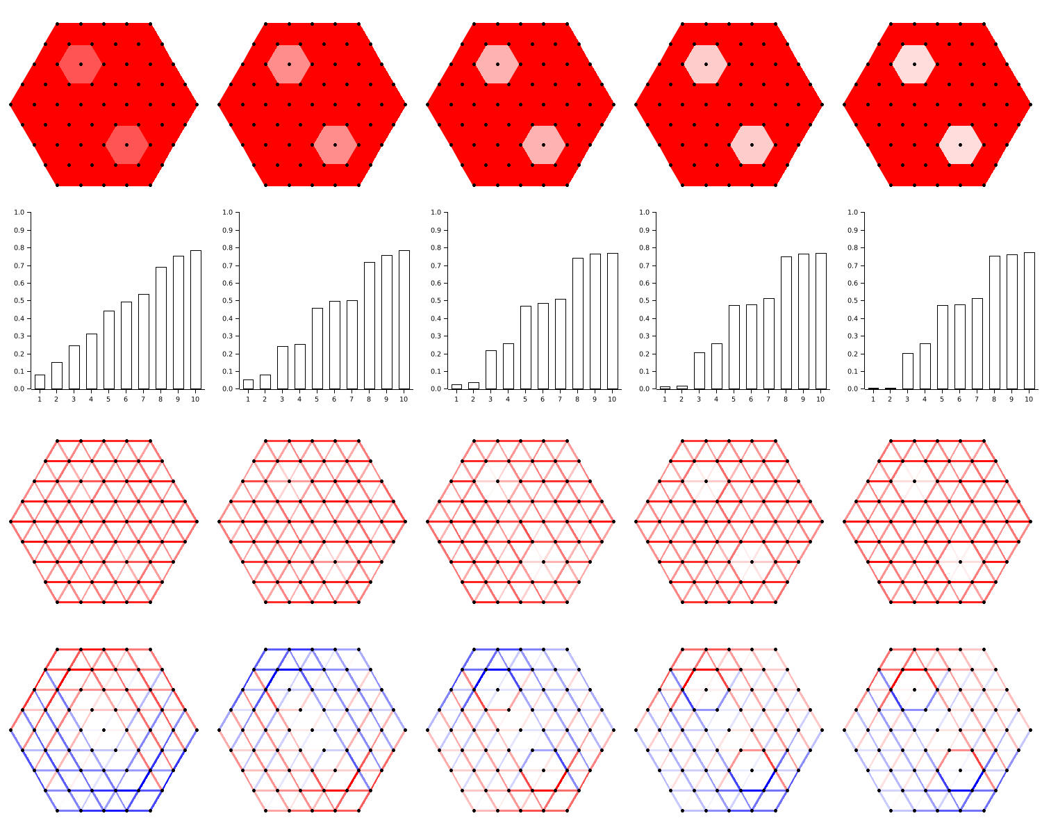
Figure 8 shows the computational results for a sequence of weighted simplicial complexes, where the weights of some of simplices gradually decrease. Each of the five simplicial complexes have no combinatorial holes defined on it, but the two smallest eigenvalues are getting smaller and smaller as the two “almost holes” get significant.
4.1 Dynamic Coverage Repair of Sensor Network
Simplicial complexes are proved to be useful in studying coverage problems of the sensor network. Given sensors in and , the simplicial complex defined by
is called a Vietoris-Rips complex. One of the initial results that successfully used simplicial complexes in the coverage problem of sensor networks was by Silva et al. [5], which showed that whether or not the a region is covered by a sensor network is sufficient to perform a test on the algebraic image of its boundary in the simplicial chain complex. Using the Čech complex, a subcomplex of Vietoris-Rips complex, Derenick et al. [4] gave a distributed motion-planning algorithm for mobile robot team that can collapse the homology. They used a combinatorial method to detect the precise location of the holes and used it to compute the motion plans.
In this section, we present a more continuous, parameter-free coverage repair algorithm using the weighted combinatorial Laplacian. Since the weighted Laplacian can measure the "almost holes", there does not have to be combinatorially well-defined holes in the simplicial complex. Hence we can take our simplicial complex to be just a contractible complex (a hole-free complex), and thus, as opposed to the case of using Vietoris-Rips complex (or Čech complex), the algorithm does not depend on the particular choice of . Another advantage of using weighted Laplacian is the fact that the extremal eigenvalues are naturally piece-wise smooth functions of weights, and this gives an obvious candidate for an algorithm, that is, the gradient descent of the extremal eigenvalues with respect to the weights. If we define the weights to be again smooth functions of positions of the mobile robots in the plane, then we have a piece-wise smooth function that measures the significance of holes with respect to the positions of sensors.
Let us now be more specific. Given a set of points embedded in the Euclidean plane , we construct a 2-dimensional contractible complex by the Delaunay triangulation, that is, the triangulation on such that the open disk bounded by the circumcircle of any triangle of does not contain any point in . In fact, the use of Delaunay triangulation (or its dual, the Voronoi partition) has been a natural choice for sensor coverage problems; for example, see [2], [11]. We let the weight of each edge be the inverse of the Euclidean length of it in and then let the weight of a 2-simplex be the product of the weights of its boundary, that is,
for each 2-simplex . Under the assumption that the weight of the edge is always greater than 1 (which is possible by scaling the embedding as necessary), this choice of weight satisfy the filtration condition introduced in Section 3, and thus the resulting weighted simplicial complex has all the properties shown in the section. We then compute the first weighted Laplacian operator , its eigenvector corresponding to the non-zero smallest eigenvalue , and the gradient of with respect to the embedding of . Note that we need to compute the gradient because . We can then update the embedding by the positive scalar multiple of , and therefore obtains the following algorithm:

Here, DelaunayTriangulation is the subroutine that computes the Delaunay triangulation based on the embedding of points in , and is the subroutine that computes the weighted Laplacian matrix. A computational result of the algorithm with 80 iterations is shown in Figure 9.

4.2 Creation of Holes in Sensor Networks for Caging
As an inverse approach to our method, we show that it is also possible to create holes in the sensor network. Let be the number of holes that we would like to create in the simplicial complex. Then it is possible to create -holes in the complex by performing the gradient descent on the th smallest non-zero eigenvalue. A result of this algorithm is shown in Figure 10.
4.3 Relative Chain Complex and its Application to Coverage Repair of Sensor Network in a Domain with Obstacles
It is often the case that the mobile robots need to explore a domain with obstacles. In this situation, however, the Algorithm 1 cannot be used because the Laplacian would not know whether the hole it sees is a hole in the coverage or an obstacle. To handle this issue, we let the Laplacian operator forget about the hole made by the obstacles so that it can make sure the hole it sees is the hole of the coverage. This leads us to the notion of a relative chain complex, and we further define the relative Laplacian operator.
Let be the chain complex, and let be a subcomplex of , that is, each is a vector subspace of , and implies . Then we define the relative chain complex to be the chain complex with the -chains and the induced boundary maps . Because we have not assumed anything beyond being a chain complex, this construction of the relative complex works for the weighted chain complex we have defined in the previous section.
Having these notions in mind, we come back to the coverage repair algorithm with obstacles. Let be the set of positions of the mobile robots distributed in the planar domain. Assume further that there are obstacles in the domain and that, for each , there is an obstacles , represented as a disjoint embedding of discs into . Then we can choose a sufficiently fine discretization of the boundary of as a 1-dimensional simplicial complex. Now let be the simplicial complex build by the Delaunay triangulation over the union of and the vertices of ’s, and let be the minimal subcomplex of containing all the 2-simplexes that intersects the interior of the obstacle . If the is a sufficiently fine discretization of the boundary of , then we can guarantee that . We can now recursively compute the relative chain complex , with the base case . Then the Laplacian over the resulting chain complex is the weighted Laplacian operator that forgets about the holes created by obstacles. We know that , because for each , the following part of the long exact sequence
yields that . Thus the smallest eigenvalue of is non-zero, and therefore we have obtained the following algorithm:
Here, VerticesOf() is the function that takes in a simplicial complex and spits out the set of vertices of , and is the repulsive gradient that tries to keep mobile robots away from the obstacles and is nonzero only near the boundary of . Comparing this algorithm with the Algorithm 1, the repulsive gradient might seem a little unnatural. However, it is necessary; otherwise, some mobile robots will try to get inside the obstacles because the relative Laplacian operator forgets the concrete geometry of the obstacles. A numerical result from this algorithm is presented in Figure 11.

Appendix A Proofs
Proof of Proposition 2.2.
-
(a)
We show only, because the other inclusion is trivial. Suppose that for some . Then we must have by the self-adjointness, hence . The proof of the other statement is similar.
-
(b)
We show only, because the other inclusion is trivial. If , then by the bilinearity of the inner product, we have
The sum of two non-negative numbers being zero implies all summands are zero, and it is the case here because the inner product of two identical vectors are non-negative. Hence we conclude that and .
-
(c)
This is the direct consequence of and
∎
Proof of Theorem 2.3.
For each , we have
∎
Proof of Proposition 3.1.
Recall that all the results about the combinatorial Laplacian stated in Section 2 applies to our weighted Laplacian as well, and from the Proposition 2.2(c) we can deduce that is equal to either or . Hence,
Hence it suffices to show for each . In the case of , this is trivial. If , the weighted boundary matrix has the concrete form
for . Therefore, by the filtration condition, we obtain
which completes the proof. ∎
Proof of 3.2.
Note that we have the following equation;
where are natural inclusion maps and are natural projection maps, for . We have that , since does not have any -simplex by assumption. Furthermore, the inclusion maps preserve the norm, hence
∎
Proof of Lemma 3.3.
Choose a total ordering of , then it will induce a total ordering on , for which we will denote . For , write for some (). By assumption, for . Consider the set . Now define a permutation on by
is well-defined because if and for some then by assumption, and it is clear that is a cyclic permutation of order , that is, for each . On the other hand, we have
Now notice that
where . is only a permutation of the basis elements, thus it preserves the norm. Furthermore, . Hence,
∎
Proof of Theorem 3.4.
Let , be as above. We have the Mayer-Vietoris sequence about the union , which is an exact sequence of the form
(See [9]). By assumption (2) and (3), we find a cycle in that is trivial in but is nontrivial in both and . Then let be the unit vector in obtained by applying the Gram-Schmidt process to with respect to the basis vectors of . We show that this vector is the desired vector.
Since is sum of the cycle and boundaries in , itself is a cycle in , which implies that . Furthermore, since is orthogonal to the image of under , we have . Hence, using lemma 3.2, we have
Now it suffices to show . By assumption (4), each basis element with has at most one cell such that . Thus, if where each is a basis element of , then for each with , there is a unique such that . Therefore,
| (by the assumption (1)) | ||||
| (by the assumption (5)) | ||||
| (by Lemma 3.3) | ||||
where the last inequality is by the fact that is a unit vector. ∎
Proof of 3.5.
For each union operation , choose as we have chosen in the proof of Theorem 3.4. Then forms an orthonormal basis of -dimensional vector space of , because ’s are pairwise disjoint and takes nonzero values only on . By assumption, we can deduce that , and by definition we have . Hence we can choose an orthogonal transformation such that for all . By the choice of , it is automatic that the equation (7) holds, that is a unit vector, and that is a cycle in . Now we can apply the same argument about in Theorem 3.4 to each to verify that (6) is satisfied. ∎
References
- \bibcommenthead
- Arnold et al. [2010] Arnold, D., Falk, R., Winther, R.: Finite element exterior calculus: from hodge theory to numerical stability. Bulletin of the American mathematical society 47(2), 281–354 (2010)
- Cortes et al. [2004] Cortes, J., Martinez, S., Karatas, T., Bullo, F.: Coverage control for mobile sensing networks. IEEE Transactions on Robotics and Automation 20(2), 243–255 (2004) https://doi.org/10.1109/TRA.2004.824698
- Cvetković and Simić [2010] Cvetković, D., Simić, S.K.: Towards a spectral theory of graphs based on the signless laplacian, ii. Linear Algebra and its Applications 432(9), 2257–2272 (2010) https://doi.org/10.1016/j.laa.2009.05.020 . Special Issue devoted to Selected Papers presented at the Workshop on Spectral Graph Theory with Applications on Computer Science, Combinatorial Optimization and Chemistry (Rio de Janeiro, 2008)
- Derenick et al. [2010] Derenick, J., Kumar, V., Jadbabaie, A.: Towards simplicial coverage repair for mobile robot teams. 2010 IEEE International Conference on Robotics and Automation, 5472–5477 (2010) https://doi.org/10.1109/ROBOT.2010.5509808
- de Silva V [2006] Silva V, G.R.: Coordinate-free coverage in sensor networks with controlled boundaries via homology. The International Journal of Robotics Research 25(12), 1205–1222 (2006) https://doi.org/10.1177/0278364906072252
- Fiedler [1973] Fiedler, M.: Algebraic connectivity of graphs. Czechoslovak Mathematical Journal 23, 298–305 (1973) https://doi.org/10.21136/CMJ.1973.101168
- Ghrist [2014] Ghrist, R.W.: Elementary Applied Topology vol. 1. Createspace Seattle, ??? (2014)
- Godsil et al. [2001] Godsil, C., Royle, C.D.G.G., Royle, G.F.: Algebraic Graph Theory. Graduate Texts in Mathematics. Springer, ??? (2001). https://books.google.com/books?id=gk60QgAACAAJ
- Hatcher [2002] Hatcher, A.: Algebraic Topology, p. 544. Cambridge University Press, Cambridge (2002)
- Newman et al. [2006] Newman, M.E., Barabasi, A.-L.E., Watts, D.J.: The Structure and Dynamics of Networks. Princeton university press, ??? (2006)
- Pimenta et al. [2008] Pimenta, L.C.A., Kumar, V., Mesquita, R.C., Pereira, G.A.S.: Sensing and coverage for a network of heterogeneous robots. In: 2008 47th IEEE Conference on Decision and Control, pp. 3947–3952 (2008). https://doi.org/10.1109/CDC.2008.4739194
- Zhang et al. [2021] Zhang, L., Sadler, B.M., Blum, R.S., Bhattacharya, S.: Inter-cluster transmission control using graph modal barriers. IEEE Transactions on Signal and Information Processing over Networks 7, 275–293 (2021) https://doi.org/10.1109/TSIPN.2021.3071219
- Zavlanos et al. [2008] Zavlanos, M.M., Tahbaz-Salehi, A., Jadbabaie, A., Pappas, G.J.: Distributed topology control of dynamic networks. In: 2008 American Control Conference, pp. 2660–2665 (2008). IEEE