Weak first-order phase transitions in the frustrated square lattice - classical Ising model
Abstract
The classical - Ising model on the square lattice is a minimal model of frustrated magnetism whose phase boundaries have remained under scrutiny for decades. Signs of first-order phase transitions have appeared in some studies, but strong evidence remains lacking. The current consensus, based upon the numerical data and theoretical arguments in [S. Jin et al., Phys. Rev. Lett. 108, 045702 (2012)], is that first-order phase transitions are ruled out in the region . We point out a loophole in the basis for this consensus, and we find strong evidence that the phase boundary is instead weak first-order at such that it asymptotically becomes second-order when . We also find strong evidence that the phase boundary is first-order in the region . We establish these results with adiabatic evolution of matrix product states directly in the thermodynamic limit, and with the theory of finite entanglement scaling. We also find suggestive evidence that when , the phase boundary becomes of an anomalous first-order type wherein the correlation length is very large in one of the coexisting phases but very small in the other.
I Introduction
The study of minimal models is well known to provide valuable fundamental insights. A seminal example is the understanding of thermal phase transitions gleaned from the classical Ising model on the square lattice with only nearest-neighbor interactions. Adding next-nearest-neighbor (i.e., diagonal) interactions to that model provides us with a minimal model of frustrated magnetism. Its Hamiltonian is given by
| (1) |
where and respectively denote nearest and next-nearest-neighbors, and . Frustration arises when : the nearest-neighbor and next-nearest-neighbor terms can not be simultaneously minimized on any minimal plaquette of the lattice (regardless of the sign of ). While the phases of this model are well understood, a complete understanding of the order of its phase boundaries has eluded decades of effort [1, 2, 3, 4, 5, 6, 7, 8, 9, 10, 11, 12, 13, 14, 15, 16, 17, 18, 19, 20, 21, 22, 23, 24, 25, 26, 27, 28, 29, 30, 31, 32, 33] (see Refs. 29, 30 for recent summaries).
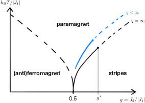
The phase diagram is illustrated in Fig. 1). The phase transition at occurs at zero temperature [30, 34]. The low temperature phase is either ferromagnetic () or antiferromagnetic () when , and stripe-ordered when , where . Both low temperature phases transition directly to a paramagnetic phase. Thus, this model provides an opportunity to study a phase transition between striped and paramagnetic phases.
Regarding , the phase boundary must go to Ising universality when , where the model becomes two decoupled copies of the nearest-neighbor square lattice Ising model. The current consensus, based on Refs. [23, 24, 25, 26], is that of second-order transitions at . The order of the transitions at remains uncertain; there is suggestive evidence that at least part of it is weak first-order [11, 12, 14, 17, 18, 19, 20, 24, 27, 30, 32], but also suggestive evidence that it is entirely second order [15, 22].
Regarding , the phase boundary must go to Ising universality when . A few studies find suggestive evidence for first-order transitions in a contiguous range of up to [30, 24, 27, 31, 33], but strong results are lacking.
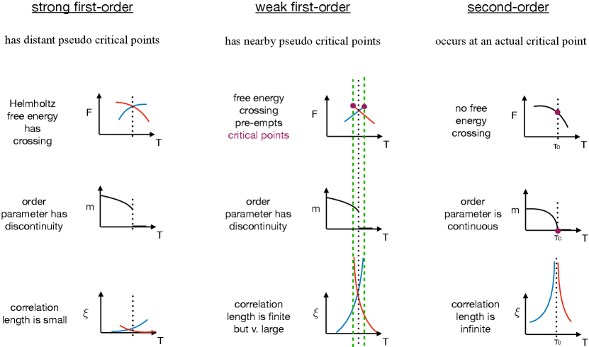
The difficulty in determining the order of the phase transitions in this model is essentially due to the difficulty in numerically distinguishing between weak first-order and second order phase transitions. We illuminate the salient features of weak first-order phase transitions that give rise to this difficulty via a comparison between strong and weak first-order phase transitions: Both strong and weak first-order phase transitions necessarily entail a discontinuity in the first derivative of the Helmholtz free energy and a discontinuity of the order parameter (see Fig. 2). Both also entail metastable branches of finite extent (terminating at spinodal points) in the phase diagram. As a spinodal point is approached along a metastable branch, the metastable state approaches criticality as if there were a critical point (termed a pseudo critical point [36, 37] 111This usage of “pseudo critical point” is different from the usage in Ref. [58]. or pseudospinodal point [39]) located beyond (or, in the mean-field limit, precisely at) the spinodal point [39]. Around a weak first-order phase transition, these pseudo critical points lie very close to the phase transition, which makes the coexistence region very small and imparts a large (but still finite) correlation length to the phase transition. Around a strong first-order phase transition, the pseudo critical points are far from the phase transition, and the correlation lengths are therefore small. For a weak first-order phase transition, the smallness of the coexistence region means that the hysteresis is difficult to resolve, and the large correlation lengths can make weak first-order phase transitions numerically appear as second-order phase transitions [40].
For the region in the present model, all existing results that show first-order signatures leave open the possibility that those first-order signatures are only numerical artifacts (due to, for example, finite cluster size), and all existing results that show second-order signatures leave open the possibility that those second-order signatures are in reality due to weak first-order phase transitions. For the region , the same is true for all results that appear prior to Ref. [23]. The authors of Ref. [23] (seemingly) make a breakthrough by combining numerical data with theoretical arguments instead of relying upon numerical data alone. Specifically, they (seemingly) rule out the possibility of first-order transitions at in the following way: because the present model has a theoretically known second-order phase transition at , they [23] assume that there is a line of second-order transitions that connects to it, and they combine numerical data with theoretical arguments to conclude that this line of second-order transitions in the region maps on to a phase boundary of the Ashkin-Teller model that exhibits continuously varying critical exponents. Subsequent numerics [24, 25, 26] confirm signatures of this “Ashkin-Teller criticality” at , hence the current consensus.
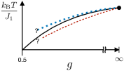
However, this consensus overlooks the fact that the theoretical arguments in Ref. [23] do not rule out an alternative possibility that is also consistent with the numerical data: a line of weak first-order phase transitions at that asymptotically turns into second-order transitions as . This is possible because a line of weak first-order phase transitions necessarily has a line of pseudo critical points on each side, and these three lines can asymptotically merge as ; see Fig. 3. The mapping onto the Ashkin-Teller model would then apply to one or both of the pseudo critical lines instead of the phase boundary itself. Since weak first-order phase transitions can numerically appear as second-order phase transitions [40], the results [24, 25, 26] indicating Ashkin-Teller criticality at do not contradict this scenario. When , the two pseudo critical lines in this scenario become a single critical point, whose central charge must be for consistency with the Ashkin-Teller criticality of one or both of the pseudo critical lines. The central charge is a measure of the number of local degrees of freedom, and thus the two central charges of the pseudo critical lines do not add together at because the number of degrees of freedom does not change when . This is consistent with the fact that at the model is two decoupled copies of the ordinary Ising model, each of which has central charge , and each of which also has only half the number of degrees of freedom of the full model.
Below we present strong evidence that this alternative scenario is the actual case. Further, we present strong evidence that the phase transitions in are also first-order. These results comprise strong evidence for first-order phase transitions in this model; the evidence is strong instead of only suggestive because we take care to show that it is highly unlikely that the first-order signatures that we find are mere numerical artifacts.
Additionally, from the discussion above and from Fig. 2 it seems plausible that there can be a first-order phase transition where the correlation length is very large in one phase but very small in the other; we find suggestive evidence that this is what occurs as in this model. Such a first-order phase transition can neither be categorized as a weak first-order phase transition nor as a strong first-order phase transition. We are not aware of any previous suggestions in the literature of such a scenario.
In Sec. II we explain the numerical method that we employ. In Sec. III we present numerical data that reveals the signatures of weak and anomalous first-order phase transitions. In Sec. IV we present further data and theoretical arguments to show that the first-order signatures are not numerical artifacts. In Sec. V we conclude with a discussion.
II Numerical Method
The class of computational methods designed around tensor networks [41, 42, 43, 44, 45, 46] is useful for studying both classical and quantum spin lattices; the following results from that field provide the basis for the numerical method of the present work: Ref. [47] demonstrates with a quantum 2D spin lattice that adiabatic evolution of 2D tensor networks is able to reveal ground state energy density level crossings and order parameter discontinuities directly in the thermodynamic limit. Ref. [48] demonstrates how to use a 1D tensor network, known as a matrix product state (MPS), to compute local observables directly in the thermodynamic limit of a classical 2D spin lattice. This MPS approach amounts to a power method wherein the row-to-row transfer operator of the partition function is repeatedly applied to the MPS until the MPS is sufficiently converged toward the dominant eigenvector of the transfer operator; direct access to the thermodynamic limit is provided by presuming translation invariance up to a chosen unit cell size and computing with only a single unit cell. The converged MPS may be interpreted as the groundstate wavefunction of a quantum 1D system that is dual to the classical 2D system [49, 50], and the correlations in the MPS may be interpreted as the bipartite entanglement in that wavefunction. The entanglement capacity of an MPS is limited by the size of its matrices, and this approach therefore suffers from finite-entanglement effects instead of finite-size effects.
We use the tensor network representation of the partition function for the present model that is given in the Appendix of Ref. [51]. We compute the Helmholtz free energy density and order parameter with an MPS method similar to that in Ref. [48].
The converged MPS gives ready access to the Schmidt decomposition of the one-dimensional wavefunction that it represents:
| (2) |
where () are states of the left (right) half of a bipartition of the system, are real scalars in descending order, , , and (known as the bond dimension) limits the entanglement capacity of the MPS and also determines the computational cost of its storage and manipulation. A single application of the transfer operator to the MPS results in an increase of the bond dimension to , after which the Schmidt decomposition must be truncated (and renormalized) to keep the first terms only; the sum is known as the truncation error.
The converged MPS also gives ready access to the correlation length [44]. While a more accurate method for computing the correlation length from the MPS exists [52], the simple method in Ref. [44] is sufficient for our goal here of arriving at only a qualitative understanding.
For each value of , we perform independent adiabatic evolutions with fixed values of using a two-site unit cell (represented by an MPS with two tensors, one for each physical site). For each adiabatic evolution in temperature at a given value of , we first converge a randomly initialized MPS with the transfer operator at the starting temperature, compute the physical quantities with the converged MPS, then use that converged MPS as the initial MPS for convergence at the subsequent temperature; the rest of the adiabatic evolution is completed by using the converged MPS at each temperature as the initial MPS for the subsequent temperature. The entanglement entropy, given by
| (3) |
depends on both the local and nonlocal correlations in the MPS, and we therefore consider the MPS converged at a given temperature when is converged to within a chosen tolerance (). Adiabatic evolutions in at fixed temperature are done in an analogous way. This method becomes numerically exact in the limit of vanishing increments of or , , and . We note that a similar adiabatic evolution method for probing phase boundaries with MPSs is used in Refs. [53, 54], the difference being that their approach uses a variational method instead of a power method to converge the MPSs.
III Weak and anomalous first-order signatures
The order parameter is defined by
| (4) | |||||
| (5) |
where () is the number of lattice sites in the () direction, and () are the coordinates of a spin. The stripe-ordered phase can have either and or and .
We check for Helmholtz free energy density crossings at but find none. This by itself does not rule out the possibility of extremely weak first-order transitions at ; we return to this in Sec. V.
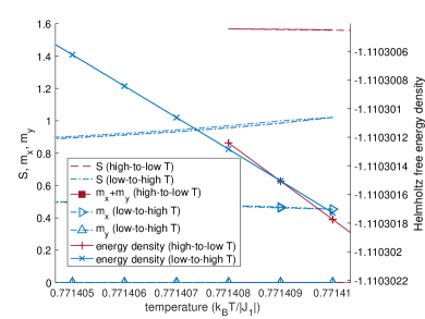
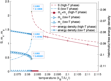
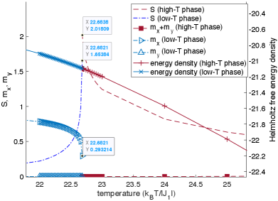
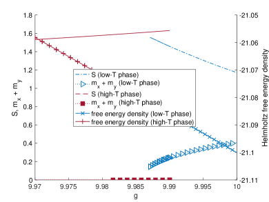
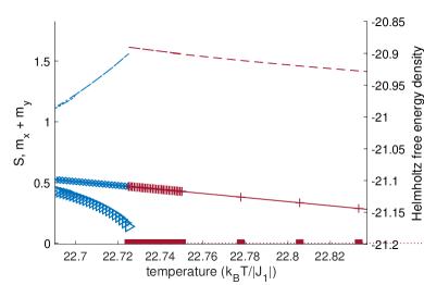
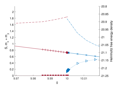
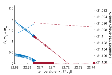
In Fig. 4) we illustrate the results of high-to-low and low-to-high adiabatic evolutions at with and e-6. The defining features of a first-order phase transition are apparent: a Helmholtz free energy density crossing occurs and the order parameter for the equilibrium state is discontinuous at the crossing.
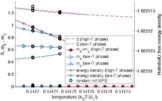
The apparent energy density crossing in Fig. 4) can not correspond to an energy density gap closing of a second-order transition for the following reasons: (1) As the gap-closing of a second-order transition is adiabatically approached from either side, the MPS must approach the same state and therefore the entanglement entropy () must approach the same value, whereas in Fig. 4) the two values of at the crossing differ greatly. (2) If the crossing is really a gap closing of a second-order transition, then the (quasi-)adiabatic evolution jumps from the ground state manifold to the excited state manifold as the crossing is traversed, which must result in a discontinuity in along either adiabatic path and a discontinuity in over the low-to-high path, but we find that both and are continuous over the energy density crossing along either adiabatic path. (3) A finite bond dimension imposes a finite correlation length [44] and therefore a finite gap, but there is no sign of a gap at the crossing point.
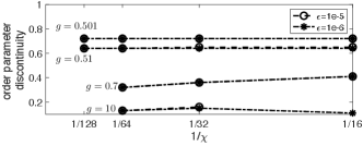
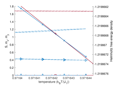
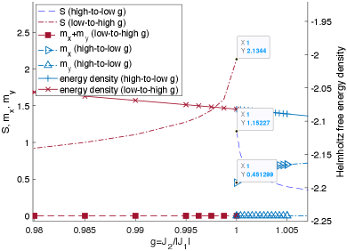
We perform adiabatic evolutions with different values of and at a series of . With increasing at fixed , the order parameter discontinuity (see Fig. 5) and the angle of incidence between the two free energy curves (see Fig. 6) both decrease. This is consistent with the requirement that the order parameter discontinuity and Helmholtz free energy crossing both disappear when . Though the discontinuity at is not very small, this is still compatible with the possibility that previous numerics mistakenly find second-order transitions there; the weak first-order phase transition of the classical square lattice 5-state Potts model has a large order parameter discontinuity (about 0.49) [35], yet appears as a second-order transition in certain finite-size numerics [40] 222A weak first-order transition may have a large order parameter discontinuity if the order parameter curve drops very steeply such that the energy crossing occurs at a large value of the order parameter yet is still very close to the pseudo critical point that lies at the zero point of the order parameter curve..
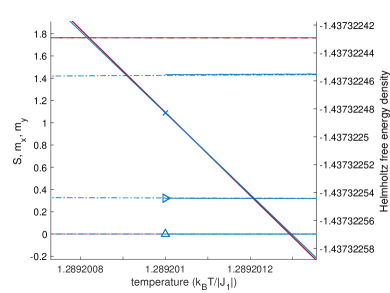
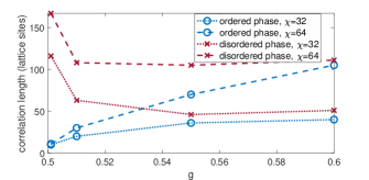
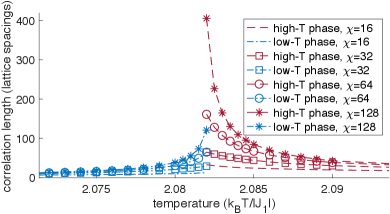
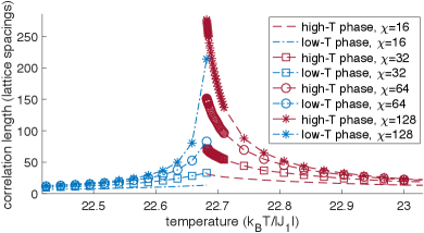
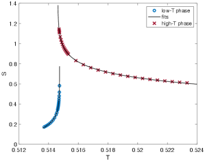
We also compute the correlation length in each phase near the phase boundary, as shown in Figs. (7), (8), and (9). We obtain the data in Fig. 9) with e-4. Converging to within this value of is sufficient for the correlation length data near the phase boundary because near criticality, [56], where is the central charge and is the correlation length; e-4 yields an error in of at most .
The large correlation lengths and their hysteresis that we find near the phase boundary are consistent with weak first-order transitions in the region , and are also consistent with the numerical detection of criticality in the region in Refs. [25, 26] because, as mentioned above, weak first-order phase transitions can numerically appear as second-order phase transitions. The hysteresis (assuming it is not a numerical artifact), however, is not consistent with actual second-order transitions. Interestingly, the data in Fig. 7) suggests that as , a first-order transition arises that is neither strong nor weak but part of both: the correlation length is very large in one phase but very small in the other. Further investigation of this is left for future work.

Thus, we find numerical evidence for first-order phase transitions in the region . This is at odds with the current consensus of second-order transitions in the region , but is consistent with the alternative possibility explained in Sec. I of first-order transitions in the region . However, our numerical evidence necessarily contains contributions from numerical imperfections, such as finite bond dimension. In the next section we show that such contributions are not responsible for the first-order signatures that we find, and thereby that our evidence for first-order phase transitions in the region is strong. We also explain why this leads to the conclusion that the first-order phase boundary only asymptotically becomes second-order as .
IV Consideration of numerical imperfections
IV.1 Imperfect adiabaticity
Here we address the possibility that the first-order signatures presented in Sec. III are mere artifacts due to imperfect adiabaticity. We note that on each adiabatic path we sweep the temperature back over the crossing after the extremal temperature is reached but we find only a negligible change. We perform additional checks at , , and : At we converge ten randomly initialized MPSs at each of two temperatures, one above and one below the crossing, and find good agreement with the adiabatic data (see Fig.4). At and this check is computationally prohibitive due to the small angle of incidence between the two energy curves 333We employ a power method, for which the rate of convergence to the equilibrium state is proportional to the energy gap., so we compare the results of adiabatic evolutions in (having fixed ) to the results of adiabatic evolutions in (having fixed ) such that both sets of evolutions meet at the same point in the phase diagram close to the phase boundary (either (, ) or (, )). In Appendix A we show that these complementary evolutions result in the same order parameter discontinuity and in the same values of at the point where they meet; this would be highly unlikely to occur if there were significant contributions from imperfect adiabaticity. We therefore conclude that the first-order signatures that we find at are not an artifact of imperfect adiabaticity.
IV.2 Adiabatic evolutions with iTEBD
Appendix B of Ref. [58] suggests that performing adiabatic evolutions with iTEBD itself can lead to the appearance of false metastabilities at second-order phase transitions, and that these metastabilities disappear if instead randomly initialized MPSs are used with iTEBD at each of the chosen points of the phase diagram. Our data from randomly initialized MPSs rules out this possibility at (see Fig. 4). Further, since such artifacts do not arise at the very strongly frustrated value of , it is unlikely that they arise at larger values of (which have weaker frustration) when the same values of and are used. Also, we note that the model at is only a perturbation of the model at , which makes it unlikely that adiabatic evolutions with iTEBD produce artifactual energy crossing metastabilities at without doing so at ; our adiabatic evolutions at and (not shown) do not produce metastable energy crossings. Finally, we note that though Appendix B of Ref. [58] presents data of hysteresis in the order parameter when adiabatically traversing the critical point of the quantum 1D Ising chain as evidence of artifactual metastability arising from adiabatic evolution with iTEBD, they do not show any metastable energy crossings, and their order parameter data is consistent with an alternative scenario: delayed spontaneous symmetry breaking when evolving from the disordered phase into the ordered phase. We therefore conclude that the first-order signatures that we find at are not due to the numerical imperfections that are specific to adiabatic evolutions with iTEBD.
IV.3 Finite bond dimension
Here we address the possibility that the first-order transition signatures that we find at with finite are numerical artifacts that would disappear when .
IV.3.1 Numerical evidence
In Appendix B we show that near criticality, assuming conformal invariance, the entanglement entropy takes the form
| (6) |
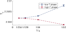
and that this allows us to compute, at given values of and , the value of via fitting. The value of computed in this manner will differ between the two sides of the phase transition at finite ; for a second-order phase transition the two values will converge toward the same value with increasing and decreasing , while for a first-order transition they will converge toward different values corresponding to the pseudo critical points.
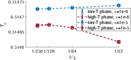
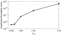
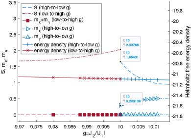
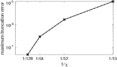
In Fig. 10 we show that the free energy density metastabilities that arise with adiabatic evolutions at do not change their location when is increased from to . Further, we show in Fig. 11 that the fitted value of from the high- side and the fitted value of from the low- side converge to different values with increasing , which is inconsistent with a second-order phase transition. In Fig. 12 we show the corresponding truncation error (see Sec. II for definition); the negligible truncation error at larger makes it unlikely that the data in Figs. 10 and 11 would qualitatively change if was increased further. The data in Fig. 11 is also converged in . We take this as strong evidence that the phase boundary at remains first-order when .
IV.3.2 Theoretical arguments
With increasing , the pseudo critical points move closer together and it becomes untenable to assess the limit through a purely numerical approach. We therefore assess the limit at larger by combining numerical data with the theory of finite entanglement scaling [58, 59, 60, 61, 62, 63] (also known as the theory of finite correlation length scaling), which provides a means of determining what happens in the limit by using data computed with only moderate values of . For example, Ref. [63] demonstrates that the theory of finite entanglement scaling can be used with infinite projected entangled pair states (a type of two dimensional tensor network) to successfully determine properties of second-order phase transitions without resort to achieving convergence in the bond dimension. This is analogous to how the theory of finite size scaling provides an understanding of the thermodynamic limit via computations with only modest system sizes.
We use the following results from the theory of finite entanglement scaling regarding how finite- effects in an MPS deform critical points: In a finite- MPS approximation of the ground state around a conformally invariant quantum 1D critical point, if is large enough to be within the finite- scaling limit (defined below), the divergence of the correlation length is replaced with a single finite peak [58]:
| (7) |
where is the value of the said peak and depends on the central charge () of the critical point [59, 60]:
| (8) |
Further, the location () of this peak evolves smoothly and monotonically as a function of such that it asymptotically goes to its true place () on the phase diagram when [58]:
| (9) |
where is the critical exponent from the standard correlation length scaling relation that arises near criticality. The finite- scaling limit is defined to be when . We note that the idea of a -dependent correlation length originally appeared in the context of the corner transfer matrix renormalization group in Ref. [64].
As mentioned, when the phase boundary of the present model necessarily becomes second-order. This remains true with a finite- MPS representation: in the limit , the model becomes two decoupled copies of the classical 2D Ising model, the classical 2D Ising model is in the same universality class as the quantum 1D transverse field Ising model [49, 65], and the phase transition of the latter model does not develop energy crossings and order parameter discontinuities when represented by a finite- MPS that is computed with iTEBD [58]. On the other hand, the data in Sec. III shows that when , the phase boundary in the region is first-order. Therefore, when there is a value of , denoted , at which the phase boundary switches between first-order and second-order (see Fig. 1). Then the picture established for regarding the pseudo critical lines and the phase boundary is the one in Fig. 3, except that the location of is only known to be somewhere in .
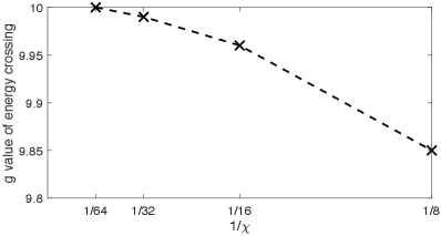
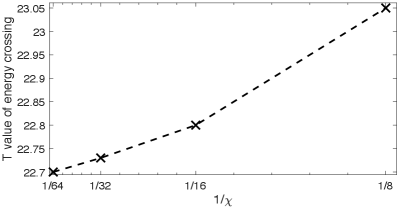
One way for the current consensus of to still remain true is for the entire phase boundary at to shift to lower values of as is increased from to . However, we can rule out this possibility because in Appendix C we show that, in accordance with Eq. (9), the phase boundary at monotonically shifts to larger values of when is increased above .
Then the only way left for the current consensus of second-order transitions at to remain true is if the two pseudo critical lines (see Fig. 3) fuse together as such that moves to or below . However, we can rule out this possibility as well since it results in a contradiction: If the pseudo critical lines that appear when fuse together with increasing such that when , then there is a line of true critical points at when that must split into two pseudo critical lines when is reduced from down to . But in Appendix D we explain that since falls within the finite- scaling limit at , Eq. (9) forbids critical points that occur at when to split into two pseudo critical lines as is reduced down to . We therefore have a lower bound of when .
Regarding the exact value of , because the model at is far from the region of strong frustration and is only a perturbation of the model at , it is unphysical that a switch of the phase boundary from first-order to second-order should occur at any finite value in . Therefore the only plausible scenario is that such that the first-order phase boundary only asymptotically becomes second-order as , as depicted in Fig. 3.
V Discussion
First-order phase transitions have long been suspected to occur in this model, yet strong evidence has remained absent. We addressed this in the following ways: We pointed out that the numerical data and theoretical arguments that form the basis for the current consensus of Ashkin-Teller criticality in the region leave open the possibility of an alternative scenario: weak first-order phase transitions at that asymptotically become second-order as . We presented data and theoretical arguments to provide strong evidence that this alternative scenario is the true one, and further that the phase boundary is also first-order in the region . In contrast to previous studies that presented only suggestive evidence for first-order transitions in this model, we established the first strong evidence by taking care to account for contributions from numerical imperfections. This was facilitated in part by the theory of finite entanglement scaling, which allowed us to make conclusions about the limit of infinite bond dimension () from data obtained with only modest . Additionally, we provided suggestive evidence that as , the first-order transitions become of a previously unobserved type that can be categorized as neither strong first-order nor weak first-order: the correlation length is very large in one coexisting phase and very small in the other.
The numerical correlation lengths at the phase boundary at are determined in part by the proximity of the pseudo critical lines to the phase boundary and in part by the value of . The locations of the pseudo critical lines shift with , as required by Eq. (9). Therefore, in order to confirm the anomalous first-order transitions at with the present approach of adiabatic evolutions of MPSs, values of in the region must be investigated showing convergence with increasing of both the correlation length data and the location of the pseudo critical lines. If the anomalous first-order transitions are confirmed in this model, it would be important to consider in which other models, both classical and quantum, they may also appear.
Regarding the pseudo critical lines themselves, while it is clear that they must merge with the phase boundary when , the following remains unclear: where the pseudo critical lines go when , which pseudo critical line exhibits the Ashkin-Teller criticality at , and what the criticality of either pseudo critical line is in the region . Recent results [32] indicate that at least one of the pseudo critical lines continues to have continuously varying critical exponents in the region . It may be possible to use the results in Refs. [58, 59, 60] to compute the critical exponents and central charge along the pseudo critical lines with MPSs.
We left open the possibility of an extremely weak first-order transition at . The fate of the pseudo critical lines at has a bearing on this: If the pseudo critical line for the disordered phase (i.e., the pseudo critical line at lower ) merges with the phase boundary as , it would give an infinite correlation length to the phase transition at from the high- side, and would thereby support the idea of a second-order transition at .
Finally, Ref. [66] showed good results for numerically detecting weak first-order phase transitions in other models with a different approach than the one used here. Future work may be able to use that approach as an independent check of the results that we have presented here.
Acknowledgements.
We acknowledge Anders Sandvik for drawing this problem to our attention and for discussions and feedback. We acknowledge Glen Evenbly for pointing out Ref. [47], for suggesting computation of pseudo critical point locations via fitting, and for technical help. We acknowledge Wangwei Lan for technical help and discussions. We also acknowledge discussions with Ying-Jer Kao, Ian McCulloch, Adam Iaizzi, André-Marie Tremblay, Thomas Baker, Ben Powell, Logan Wright, and Kai-Hsin Wu. This research was partly supported by the Australian Research Council Centre of Excellence for Engineered Quantum Systems (EQUS, CE170100009).References
- Nauenberg and Nienhuis [1974] M. Nauenberg and B. Nienhuis, Critical surface for square Ising spin lattice, Phys. Rev. Lett. 33, 944 (1974).
- Van Leeuwen [1975] J. Van Leeuwen, Singularities in the critical surface and universality for Ising-like spin systems, Phys. Rev. Lett. 34, 1056 (1975).
- Nightingale [1977] M. Nightingale, Non-universality for Ising-like spin systems, Phys. Lett. A 59, 486 (1977).
- Barber [1979] M. Barber, Non-universality in the Ising model with nearest and next-nearest neighbour interactions, J. Phys. A 12, 679 (1979).
- Oitmaa [1981] J. Oitmaa, The square-lattice Ising model with first and second neighbour interactions, J. Phys. A 14, 1159 (1981).
- Swendsen and Krinsky [1979] R. H. Swendsen and S. Krinsky, Monte Carlo renormalization group and Ising models with , Phys. Rev. Lett. 43, 177 (1979).
- Landau [1980] D. Landau, Phase transitions in the Ising square lattice with next-nearest-neighbor interactions, Phys. Rev. B 21, 1285 (1980).
- Binder and Landau [1980] K. Binder and D. Landau, Phase diagrams and critical behavior in Ising square lattices with nearest- and next-nearest-neighbor interactions, Phys. Rev. B 21, 1941 (1980).
- Landau and Binder [1985] D. Landau and K. Binder, Phase diagrams and critical behavior of Ising square lattices with nearest-, next-nearest-, and third-nearest-neighbor couplings, Phys. Rev. B 31, 5946 (1985).
- Aguilera-Granja and Morán-López [1993] F. Aguilera-Granja and J. Morán-López, Specific heat and the phase diagram of the Ising square lattice with nearest- and next-nearest interactions, J. Phys. Condens. Matter 5, A195 (1993).
- Morán-López et al. [1993] J. Morán-López, F. Aguilera-Granja, and J. M. Sanchez, First-order phase transitions in the Ising square lattice with first- and second-neighbor interactions, Phys. Rev. B 48, 3519 (1993).
- Morán-López et al. [1994] J. Morán-López, F. Aguilera-Granja, and J. M. Sanchez, Phase transitions in Ising square antiferromagnets with first- and second-neighbour interactions, J. Phys. Condens. Matter 6, 9759 (1994).
- Buzano and Pretti [1997] C. Buzano and M. Pretti, Cluster variation approach to the Ising square lattice with two-and four-spin interactions, Phys. Rev. B 56, 636 (1997).
- Lopez-Sandoval et al. [1999] E. Lopez-Sandoval, J. Moran-Lopez, and F. Aguilera-Granja, Cluster variation method and Monte Carlo simulations in Ising square antiferromagnets, Solid State Commun. 112, 437 (1999).
- Malakis et al. [2006] A. Malakis, P. Kalozoumis, and N. Tyraskis, Monte Carlo studies of the square Ising model with next-nearest-neighbor interactions, Eur. Phys. J. B 50, 63 (2006).
- Monroe and Kim [2007] J. L. Monroe and S.-Y. Kim, Phase diagram and critical exponent for the nearest-neighbor and next-nearest-neighbor interaction Ising model, Phys. Rev. E 76, 021123 (2007).
- dos Anjos et al. [2008] R. A. dos Anjos, J. R. Viana, and J. R. de Sousa, Phase diagram of the Ising antiferromagnet with nearest-neighbor and next-nearest-neighbor interactions on a square lattice, Phys. Lett. A 372, 1180 (2008).
- Kalz et al. [2008] A. Kalz, A. Honecker, S. Fuchs, and T. Pruschke, Phase diagram of the Ising square lattice with competing interactions, Eur. Phys. J. B 65, 533 (2008).
- Kalz et al. [2009] A. Kalz, A. Honecker, S. Fuchs, and T. Pruschke, Monte Carlo studies of the Ising square lattice with competing interactions, in J. Phys.: Conf. Ser., Vol. 145 (IOP Publishing, 2009) p. 012051.
- Kalz et al. [2011] A. Kalz, A. Honecker, and M. Moliner, Analysis of the phase transition for the Ising model on the frustrated square lattice, Phys. Rev. B 84, 174407 (2011).
- Murtazaev et al. [2011] A. Murtazaev, M. Ramazanov, and M. Badiev, Critical properties of an antiferromagnetic Ising model on a square lattice with interactions of the next-to-nearest neighbors, Low Temp. Phys. 37, 1001 (2011).
- Murtazaev et al. [2013] A. Murtazaev, M. Ramazanov, F. Kassan-Ogly, and M. Badiev, Phase transitions in the antiferromagnetic Ising model on a square lattice with next-nearest-neighbor interactions, J. Exp. Theor. Phys. 117, 1091 (2013).
- Jin et al. [2012] S. Jin, A. Sen, and A. W. Sandvik, Ashkin-Teller criticality and pseudo-first-order behavior in a frustrated Ising model on the square lattice, Phys. Rev. Lett. 108, 045702 (2012).
- Jin et al. [2013] S. Jin, A. Sen, W. Guo, and A. W. Sandvik, Phase transitions in the frustrated Ising model on the square lattice, Phys. Rev. B 87, 144406 (2013).
- Kalz and Honecker [2012] A. Kalz and A. Honecker, Location of the Potts-critical end point in the frustrated Ising model on the square lattice, Phys. Rev. B 86, 134410 (2012).
- Murtazaev et al. [2015] A. Murtazaev, M. Ramazanov, and M. Badiev, Critical properties of the two-dimensional Ising model on a square lattice with competing interactions, Physica B 476, 1 (2015).
- Bobák et al. [2015] A. Bobák, T. Lučivjanskỳ, M. Borovskỳ, and M. Žukovič, Phase transitions in a frustrated Ising antiferromagnet on a square lattice, Phys. Rev. E 91, 032145 (2015).
- Ramazanov et al. [2016] M. Ramazanov, A. Murtazaev, and M. Magomedov, Thermodynamic, critical properties and phase transitions of the Ising model on a square lattice with competing interactions, Solid State Commun. 233, 35 (2016).
- Li and Yang [2021] H. Li and L.-P. Yang, Tensor network simulation for the frustrated - Ising model on the square lattice, Phys. Rev. E 104, 024118 (2021).
- Hu and Charbonneau [2021] Y. Hu and P. Charbonneau, Numerical transfer matrix study of frustrated next-nearest-neighbor Ising models on square lattices, Phys. Rev. B 104, 144429 (2021).
- Abalmasov and Vugmeister [2023] V. Abalmasov and B. Vugmeister, Metastable states in the - Ising model, Phys. Rev. E 107, 034124 (2023).
- Yoshiyama and Hukushima [2023] K. Yoshiyama and K. Hukushima, Higher-order tensor renormalization group study of the - ising model on a square lattice, Physical Review E 108, 054124 (2023).
- Abalmasov [2023] V. Abalmasov, Free energy and metastable states in the square-lattice - Ising model, arXiv preprint arXiv:2310.20385 (2023).
- Lee et al. [2024] J. H. Lee, S.-Y. Kim, and J. M. Kim, Frustrated ising model with competing interactions on a square lattice, Physical Review B 109, 064422 (2024).
- Iglói and Carlon [1999] F. Iglói and E. Carlon, Boundary and bulk phase transitions in the two-dimensional Q-state Potts model (), Phys. Rev. B 59, 3783 (1999).
- Fernández et al. [1992] L. Fernández, J. Ruiz-Lorenzo, M. Lombardo, and A. Tarancón, Weak first order transitions. The two-dimensional Potts model, Phys. Lett. B 277, 485 (1992).
- Schülke and Zheng [2000] L. Schülke and B. Zheng, Dynamic approach to weak first-order phase transitions, Phys. Rev. E 62, 7482 (2000).
- Note [1] This usage of “pseudo critical point” is different from the usage in Ref. [58].
- Binder [1987] K. Binder, Theory of first-order phase transitions, Rep. Prog. Phys. 50, 783 (1987).
- Iino et al. [2019] S. Iino, S. Morita, N. Kawashima, and A. W. Sandvik, Detecting signals of weakly first-order phase transitions in two-dimensional Potts models, J. Phys. Soc. Jpn. 88, 034006 (2019).
- Verstraete et al. [2008] F. Verstraete, V. Murg, and J. I. Cirac, Matrix product states, projected entangled pair states, and variational renormalization group methods for quantum spin systems, Advances in physics 57, 143 (2008).
- Cirac and Verstraete [2009] J. I. Cirac and F. Verstraete, Renormalization and tensor product states in spin chains and lattices, J. Phys. A Math. Theor. 42, 504004 (2009).
- Eisert [2013] J. Eisert, Entanglement and tensor network states, in Emergent Phenomena in Correlated Matter, edited by E. Pavarini, E. Koch, and U. Schollwöck (Forschungszentrum Jülich, Jülich, 2013).
- Orús [2014] R. Orús, A practical introduction to tensor networks: Matrix product states and projected entangled pair states, Ann. Phys. (N.Y.) 349, 117 (2014).
- Bridgeman and Chubb [2017] J. C. Bridgeman and C. T. Chubb, Hand-waving and interpretive dance: an introductory course on tensor networks, J. Phys. A Math. Theor. 50, 223001 (2017).
- Orús [2019] R. Orús, Tensor networks for complex quantum systems, Nat. Rev. Phys 1, 538 (2019).
- Orús et al. [2009] R. Orús, A. C. Doherty, and G. Vidal, First order phase transition in the anisotropic quantum orbital compass model, Phys. Rev. Lett. 102, 077203 (2009).
- Orus and Vidal [2008] R. Orus and G. Vidal, Infinite time-evolving block decimation algorithm beyond unitary evolution, Phys. Rev. B 78, 155117 (2008).
- Suzuki [1976] M. Suzuki, Relationship between d-Dimensional Quantal Spin Systems and (d+ 1)-Dimensional Ising Systems: Equivalence, Critical Exponents and Systematic Approximants of the Partition Function and Spin Correlations, Prog. Theor. Phys. 56, 1454 (1976).
- Zauner et al. [2015] V. Zauner, D. Draxler, L. Vanderstraeten, M. Degroote, J. Haegeman, M. M. Rams, V. Stojevic, N. Schuch, and F. Verstraete, Transfer matrices and excitations with matrix product states, New J. Phys. 17, 053002 (2015).
- Gangat and Kao [2019] A. A. Gangat and Y.-J. Kao, Phase boundary location with information-theoretic entropy in tensor renormalization group flows, Phys. Rev. B 100, 094430 (2019).
- Rams et al. [2018] M. M. Rams, P. Czarnik, and L. Cincio, Precise extrapolation of the correlation function asymptotics in uniform tensor network states with application to the Bose-Hubbard and XXZ models, Phys. Rev. X 8, 041033 (2018).
- Roberts et al. [2019] B. Roberts, S. Jiang, and O. I. Motrunich, Deconfined quantum critical point in one dimension, Phys. Rev. B 99, 165143 (2019).
- Roberts et al. [2021] B. Roberts, S. Jiang, and O. I. Motrunich, One-dimensional model for deconfined criticality with Z3 Z3 symmetry, Phys. Rev. B 103, 155143 (2021).
- Note [2] A weak first-order transition may have a large order parameter discontinuity if the order parameter curve drops very steeply such that the energy crossing occurs at a large value of the order parameter yet is still very close to the pseudo critical point that lies at the zero point of the order parameter curve.
- Calabrese and Cardy [2006] P. Calabrese and J. Cardy, Entanglement entropy and quantum field theory: a non-technical introduction, Int. J. Quantum Inf. 4, 429 (2006).
- Note [3] We employ a power method, for which the rate of convergence to the equilibrium state is proportional to the energy gap.
- Tagliacozzo et al. [2008] L. Tagliacozzo, T. R. de Oliveira, S. Iblisdir, and J. Latorre, Scaling of entanglement support for matrix product states, Phys. Rev. B 78, 024410 (2008).
- Pollmann et al. [2009] F. Pollmann, S. Mukerjee, A. M. Turner, and J. E. Moore, Theory of finite-entanglement scaling at one-dimensional quantum critical points, Phys. Rev. Lett. 102, 255701 (2009).
- Pirvu et al. [2012] B. Pirvu, G. Vidal, F. Verstraete, and L. Tagliacozzo, Matrix product states for critical spin chains: Finite-size versus finite-entanglement scaling, Phys. Rev. B 86, 075117 (2012).
- Ueda et al. [2014] H. Ueda, K. Okunishi, and T. Nishino, Doubling of entanglement spectrum in tensor renormalization group, Phys. Rev. B 89, 075116 (2014).
- Corboz et al. [2018] P. Corboz, P. Czarnik, G. Kapteijns, and L. Tagliacozzo, Finite correlation length scaling with infinite projected entangled-pair states, Phys. Rev. X 8, 031031 (2018).
- Czarnik and Corboz [2019] P. Czarnik and P. Corboz, Finite correlation length scaling with infinite projected entangled pair states at finite temperature, Phys. Rev. B 99, 245107 (2019).
- Nishino et al. [1996] T. Nishino, K. Okunishi, and M. Kikuchi, Numerical renormalization group at criticality, Phys. Lett. A 213, 69 (1996).
- Gang and Xiang-Rong [2006] X. Gang and W. Xiang-Rong, A direct calculation of critical exponents of two-dimensional anisotropic Ising model, Commun. Theor. Phys. 45, 932 (2006).
- D’Emidio et al. [2023] J. D’Emidio, A. Eberharter, and A. Läuchli, Diagnosing weakly first-order phase transitions by coupling to order parameters, SciPost Phys. 15, 061 (2023).
- Léonard and Delamotte [2015] F. Léonard and B. Delamotte, Critical exponents can be different on the two sides of a transition: A generic mechanism, Phys. Rev. Lett. 115, 200601 (2015).
- Kramers and Wannier [1941] H. A. Kramers and G. H. Wannier, Statistics of the two-dimensional ferromagnet. Part I, Physical Review 60, 252 (1941).
- Pfeuty [1970] P. Pfeuty, The one-dimensional Ising model with a transverse field, Ann. Phys. 57, 79 (1970).
- Sachdev [2011] S. Sachdev, Quantum Phase Transitions (Cambridge University Press, Cambridge, 2011).
Appendix A: hysteresis data demonstrating negligible contributions from imperfect adiabaticity
V.1
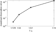
We use adiabatic evolutions in at and adiabatic evolutions in at to observe hysteresis in (see Fig. 13). These evolutions all meet at the same point (, ) in the phase diagram. The evolutions in the low- phase show agreement at that point, and the evolutions in the high- phase also show agreement at that point. Since the evolutions in and the evolutions in are very distinct paths in the phase diagram, the errors that they accrue due to imperfect adiabaticity have very different origins. Thus, the agreement at the point of intersection of the evolutions would be highly unlikely if the errors due to imperfect adiabaticity were appreciable. We can therefore rule out the possibility that the hysteresis is merely an artifact of imperfect adiabaticity. For completeness, in Fig. 14 we show truncation error data from these adiabatic evolutions.
V.2
Appendix B: pseudo critical point location via entanglement entropy fitting
As mentioned in Sec. II, the converged MPS at a given point in the phase diagram of the classical 2D system is an approximate representation of the ground state of the quantum 1D system that is dual to the classical 2D system at that point in the phase diagram. For an infinite quantum 1D system near a conformally invariant critical point, Ref. [56] shows that the half chain entanglement entropy is given by
| (10) |
where is the central charge and is the correlation length of the quantum 1D system. Because of the duality, is the same between the quantum 1D system and its dual classical 2D system. Near criticality we also have and , where is the correlation length of the classical 2D system, and are small parameters, and the critical exponent is the same in both systems due to the duality. More precisely, , where is the temperature of the critical point, and the duality tells us that is a differentiable function of . Using a Taylor expansion around we can write , where is a constant. Noting that at the critical point (i.e., where ), we find . Close to the critical point we can therefore write
| (11) |
Since the half-chain entanglement entropy can be computed efficiently from the converged MPS, we may fit Eq. (11) to the numerical data obtained by adiabatically approaching the phase boundary from both high and low temperature at fixed values of . Fig. 16 shows an example. For a continuous phase transition, both and must be the same between the high- and low-temperature sides of the phase transition (though an exception can occur in anisotropic models, where it is possible that can be different between the two sides [67]). For a weak first-order phase transition, lies at the pseudo critical points and must therefore be different between the high- and low-temperature sides of the transition (see Fig. 2). It is also possible for to be different between the two sides of a weak first-order transition.
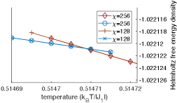
We use the known second-order phase transition at (, ) as a benchmark case for the fitting of and . We converge to within e- at each temperature step. We do not find good agreement between (not shown) as extracted from fits of Eq. (11) on the high- and low-temperature sides of the phase transition at , but we do find agreement of to high precision (see Table 1 and Fig. 17). We therefore only use fitted values of to draw conclusions at other values of (see Sec. IV).
| (low-) | (high-) | ||
|---|---|---|---|
| 32 | 2.269784411854 | 2.268866946007 | 9e-04 |
| 64 | 2.269285721313 | 2.269106864235 | 2e-04 |
| 128 | 2.269197257088 | 2.269167348571 | 3e-05 |
| 256 | 2.269181997444 | 2.269181205964 | 1e-06 |
Appendix C: monotonic shift of phase boundary at when
At the present system is two copies of the nearest neighbor classical Ising model on the square lattice, each of which has the Hamiltonian
| (12) |
where is a real scalar and the other variables are as defined in the Introduction, and whose critical temperature is given by [68]
| (13) |
where is Boltzmann’s constant.
If we write the nearest neighbor quantum 1D Ising model with a transverse magnetic field as
| (14) |
then it has a quantum phase transition at [69].
From Ref. [70] we know that there is a mapping between and such that
| (15) |
Thus, the value of in Eq. (14) fixes the value of in Eq. (12). Further, the mapping is such that both Hamiltonians become critical simultaneously, which fixes the critical value of at a value that we denote as :
| (16) |
As mentioned in Sec. IV, in a finite- MPS representation with sufficiently large , the quantum 1D critical point is shifted to a value so that:
| (17) |
Thus, combining Eqs. (13) and (17), we find that a monotonic shift in as a function of results in a monotonic shift in as a function of .
This establishes that the phase boundary at shifts smoothly and monotonically as a function of when is sufficiently large (i.e., within the finite- scaling limit). The same must be true for the entire phase boundary at , otherwise it would be unphysically crooked when .
The correlation length data in Fig. 9 shows that falls within the finite- scaling limit at . This is consistent with the fact that the model at is only a perturbation of the model at , and at the monotonic shift of the critical point with that is required by Eq. (9) is valid all the way down to [58]. It is also consistent with the numerical data in Figs. 18 and 19, which shows that the phase boundary around monotonically shifts, in agreement with Eq. (9), to larger values of and smaller values of as is increased from . Also, it is consistent with Eq. (7) in the following sense: At we have exactly [58], so we expect the prefactor in at to be close to unity since the model at is only a perturbation of the model at . If has a second-order phase transition, then previous results [23, 24, 25, 26] establish that it has central charge , which yields . Then at we easily satisfy when .
We therefore conclude that the entire phase boundary at monotonically shifts to larger values of as is increased above .
Appendix D: non-splitting of critical lines lines at when
Eq. (9) estalishes that conformally invariant quantum 1D critical points that appear within the finite- scaling limit (i.e., when is large enough so that ) can not split into two pseudo critical points as is varied within the finite- scaling limit. The results in Ref. [49] establish that the critical points of a given classical 2D spin lattice are equivalent to the critical points of some quantum 1D spin lattice. Therefore, conformally invariant critical points that appear in the present classical 2D model within the finite- scaling limit also can not split into two pseudo critical points as is varied within the finite- scaling limit.
If the present classical 2D model has a line of critical points at when , then Refs. [23, 24, 25, 26] establish that it must have conformal invariance with . Also, the correlation length data in Fig. 9 reveals at when , so lies within the scaling limit at . Therefore, Eq. (9) must apply to any line of critical points in the region when . This is consistent with the fact that is only a perturbation of the model at , the critical point of the model at maps, via the classical-quantum correspondence [49], on to the critical point of the quantum 1D Ising model, and Eq. (9) is valid for the latter all the way down to [58]. But Eq. (9) forbids a critical point from splitting into multiple pseudo critical points. It is therefore forbidden for a line of critical points that appear at when to split into two pseudo critical lines as is reduced down to .