Waveform Optimization with Multiple Performance Metrics for Broadband Joint Communication and Radar Sensing
Abstract
Joint communication and radar sensing (JCAS) integrates communication and radar/radio sensing into one system, sharing one transmitted signal. In this paper, we investigate JCAS waveform optimization underlying communication signals, where a base station detects radar targets and communicates with mobile users simultaneously. We first develop individual novel waveform optimization problems for communications and sensing, respectively. For communications, we propose a novel lower bound of sum rate by integrating multi-user interference and effective channel gain into one metric that simplifies the optimization of the sum rate. For radar sensing, we consider optimizing one of two metrics, the mutual information or the Cramér-Rao bound. Then, we formulate the JCAS problem by optimizing the communication metric under different constraints of the radar metric, and we obtain both closed-form solutions and iterative solutions to the non-convex JCAS optimization problem. Numerical results are provided and verify the proposed optimization solutions.
Index Terms:
Joint communication and radar sensing (JCAS), mobile networks, radar-communications, broadbandI Introduction
Sharing many hardware and signal processing modules and transmitting one single signal, joint communication and radar sensing (JCAS) systems have shown great potential in many applications. One main application is for the fifth-generation (5G) cellular networks or beyond [1, 2], where the transmitted signals are used for both providing communication services and sensing the surrounding environments. JCAS also brings a lot of interests in vehicular networks and self-driving [3, 4, 5], where signals used for communications between cars are also used for sensing the environment to detect objects and avoid collisions.
I-A Related Works
With most traditional hardware components replaced by digital processing modules, JCAS-enabled systems can reduce the number of connected devices and save the frequency resources [6, 7, 8]. To utilize the resources completely, most developed JCAS systems transmit single waveforms [9], except some works realizing JCAS functions via multiplexing technologies, such as time division multiplexing (TDM) [10], frequency division multiplexing (FDM) [11], or code division multiplexing (CDM) [12]. The resource utilization of single waveforms is highly efficient since the waveforms are shared by both communication and radar systems. Such waveforms can be developed from classical radar waveforms [13] or conventional communication waveforms [14].
Single waveform optimization has been reported in the literature. In [15], a multi-beam approach was proposed to flexibly generate JCAS sub-beams using analog antenna arrays. The optimization of the multi-beams was further investigated in [16]. This approach can adapt to varying channels but is suboptimal. In [17], the authors separated antenna arrays into two groups for realizing dual-function JCAS systems. The radar waveform falls into the nullspace of the downlink channel, such that the interference between radar signals and communication signals can be minimized. A multi-objective function was further applied to trade off the similarity between the generated waveform and the desired one in [18]. The multi-objective function in [18] is a weighted sum of two individual optimal waveforms. In [19], the authors maximized the radar signal-to-interference-plus-noise ratio (SINR) with a given specific capacity of communication channels. The work in [20, 21] further introduced a sub-sampling matrix for radar as an objective function of the optimization. It is noted that all these works studied waveform optimization in a narrowband scenario and ignored the frequency diversity.
When optimizing JCAS waveforms, different performance metrics for both communications and radar sensing can be used. The metrics for multiuser communication systems include multiuser interference (MUI) [18, 22] and effective channel gain (ECG) [23]. The MUI tolerance was analyzed for multi-input-multi-output orthogonal-frequency-division-multiplexing (MIMO-OFDM) JCAS systems in [22], using the interleaved signal model in [24]. The individual optimal communication waveform in [18] is also based on minimizing the MUI. However, simply minimizing MUI can cause the JCAS signals to fall into the nullspace of individual communication signals and result in a low SINR. To tackle this issue, the authors in [18] introduced an expected diagonal matrix that requires prior knowledge about the ECG.
As for radar sensing, typically considered performance metrics include mutual information (MI) [25, 26], Cramér-Rao bound (CRB) [9, 27], and minimum mean-squared error (MMSE) [28]. In [25], MI for an OFDM JCAS system was studied, and the power allocation on subcarriers was investigated by maximizing the weighted sum of the MI of radar and the MI of communication. In [26], the authors developed an MI measure that jointly optimizes the performance of radar and communication systems that overlap in the same frequency band. The CRB and MMSE are also commonly used metrics for waveform optimization. In [27], the authors derived the performance bounds in a single antenna system. In [28], the authors derived performance bounds for the radar estimation rate based on MMSE estimation bounds.
I-B Motivations and Contributions
Although the above-mentioned metrics have been individually studied for JCAS systems, no links between them have been identified so far. Some of those papers can be invalid when the number of sensing targets is not equal to that of the communication users. For communications, the SINR is the main concern, while most papers do not address the SINR directly and use some indirect metrics. For radar sensing, we note that different metrics can be used but there are no parallel comparisons. Based on the limitations of prior works, we aim to build a common method that can utilize different metrics for both communications and radar sensing.
This paper aims to develop waveform optimization algorithms for broadband JCAS systems and establish connections between different metrics of optimization. We consider a practical JCAS system of deployment. JCAS systems, particularly those underlying communication signals, confront the major challenge of full-duplex, that is, transmitting and receiving at the same time using the same frequency channel [29]. Solutions bypassing full-duplex requirements were discussed in [30, 31]. Here, we adopt a single receive antenna dedicated to radar sensing, which is a low-cost and practical solution at the moment.
The key idea is to optimize a developed novel lower bound of SINR for communications under different constraints of the radar metrics. By studying optimization with respect to these metrics together, for the first time, we disclose the important connections and relationships between these metrics in JCAS systems.
The main contributions of this paper are summarized as follows.
-
•
We derive multiple metrics, including MUI and ECG for communications, and MMSE, MI, and CRB for radar sensing, in a broadband JCAS system. In the adopted system, bypassing the full-duplex requirement, the base station (BS) uses one single receive antenna for collecting the signals reflected from targets.
-
•
We develop a novel lower bound of SINR as the communication metric, which contains both MUI and ECG. The developed lower bound simplifies the expression of SINR and makes it flexible for joint waveform optimization, involving both communication and radar metrics.
-
•
For radar sensing, we derive multiple metrics, including MMSE, MI, and CRB. We show the connections between optimizing these metrics.
-
•
We apply these multiple performance metrics and formulate two kinds of JCAS waveform optimization problems by minimizing the proposed communication metric under the constraint of the radar metric. We obtain the corresponding closed-form solutions under certain conditions. When the conditions are not satisfied, we propose iterative solutions based on Newton’s method.
Notations: denotes a vector, denotes a matrix, italic English letters like and lower-case Greek letters are a scalar. and represent determinant value, transpose, conjugate transpose, conjugate, and pseudo inverse, respectively. We use to denote a diagonal matrix with diagonal entries being the entries of . and represent the Frobenius norm and the th column of a matrix, respectively.
II System and Channel Models
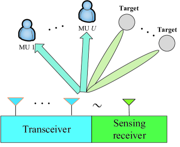
We consider an OFDM-based JCAS system supporting multiuser communications, as well as active downlink sensing. As shown in Fig. 1, the sensing is conducted at the BS, where an uniform linear array (ULA) is employed for simultaneous communications and radar sensing. Since the full-duplex technologies are not mature yet, we consider a low-cost alternative setup, where a single antenna, sufficiently separated from and synchronized with the transmit array, is used for solely collecting the reflected signals and detecting targets. Note that the sensing parameters can still be effectively estimated by using the received signal from the single-antenna receiver, except for the angle-of-arrivals (AoAs). The angle-of-departures (AoDs) can be obtained and serve a similar purpose as the AoAs.
The OFDM signal consists of subcarriers with the subcarrier interval being , where is the length of one OFDM symbol exclusive of the cyclic prefix (CP) of length . Letting denote a data symbol vector on subcarrier of the th time slot, we assume the data symbols are statistically independent, i.e., with being the transmit power. A digital precoder with the dimension of , , is applied to , such that . The precoded data symbol vector is written as
| (1) |
An inverse fast Fourier transform (IFFT) across the frequency band is then applied to the elements of from to and transforms signals into time domain. The time-domain signals are transmitted by the ULA.
The BS conducts downlink communications with multiple users (MUs) that are also potential targets. Each MU has a single receive antenna. It is noted that the system setup is equivalent to a multi-input-single-output (MISO) system. From [31] that adopts the same system setup, assembling from to would obtain highly accurate estimates of parameters. Hence, we assume that Doppler frequency approximately equals zero from to and make the system and channel model invariant to . Let us send a data block of length at the baseband of BS. The transmitted signals go through a beam-space multi-path channel. The received signal for each MU is sampled at the interval of and converted to the frequency domain using -point FFT’s after removing CP. The frequency-domain received signal block at the th MU is
| (2) |
where is the data block, is a complex AWGN vector with zero mean and covariance matrix of , and is a communication geometric channel, given by
| (3) |
where is the channel gain of the th path between BS and MU , is the equivalent AoD with being the actual AoD, is an normalized ULA array response vector, and is the time delay.
Meanwhile, the BS utilizes the single-antenna receiver to perform radar sensing. We assume that the transmitted signals from antennas impinge on targets with the time delays of . Let us denote the sensing channel as
| (4) |
where is the path loss coming from the th target, is the equivalent AoD with being the AoD, is the delay of the th target, , , , and is an vector with all entries being s. We assume that the entries of radar channel are independent and identically distributed (i.i.d.). In [31], a parameter sensing algorithm has been proposed to estimate the parameters using the adopted setup. Hence, in this paper, we assume that both radar and communication channels are known at the BS by using the estimation algorithms in [31], and focus on the waveform optimization.
The received frequency-domain signal at the BS for radar sensing is written as
| (5) |
where is a complex additive-white-Gaussian-noise (AWGN) vector with zero mean and covariance matrix of .
III Individual Performance Metrics
In this section, we will derive the performance metrics for communications and sensing individually. For communications, due to the non-convex nature of SINR, we propose and maximize a lower bound of SINR that is up to the MUI and the ECG of MUs. For radar sensing, we consider three different metrics, MMSE, MI, and CRB, and aim to disclose the links between these metrics.
III-A Metric for Communications
The sum rate or the SINR is the main concern for communications. However, the SINR has a non-convex form and can be difficult to optimize, especially when JCAS functions are required. In JCAS waveform optimization problems, both MUI and ECG have a dominant impact on the sum rate of communications. The MUI is on the denominator of SINR and can be expressed as
| (6) |
where , is the th column of , and denotes as the MUI of the th MU on the th subcarrier. Traditional optimization methods that mitigate MUI for communications only are not appropriate for JCAS problems, since only minimizing MUI can cause that the precoding vectors fall into the nullspace of , and result in a low ECG.
The ECG of MU-MISO systems is on the nominator of the SINR and can be written as
| (7) |
where denotes the ECG of the th MU on the th subcarrier. To make the following JCAS problems flexible and easy to solve, we develop a regulated bound of SINR as
| (8) |
where , , and is a weighting coefficient to balance between ECG and MUI.
The defined regulated bound, , can be seen as a lower bound of SINR when two conditions are satisfied. The first condition is . The second condition is . Generally, can be neglected at high SNRs. Hence, both conditions can be satisfied at high SNRs by letting , that is, we need to be zero.
Theorem 1.
is a lower bound of SINR when and , .
Proof.
The proof is shown in Appendix A. ∎
Theorem 1 unfolds that the defined metric, , is a lower bound of SINR as long as the SNR is sufficiently large and the scaled MUI is less than the ECG. We also note that, when the noise term is zero, the SINR is no smaller than . Hence, should be much larger than one at high SNRs to guarantee a high SINR.
By using to jointly optimize MUI and ECG, the individual waveform optimization problem for communications is formulated as
| (9) |
The minimization of is still a non-convex problem since is not semi-definite, but we note that has a much simpler expression than the SINR. Hence, When multiple metrics including both communication and radar are considered, can be a good substitute for the SINR. By performing the eigen-decomposition of , i.e., , we note that there exists one negative diagonal entry in . The optimal solution of should be the eigenvector with the corresponding eigenvalue being negative.
III-B MI and MMSE for Sensing
MI and MMSE are widely-used metrics in radar systems. Maximizing MI enables the maximization of information in the received signal, which contains the parameters of targets during its propagation. Minimizing MMSE is to obtain the parameters with the highest accuracy. With obtaining the accurate information about the targets, the parameters related to sensing can be extracted using various sensing algorithms.
The MI of the received OFDM symbols for sensing can be represented as
| (10) |
From (10), it is clear that maximizing MI is a convex problem and the optimal satisfies that , where is the left singular matrix of , that is, any satisfying is the optimal solution. The globally optimal should maximize the first singular value of . Hence, the optimal MI precoder has a rank of one. To make the precoder of dimension have only one rank, the optimal MI precoder is obtained as
| (11) |
where is an arbitrary matrix satisfying . Note that the size of the precoder is determined by the number of users instead of number of targets, since the number of targets can be varied from time to time.
The MMSE can be written as
| (12) |
where is the estimated radar channel. Referring to the derivations in [32], when is Gaussian distributed, we have the result of . Hence, the larger the transmit power is, the less the MMSE becomes. Due to the existence of noise, the MMSE reaches its minimum value that is larger than zero. Since MMSE is related to different sensing algorithms, we will use MI instead of MMSE as one radar metric for the following JCAS problem formulation.
III-C CRB for Sensing
CRB is a theoretical lower bound of MMSE. Note that CRB is not up to the sensing algorithms and generally cannot be achieved. In our adopted broadband MISO systems, we mainly consider the accuracy of estimates for delays, complex gains, and AoDs of the targets. The Doppler frequency is assumed to be zero in the training period. Note that the BS system setup is not a typical mono-static radar. We assume that it is an approximate mono-static radar for the convenience of deriving the CRB. We rewrite the received radar signal of (5) into the form of vector, i.e.,
| (13) |
where denotes the equivalent radar channel. Note that contains all parameters of interests, i.e., delays, complex gains, and AoDs, and contains the precoder to be determined. For convenience, we represent all parameters collectively using one common real-valued vector . It is noted that there are parameters in total. Hence, is a function with variables.
The CRB matrix, denoted as , contains all lower bounds of the estimates. The th entry of denotes the impact of the parameter on parameter . The total CRB can be expressed as the Frobenius norm of . The CRB matrix is the inverse matrix of Fish information matrix (FIM), i.e., . Referring to the derivations of [33] and using the so-called DOD/DOA Model defined in [33], we obtain our corresponding FIM as
| (18) |
where , and are given by Appendix B. The derivation can be referred to [33].
From Appendix B, we note that the CRB matrix depends on the covariance matrix, , only. Therefore, the CRB-based optimization problem is equivalent to optimizing . As we mentioned above, the total CRB equals the Frobenius norm of , which is equivalent to the sum of the singular values of . We aim to minimize the largest eigenvalue of the CRB matrix as in [34]. Minimizing the largest eigenvalue of the CRB matrix is equivalent to maximizing the smallest eigenvalue of the FIM. The waveform optimization under the eigen-optimization criterion can be directly formulated as a semi-definite-programming (SDP),
| (19) |
where is an auxiliary variable. However, the problem above is still difficult to address. We attempt to simplify the problem of (III-C). From Appendix B, we note that the norm of has an order of , which is significantly larger than that of other matrices in . Hence, we can approximately assume that equals , that is, only the accuracy of delays is counted.
Remark 1: Comparing MI and CRB, we note that they correspond to two types of optimization metrics. In the MI metric, the optimal waveform matrix can be obtained, while in the CRB metric, the optimal covariance waveform matrix can be obtained. For JCAS problem formulation, these two types of metrics also appear in many other metrics, such as channel capacity, desired semi-definite covariance matrix [18], and waveform similarity [35]. Hence, we will use these two types of optimal radar metrics and the proposed communication lower bound to formulate JCAS problems.
IV MI Constrained JCAS Waveform Optimization
In this section, we formulate optimization problems that jointly consider radar performance and communication performance. Note that in the section III, we have obtained one communication metric that contains both MUI and ECG, and obtained two radar metrics, one for MI and one for CRB. We will combine the communication metric with one of the radar metrics.
IV-A Closed-Form Solution
In this subsection, we constrain the MI of radar and simultaneously maximize the proposed lower bound of SINR, i.e., . Since the optimal MI is obtained via section III-B, we can define a threshold of MI, , that is smaller than the maximal MI. The MI-constrained JCAS optimization problem is formulated as
| (20) |
Note that minimizing the objective function above is not a convex problem, since in is not a semi-definite matrix. Hence, the problem above cannot be solved directly using convex-optimization toolboxes.
Since MI maximization is a convex problem, the range of that satisfies should be a convex set. Hence, we can directly transform the MI constraint set into another convex set. For the convenience of following proposed algorithm, we adopt the convex set that limits the Euclidean distance between the JCAS precoder and the optimal MI precoder, i.e.,
| (21) |
where is a threshold to constrain the Euclidean distance between the JCAS precoder and the optimal MI precoder. The transformed constraint is a complex sphere.
For the third constraint, we note that it has the same expression as the term in the objective function. As long as we can find an initial value of satisfying , we can use iterative solutions to make the objective function keep dropping.
For the fourth constraint, we note that the norm of can be an arbitrary value. Hence, as long as , we can make by suppressing the norm of . Hence, we omit the fourth constraint and transform the JCAS optimization problem of (IV-A) into
| (22) |
where . Note that all variables are subcarrier dependent. For notational simplicity, we omit the parameter in the following of this subsection.
We define the two constraint functions in (IV-A) as and , where is the th diagonal entry of .
Before optimizing , we note that in is still undetermined. It is clear to see that and are two complex spheres with the sphere center being and , respectively. The objective function of can be seen as a saddle surface with the saddle point being the original point. The gradient of is given by
| (23) |
We determine , such that the absolute value of gradient is maximized, i.e.,
| (24) |
By using Least Square method, is obtained as , where is a scaling factor, such that .
The objective function in (IV-A) is a quadratic optimization problem with convex constrained sets. Such problems can be iteratively solved by using Newton’s method [36]. Besides, we also obtain the closed-form solution, as demonstrated in Theorem 2 and Corollary 1.
Theorem 2.
The minimal value of in (IV-A) is achieved when is on the surface of the constrained sets.
Proof.
The proof is shown in Appendix C. ∎
According to Theorem 2, we obtain an important corollary that can directly obtain the closed-form solution of , which is illustrated as follows.
Corollary 1.
When there exist non-zero scaling factors, , such that or , the closed-formed solution of is obtained as .
Proof.
The proof is shown in Appendix D. ∎
However, the closed-form solution exists only when exists. In more general cases, we can obtain the following corollary.
Corollary 2.
The optimal point of is on the tangent plane of with being the minimal value.
Proof.
The proof is shown in Appendix E. ∎
IV-B Iterative Solution
Next, we propose an iterative algorithm based on Newton’s method [36], when the closed-form solution cannot be obtained. According to the proof of Theorem 2, we can make reach one surface of the constraints. When is on the surface of constraints, we aim to make the objective function be further decreased. Since there are two surfaces and only one will be reached, we consider two cases as follows.
IV-B1 Case 1: and
This case refers to the case when the surface of is first reached. The current iterative real-valued is denoted as and each column of is . We obtain two new columns moving in the directions of , with being defined in (46),
| (25) |
Note that neither nor satisfies that . Hence, we need to scale these columns onto the surface of , i.e.,
| (26) |
where , and are scaling coefficients, such that and , respectively.
The columns defined in (IV-B1) should make the objective function keep dropping. We select the one of which objective function is reduced, i.e.,
| (29) |
Updating the iteration index and repeat the same procedure. We terminate the iteration when stop dropping or when the other constraint is not satisfied, i.e.,
IV-B2 Case 2: and
In Case 2, we adopt the same strategy as Case 1. In this case, two temporary vectors are still given by (IV-B1). Then, we scale them onto the surface of , i.e.,
| (30) |
where are scaling coefficients, such that .
Likewise, we select the one of which objective function is less as in (29). Then we update the iteration index and repeat the same procedure. We terminate the iteration stop dropping or when the other constraint is not satisfied, i.e.,
IV-C Complexity Analysis
In this subsection, we analyze the computational complexity of Algorithm 1. The main computation tasks in Algorithm 1 include the eigen-decomposition of and the iterations. The complexity of the eigen-decomposition of can be given by . Since there are , the total complexity of eigen-decomposition is . The main steps in the iterations are Step 8 for Case 1 and Step 15 for Case 2, which both have a complexity of , due to the calculation of and . Hence, the complexity of the iterations is , where is the number of iterations. The overall complexity can be given by .
V CRB Constrained JCAS Waveform Optimization
In this section, we optimize the proposed communication metric, , with constraining the CRB of the radar. Intuitively, we would like to adopt the same strategy as in MI constrained problem, which controls the Euclidean distance between the precoder and the optimal individual radar precoder. Nevertheless, for individual CRB optimization, we obtain the optimal covariance matrix, denoted as , instead of the optimal . With a given , there are infinite solutions of . Not all the solutions are appropriate ones for the communication metric. Using the Euclidean distance between and would make the variables have an order of four and hence difficult to solve. Aiming to reduce the order of variables, we constrain the CRB by controlling
| (31) |
where is the threshold to control the CRB. This constraint has an order of two for the variables in .
Still, we omit the subcarrier in the following of this section. The JCAS optimization problem with the CRB constraint is formulated as
| (32) |
Similar to the MI constrained problem, the transformed CRB constrained problem can also be seen as a quadratic problem with convex constraints. Such problems can be solved using Newton’s method.
Referring to Corollary 1, the closed-form solution can be obtained when can reach the surfaces of or . When the closed-form solution does not exist, we propose an iterative algorithm as in Algorithm 1.
V-1 Case 3: and
In this case, two temporary vectors are still given by and of which expressions are given by (IV-B1). Then, we scale them onto the surface of . The new columns are given by
| (33) |
where are scaling coefficients, such that .
Likewise, we select the one of which objective function is less as in (29). Then we update the iteration index and repeat the same procedure. We terminate the iteration stop dropping or when the other constraint is not satisfied, i.e.,
V-2 Case 4: and
In Case 4, two temporary vectors are given by and . Then, we scale them onto the surface of , i.e.,
| (34) |
where are scaling coefficients, such that .
Likewise, we select the one of which objective function is less as in (29). Then, we update the iteration index and repeat the same procedure. We terminate the iteration when stop dropping or when the other constraint is not satisfied, i.e., The proposed CRB constrained optimization scheme is summarized in Algorithm 2. Note that from Case 1 to Case 4, all procedures are the same except the determination of the scaling coefficients and the terminating conditions.
VI Simulation Results
In this section, we provide simulation results to validate the proposed algorithms, following the system and channel models introduced in Section II. We simulate a JCAS system where a BS communicates with MUs each having paths and detects targets. The BS adopts a ULA as the transmit antennas and uses OFDM modulation to transmit a data symbol vector on each subcarrier. The number of subcarriers is . The AoDs for both MUs and targets are randomly distributed from to . The delay of each path is a random value ranging from 0 to ms. The period of one OFDM symbol is ms. For the parameter in the communication metric, we let . For parameters in the proposed algorithms, we let , , and .
We separate the simulation results into three subsections. In the following subsection VI-A, we show the achieved sum rates for communications and the achieved MI for radar sensing by using our proposed Algorithm 1. In subsection VI-B, we verify the sum rates for communications and the CRB for radar sensing by using the proposed Algorithm 2. For comparison, we compare our proposed algorithms with the bench-marking solutions, including the optimal individual solutions and the weighted sum JCAS solution that is proposed in [18]. In subsection VI-C, we aim to compare our proposed algorithms in parallel and figure out the impacts of using MI and CRB on optimizing JCAS waveforms.
VI-A MI Constrained JCAS
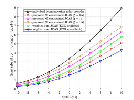
Fig. 2 shows how the sum rates vary with SNR using different JCAS solutions. For the individual communication precoder, the sum rate remains the highest. It is undoubted since the precoder is optimized solely for maximizing the sum rate. Regarding the JCAS solutions, we compare our proposed Algorithm 1 with the weighted-sum JCAS solution in [18]. The weighted-sum JCAS solution needs the prior knowledge about the ECG. We see that with ranging from 1 to 1.5, our proposed precoder achieves better performance than the weighted-sum JCAS solution. Moreover, our proposed algorithms do not need to know the value of ECG. When ECG is unavailable, we see that the sum rate of the weighted-sum JCAS solution drops substantially. Our proposed algorithm guarantees that the ratio of ECG to MUI is larger than . We can obtain the sum rate that is no smaller than at high SNRs. The MUI has a dominant impact on the sum rate when SNR is high, hence our proposed precoder can achieve better performance by further increasing .
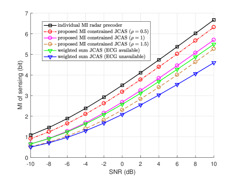
Fig. 3 unfolds the achieved MI of radar sensing versus SNR using different JCAS solutions. The system setup is the same as that in Fig. 2. The MI of individual MI radar precoder, i.e., , remains the highest. Our proposed Algorithm 1 achieves better MI than that of [18] when is no larger than 1. Without obtaining ECG, the MI of weight-sum JCAS solution declines greatly. By decreasing to zero, our proposed solution can achieve the MI of individual MI radar precoder. Together with Fig. 2, under the same power control, we notice that the sum rate is in proportion to while the MI is in inverse proportion to . To guarantee both good performances for communications and sensing, should be nearly 1.
VI-B CRB Constrained JCAS
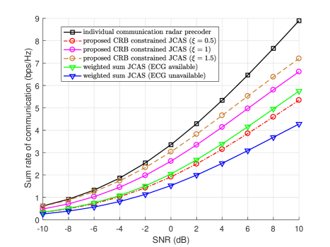
Fig. 4 depicts how the sum rates vary with SNR using Algorithm 2 and other solutions. Similar to Fig. 2, the sum rate of the individual communication precoder remains the highest. Regarding the JCAS solutions, we compare our proposed Algorithm 2 with the weighted-sum JCAS approach in [18]. We observe that, with ranging from 1 to 1.5, our proposed Algorithm 2 achieves better performance than the weighted-sum JCAS solution. Comparing with Fig. 2, We note that under the same control of , the achieved sum rate of Algorithm 2 is slightly better than that of Algorithm 1. We will discuss the gap later in Fig. 7.
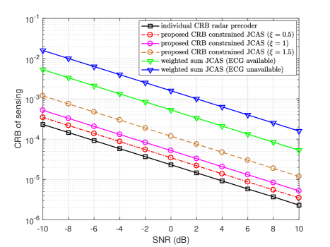
Fig. 5 illustrates the achieved CRB of radar sensing versus SNR using different JCAS solutions. The system setup is the same as that in Fig. 2. The individual CRB radar precoder achieves the lowest CRB among all solutions. Our proposed Algorithm 2 achieves lower CRB than that of [18] no matter the ECG is available or not. By decreasing to zero, our proposed solution can achieve the optimal lowest CRB. Together with Fig. 4, we can let range from to to guarantee both good performances for communication and sensing.
VI-C Comparisons of Proposed MI/CRB Constrained JCAS
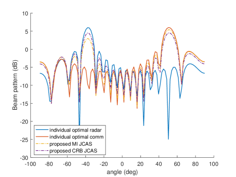
Fig. 6 illustrates an example of JCAS beam patterns with employing the proposed algorithms. To make the beam patterns clear to see, we only consider one MU and one target with only one path, i.e., , , and . For individual designs as illustrated in section III, we adopt the individual optimal MI radar precoder and the individual optimal communication precoder, respectively. We see that there is one main lobe located at around for the radar precoder, and one main lobe located at around for the communication precoder. For JCAS designs, both our proposed algorithms have two main lobes, matching with the locations of individual designs tightly. At the sidelobes, we see that our proposed JCAS solutions also have a good suppression, especially at the range of
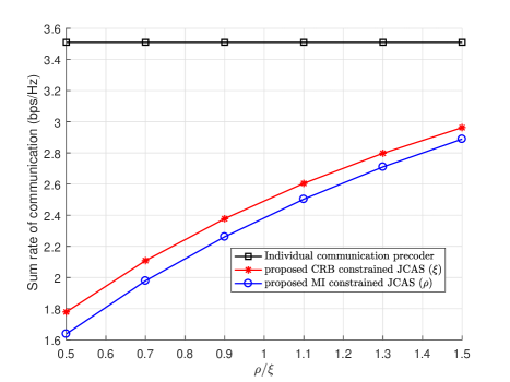
Next, we compare the proposed Algorithm 1 with Algorithm 2 under equal communication performance. This can unfold the impact of CRB and MI on the JCAS designs. To guarantee that Algorithm 1 and 2 achieve equal sum rates for communications, we simulate the sum rate versus threshold factors, (), as shown in Fig. 7. The system set up is the same as that in Fig. 2, except that the SNR is fixed at 0 dB. It is clear to see that, under the equal value of the threshold factors, Algorithm 2 achieves slightly better sum rates that Algorithm 1. When two proposed algorithms achieve equal sum rates, needs to be about 0.11 larger than . This result helps us to analyze the following two results.
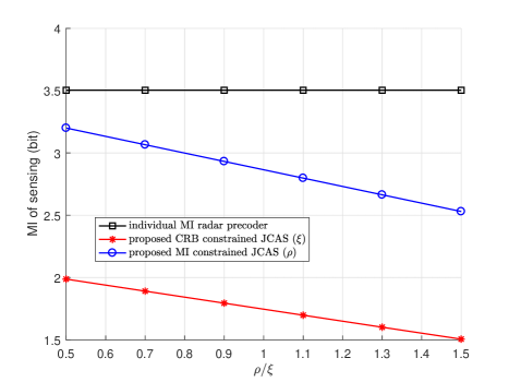
In Fig. 8, we aim to verify if Algorithm 2 can achieve effective MI. The system set up is the same as that in Fig. 7. Note that Algorithm 2 is designed for minimizing CRB. The MI of individual MI radar precoder remains the highest. Referring to the result in Fig. 7, we note that should be about 0.1 larger than to make the two proposed algorithms achieve an equal level of sum rates for communications. We see that the MI achieved by Algorithm 2 is significantly lower than that of Algorithm 1. With the same communication performances, the MI of Algorithm 2 is less that than the optimal solution by almost 2 bits. This could be explained by noting that the individual CRB radar precoder is close to the array response matrix, , instead of , which means that one column could be truncated by using the CRB precoder and results in the decline of MI for using the CRB constrained precoder.
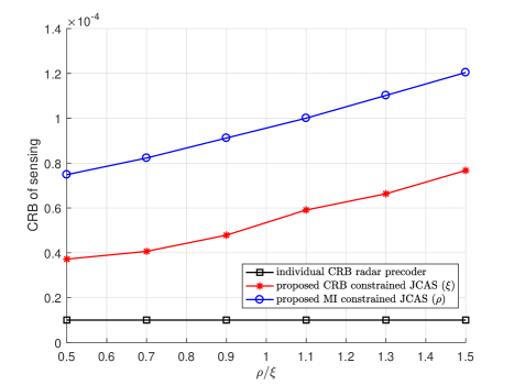
In Fig. 9, we aim to verify if Algorithm 1 can achieve effective CRB. The system set up is the same as that in Fig. 7. The CRB of individual CRB radar precoder remains the lowest. We observe that the CRB of Algorithm 1 is almost equal with that of Algorithm 2 and rises slightly with increasing . When is 0.1 larger than , the gap between the two algorithms is around . Even though the CRB of MI constrained algorithm is higher than that of the CRB constrained algorithm, the gap of can be neglected. Referring to Fig. 8, we see that the MI constrained optimization can achieve good performances on both MI and CRB. More importantly, the MI constrained optimization has a closed-form solution while the CRB constrained optimization has not. Hence, we can obtain a conclusion that maximizing MI is more efficient and simpler than minimizing CRB for JCAS optimization.
VII Conclusion
In this paper, we have proposed the JCAS waveform optimization algorithms that maximize the developed lower bound of communication sum rates under the constraint of either MI or CRB of radar. The adopted radar metrics correspond to two types of individual optimal radar matrices, i.e., precoding matrix and covariance matrix. The developed lower bound of communication rates balances between MUI and ECG, and serves as a good substitute for SINR. We have established the connections between different constrained optimizations and showed that MI constrained JCAS solution is more efficient and less complicated than the CRB constrained JCAS solution.
Appendix A Proof for Theorem 1
Given that and , we have . Then, we have
We note that the SINR is the sum of and is the sum of . Therefore, is a lower bound of SINR.
Appendix B Expression for FIM Subblocks
Referring to the derivation in [33], with including the precoding matrix, , the FIM subblocks are expressed as
| (35) |
where is Hadamard product,
| (36) |
and
| (37) |
Appendix C Proof for Theorem 2
Note that is a saddle face that is symmetric with respect to the origin point. We write in the real parts and imaginary parts, i.e.,
| (44) | |||
| (45) |
Supposed that there is an initial that satisfies both and , there exists a new column, , where is the th eigen vector of with being the rank of . The variable, , is small enough to make the new column inside the constraints. Note that is not a semi-definite matrix, the th eigen value is negative, denoted as , (when all eigen values are sorted in order). Hence, the new column, , satisfies
| (46) |
where means the value of with respect to . It is clear that the third term of (46) is negative. If the second term is also negative, we have . Hence, keeps dropping until is on the surface of the constraints. If the second term in (46) is positive, then we choose another column, i.e., , then the second term becomes negative. Therefore, the optimal is on the surface of the constraints.
Appendix D Proof for Corollary 1
According to Theorem 2, the optimal point of is on the surface of constraints. When is also on the surface of constraints, to further decrease the objective function from , the possible value of is given by , where is the th left eigenvector of . From the expression of , there is only one negative eigenvalue in , i.e., . Substituting into the objective function, we have
| (47) |
Hence, the possible value of cannot make the objective function keep dropping. Therefore, when is also on the surface of constraints, the closed-form solution of is solved as .
Appendix E Proof for Corollary 2
According to Theorem 2, the optimal point of is on the surface of constraints. For simplicity, we assume that the optimal is achieved when . In this case, the surface of and the surface of are tangent with each other. Otherwise, there will be a point of that satisfies and , which is contradictory with Theorem 2. Therefore, the optimal point of is on the tangent plane of with being the minimal value.
References
- [1] A. Abdelhadi and T. C. Clancy, “Network MIMO with partial cooperation between radar and cellular systems,” in 2016 International Conference on Computing, Networking and Communications (ICNC), Feb. 2016, pp. 1–5.
- [2] M. L. Rahman, P. Cui, J. A. Zhang, X. Huang, Y. J. Guo, and Z. Lu, “Joint communication and radar sensing in 5G mobile network by compressive sensing,” in 2019 19th International Symposium on Communications and Information Technologies (ISCIT), Sep. 2019, pp. 599–604.
- [3] P. Kumari, J. Choi, N. González-Prelcic, and R. W. Heath, “IEEE 802.11ad-based radar: An approach to joint vehicular communication-radar system,” IEEE Trans. Veh. Technol., vol. 67, no. 4, pp. 3012–3027, Apr. 2018.
- [4] R. C. Daniels, E. R. Yeh, and R. W. Heath, “Forward collision vehicular radar with IEEE 802.11: Feasibility demonstration through measurements,” IEEE Trans. Veh. Technol., vol. 67, no. 2, pp. 1404–1416, Feb. 2018.
- [5] S. H. Dokhanchi, M. R. B. Shankar, Y. A. Nijsure, T. Stifter, S. Sedighi, and B. Ottersten, “Joint automotive radar-communications waveform design,” in 2017 IEEE 28th Annual International Symposium on Personal, Indoor, and Mobile Radio Communications (PIMRC), Oct. 2017, pp. 1–7.
- [6] C. Sturm and W. Wiesbeck, “Waveform design and signal processing aspects for fusion of wireless communications and radar sensing,” Proc. IEEE, vol. 99, no. 7, pp. 1236–1259, Jul. 2011.
- [7] A. R. Chiriyath, B. Paul, and D. W. Bliss, “Radar-communications convergence: Coexistence, cooperation, and co-design,” IEEE Trans. on Cogn. Commun. Netw., vol. 3, no. 1, pp. 1–12, Mar. 2017.
- [8] L. Han and K. Wu, “Joint wireless communication and radar sensing systems - state of the art and future prospects,” IET Microwaves, Antennas Propagation, vol. 7, no. 11, pp. 876–885, Aug. 2013.
- [9] Y. Liu, G. Liao, Z. Yang, and J. Xu, “Multiobjective optimal waveform design for OFDM integrated radar and communication systems,” Signal Process., vol. 141, pp. 331–342, Jun. 2017.
- [10] L. Han and K. Wu, “Multifunctional transceiver for future intelligent transportation systems,” IEEE Trans. Microw. Theory Techn., vol. 59, no. 7, pp. 1879–1892, Jul. 2011.
- [11] A. K. Mishra and M. Inggs, “Fopen capabilities of commensal radars based on whitespace communication systems,” in 2014 IEEE International Conference on Electronics, Computing and Communication Technologies (CONECCT), 2014, pp. 1–5.
- [12] H. Takase and M. Shinriki, “A dual-use radar and communication system with complete complementary codes,” in 2014 15th International Radar Symposium (IRS), 2014, pp. 1–4.
- [13] S. D. Blunt, M. R. Cook, and J. Stiles, “Embedding information into radar emissions via waveform implementation,” in 2010 International waveform diversity and design conference, 2010, pp. 000 195–000 199.
- [14] Y. L. Sit and T. Zwick, “MIMO OFDM radar with communication and interference cancellation features,” in 2014 IEEE radar conference, 2014, pp. 0265–0268.
- [15] J. A. Zhang, X. Huang, Y. J. Guo, J. Yuan, and R. W. Heath, “Multibeam for joint communication and radar sensing using steerable analog antenna arrays,” IEEE Trans. Veh. Technol., vol. 68, no. 1, pp. 671–685, Jan. 2019.
- [16] Y. Luo, J. A. Zhang, X. Huang, W. Ni, and J. Pan, “Optimization and quantization of multibeam beamforming vector for joint communication and radio sensing,” IEEE Trans. Commun., vol. 67, no. 9, pp. 6468–6482, Sep. 2019.
- [17] F. Liu, C. Masouros, A. Li, H. Sun, and L. Hanzo, “MU-MIMO communications with MIMO radar: From co-existence to joint transmission,” IEEE Trans. Wireless Commun., vol. 17, no. 4, pp. 2755–2770, Apr. 2018.
- [18] F. Liu, L. Zhou, C. Masouros, A. Li, W. Luo, and A. Petropulu, “Toward dual-functional radar-communication systems: Optimal waveform design,” IEEE Trans. Signal Process., vol. 66, no. 16, pp. 4264–4279, Aug. 2018.
- [19] B. Li and A. Petropulu, “MIMO radar and communication spectrum sharing with clutter mitigation,” in 2016 IEEE Radar Conference (RadarConf), May 2016, pp. 1–6.
- [20] B. Li, A. P. Petropulu, and W. Trappe, “Optimum co-design for spectrum sharing between matrix completion based MIMO radars and a MIMO communication system,” IEEE Trans. Signal Process., vol. 64, no. 17, pp. 4562–4575, Sep. 2016.
- [21] B. Li and A. P. Petropulu, “Joint transmit designs for coexistence of MIMO wireless communications and sparse sensing radars in clutter,” IEEE Trans. Aerosp. Electron. Syst., vol. 53, no. 6, pp. 2846–2864, Dec. 2017.
- [22] Y. L. Sit, B. Nuss, and T. Zwick, “On mutual interference cancellation in a MIMO OFDM multiuser radar-communication network,” IEEE Trans. Veh. Technol., vol. 67, no. 4, pp. 3339–3348, Apr. 2018.
- [23] Z. Ni, A. Zhang, K. Yang, F. Gao, and J. An, “Hybrid precoder design with minimum-subspace-distortion quantization in multiuser mmwave communications,” IEEE Trans. Veh. Technol., pp. 1–1, 2020.
- [24] C. Sturm, Y. L. Sit, M. Braun, and T. Zwick, “Spectrally interleaved multi-carrier signals for radar network applications and multi-input multi-output radar,” IET Radar, Sonar Navigation, vol. 7, no. 3, pp. 261–269, Mar. 2013.
- [25] Y. Liu, G. Liao, J. Xu, Z. Yang, and Y. Zhang, “Adaptive OFDM integrated radar and communications waveform design based on information theory,” IEEE Commun. Lett., vol. 21, no. 10, pp. 2174–2177, Oct. 2017.
- [26] A. Turlapaty and Y. Jin, “A joint design of transmit waveforms for radar and communications systems in coexistence,” in 2014 IEEE Radar Conference, 2014, pp. 0315–0319.
- [27] A. R. Chiriyath, B. Paul, G. M. Jacyna, and D. W. Bliss, “Inner bounds on performance of radar and communications co-existence,” IEEE Trans. Signal Process., vol. 64, no. 2, pp. 464–474, 2015.
- [28] B. Paul and D. W. Bliss, “Estimation information bounds using the I-MMSE formula and gaussian mixture models,” in 2016 Annual Conference on Information Science and Systems (CISS), 2016, pp. 274–279.
- [29] Z. Zhang, X. Chai, K. Long, A. V. Vasilakos, and L. Hanzo, “Full duplex techniques for 5G networks: self-interference cancellation, protocol design, and relay selection,” IEEE Commun. Mag., vol. 53, no. 5, pp. 128–137, May 2015.
- [30] M. L. Rahman, J. A. Zhang, X. Huang, Y. J. Guo, and R. W. Heath, “Framework for a perceptive mobile network using joint communication and radar sensing,” IEEE Trans. Aerosp. Electron. Syst., vol. 56, no. 3, pp. 1926–1941, Jun. 2020.
- [31] Z. Ni, J. A. Zhang, X. Huang, K. Yang, and F. Gao, “Parameter estimation and signal optimization for joint communication and radar sensing,” in 2020 IEEE International Conference on Communications Workshops (ICC Workshops), 2020, pp. 1–6.
- [32] D. Guo, S. Shamai, and S. Verdú, “Mutual information and minimum mean-square error in gaussian channels,” IEEE Trans. Inf. Theory, vol. 51, no. 4, pp. 1261–1282, Apr. 2005.
- [33] M. D. Larsen, A. L. Swindlehurst, and T. Svantesson, “Performance bounds for MIMO-OFDM channel estimation,” IEEE Trans. Signal Process., vol. 57, no. 5, pp. 1901–1916, May 2009.
- [34] L. Xu, J. Li, P. Stoica, K. W. Forsythe, and D. W. Bliss, “Waveform optimization for MIMO radar: A Cramér-Rao bound based study,” in 2007 IEEE International Conference on Acoustics, Speech and Signal Processing - ICASSP ’07, vol. 2, 2007, pp. II–917–II–920.
- [35] S. H. Dokhanchi, M. R. Bhavani Shankar, K. V. Mishra, and B. Ottersten, “Multi-constraint spectral co-design for colocated MIMO radar and MIMO communications,” in ICASSP 2020 - 2020 IEEE International Conference on Acoustics, Speech and Signal Processing (ICASSP), 2020, pp. 4567–4571.
- [36] J. J. Moré and D. C. Sorensen, “Newton’s method,” Argonne National Lab., IL (USA), Tech. Rep., 1982.