2023
[1]\fnmJie \surShao
1]\orgnameUniversity of Electronic Science and Technology of China, \orgaddress\cityChengdu, \countryChina
2]\orgnameInstitute of Plateau Meteorology, China Meteorological Administration, \orgaddress\cityChengdu, \countryChina
2]\orgnameInstitute of Urban Meteorology, China Meteorological Administration, \orgaddress\cityBeijing, \countryChina
W-MAE: Pre-trained weather model with masked autoencoder for multi-variable weather forecasting
Abstract
Weather forecasting is a long-standing computational challenge with direct societal and economic impacts. This task involves a large amount of continuous data collection and exhibits rich spatiotemporal dependencies over long periods, making it highly suitable for deep learning models. In this paper, we apply pre-training techniques to weather forecasting and propose W-MAE, a Weather model with Masked AutoEncoder pre-training for weather forecasting. W-MAE is pre-trained in a self-supervised manner to reconstruct spatial correlations within meteorological variables. On the temporal scale, we fine-tune the pre-trained W-MAE to predict the future states of meteorological variables, thereby modeling the temporal dependencies present in weather data. We conduct our experiments using the fifth-generation ECMWF Reanalysis (ERA5) data, with samples selected every six hours. Experimental results show that our W-MAE framework offers three key benefits: 1) when predicting the future state of meteorological variables, the utilization of our pre-trained W-MAE can effectively alleviate the problem of cumulative errors in prediction, maintaining stable performance in the short-to-medium term; 2) when predicting diagnostic variables (e.g., total precipitation), our model exhibits significant performance advantages over FourCastNet; 3) Our task-agnostic pre-training schema can be easily integrated with various task-specific models. When our pre-training framework is applied to FourCastNet, it yields an average 20% performance improvement in Anomaly Correlation Coefficient (ACC).
keywords:
Weather forecasting, Self-supervised learning, Pre-trained model, Masked autoencoder, Spatiotemporal dependency1 Introduction
Weather forecasting is crucial for assisting in emergency management, reducing the impact of severe weather events, avoiding economic losses, and even generating sustained fiscal revenue DBLP:journals/nature/BauerTB15 . Numerical Weather Prediction (NWP) has emerged from applying physical laws to weather prediction DBLP:journals/mwr/Abbe01 ; DBLP:journals/mz/Bjerknes09 . NWP models DBLP:journals/pt/SchultzBGKLLMS21 ; DBLP:journals/natmi/IrrgangBSBKSS21 use observed meteorological data as initial conditions and perform numerical calculations with supercomputers, solving fluid dynamics and thermodynamics equations to predict future atmospheric movement states. Although modern meteorological forecasting systems have achieved satisfactory results using the NWP models, these models are subject to various random factors due to their reliance on human understanding of atmospheric physics, and may not meet the diverse forecasting needs of complex climatic regions DBLP:journals/jmsj/Robert82 . Moreover, numerical weather forecasting is a computation-intensive task that requires the integration and analysis of large volumes of diverse meteorological data, necessitating powerful computational capabilities. Therefore, it is necessary to explore other possibilities that can perform weather forecasting more computational-efficiently and labor-savingly. Additionally, limiting factors exist in NWP models, such as biases in parameterized convection schemes that can seriously affect forecasting performance DBLP:journals/pt/SchultzBGKLLMS21 . When using a single-model forecast, in non-linear systems, tiny perturbations to the initial field can lead to huge differences in results DBLP:books/fv/03/TothTCZ03 . Ensemble forecast, which employs models to produce a series of forecast results at the same forecast time, can overcome this limitation of NWP DBLP:journals/jcp/LeutbecherP08 . However, generating an ensemble forecast with NWP models takes a long time, while data-driven models can infer and generate forecasts several orders of magnitude faster than traditional NWP models, thus enabling the generation of very large ensemble forecasts DBLP:journals/corr/abs-2103-09360 . Therefore, exploring the performance and efficiency of models on ensemble forecasts is also highly desirable.
In recent years, Artificial Intelligence (AI)-based weather forecasting models using deep learning methods have attracted widespread attention. Integrating deep learning methods into weather forecasting requires a comprehensive consideration of the characteristics of meteorological data and the advantages of advanced deep learning technologies. Delving into the field of meteorology, meteorological data involved in weather forecasting exhibits characteristics such as vast data and lack of labels DBLP:conf/nips/RacahBMKPP17 ; DBLP:journals/ijca/BiswasDB18 , diverse types DBLP:journals/cr/SemenovBBR98 , and strong spatiotemporal dependencies DBLP:journals/ijon/CastroSOP021 ; DBLP:conf/aaai/HanLZXD21 , which pose several challenges for the AI-based weather forecasting models:
-
•
Massive unlabeled data mining: Meteorological data is commonly collected for monitoring and forecasting purposes, rather than for targeted research or analysis. As a result, large amounts of data accumulated over a long period of time may lack specific labels or annotations about events or phenomena, which presents challenges for effectively training and testing deep learning models.
-
•
Data assimilation Assimilation : Meteorological data is not solely based on perceptual data but is numerical data that integrates various sources of physical information and exhibits diverse types. Therefore, weather forecasting requires the integration of various meteorological data sources, which can be noisy and heterogeneous. Many AI-based models DBLP:journals/tjeecs/EsenerYK15 ; DBLP:journals/remotesensing/AlbuCMCBM22 struggle to effectively assimilate and learn from such diverse data.
-
•
Spatial and temporal dependencies: Meteorological data is highly correlated and dependent in spatial and temporal distributions due to the interplay and feedback mechanisms among meteorological variables. Therefore, weather forecasting needs to take these strong spatiotemporal dependencies into account. However, most AI-based models DBLP:journals/remotesensing/DewitteCMM21 ; DBLP:conf/ccc/DiaoNZC19 may not sufficiently capture these dependencies, limiting their forecasting accuracy.
Pre-training techniques DBLP:conf/naacl/DevlinCLT19 ; DBLP:conf/emnlp/HuangLDGSJZ19 ; DBLP:conf/aaai/LiDFGJ20 are data-hungry, which is in line with the characteristic of large amounts of weather data. Naturally, we introduce a self-supervised pre-training technique into weather forecasting tasks. The self-supervised pre-training technique DBLP:journals/tcsv/TianGFFGFH22 ; DBLP:journals/tcsv/LiGCZLZ22 aims to learn transferable representations from unlabeled data. It utilizes intrinsic features of the data as supervisory signals to automatically generate labels, obviating the need for manual data annotation. The learning paradigm involves pre-training models on large-scale unlabeled data, followed by fine-tuning for specific downstream tasks. Through task-agnostic self-supervised pre-training, on the one hand, models enable the direct utilization of unlabeled data, expanding the available data range and quantity without the need for manual data annotation; on the other hand, pre-trained models can better handle heterogeneous data integration by learning transferable representations.
To model the spatial and temporal dependencies in weather data, in this study we employ the Vision Transformer (ViT) architecture DBLP:conf/iclr/DosovitskiyB0WZ21 as the backbone network and apply the widely-used pre-training scheme, Masked AutoEncoder (MAE) DBLP:conf/cvpr/HeCXLDG22 , to propose a pre-trained weather model named W-MAE for multi-variable weather forecasting. This necessitates two considerations during the model-building process:

-
•
Spatial dependency: Unlike traditional computer vision data, meteorological data is highly complex, and its interrelationships are not straightforward. To address this challenge, we use MAE to model twenty meteorological variables, each represented as a two-dimensional pixel field of shape , which contains global latitude and longitude information DBLP:journals/ames/RaspT21 . Notably, the size of the two-dimensional pixel image of meteorological data is nearly three times larger than the images () processed in traditional computer vision, which raises computational overheads. To optimize the modeling ability of MAE while controlling computational overheads, we modify the decoder structure by only applying self-attention DBLP:conf/nips/VaswaniSPUJGKP17 to the second dimension of the two-dimensional meteorological variables image.
-
•
Temporal dependency: Considering the temporal dependencies in meteorological data DBLP:journals/re/FaisalRHSHK22 , models should learn from historical data and forecast future atmospheric conditions. In this work, we fine-tune our pre-trained W-MAE to predict future states of meteorological variables.
We choose the fifth-generation ECMWF Re-Analysis (ERA5) data DBLP:journals/rms/HersbachBBH20 to establish our meteorological data environment. Specifically, we select data samples at six-hour intervals, where each sample comprises a collection of twenty atmospheric variables across five vertical levels. Figure 1 shows an example of our W-MAE pre-trained on the ERA5 dataset and then fine-tuned on multiple downstream tasks.
Recent large-scale AI-based weather models such as FourCastNet DBLP:journals/corr/abs-2202-11214 , GraphCast DBLP:journals/corr/abs-2212-12794 , and Pangu-Weather DBLP:journals/corr/abs-2211-02556 concentrate more on the temporal scale and are typically task-specific. However, these task-specific models often present a “lazy” behavior during training, where they mainly prioritize the specific task (i.e., forecasting for the next time-step), leading to suboptimal performance on multi-step forecasting due to error accumulation. To address this issue, FourCastNet DBLP:journals/corr/abs-2202-11214 conducts a second round of training to predict two time-steps, while GraphCast DBLP:journals/corr/abs-2212-12794 increases the number of autoregressive steps to 12 in its forecasting. Pangu-Weather DBLP:journals/corr/abs-2211-02556 takes a different approach by training four separate models, each specialized in forecasting for different time intervals (i.e., 1, 3, 6, and 24 hours). In practice, combining the forecasting results from these models can yield optimal results with a very small number of iterations.
In contrast, our W-MAE involves reconstructing the masked pixels, thereby modeling the spatial relationships within weather data. It is worth noting that W-MAE is the first large-scale weather model explicitly designed to consider the spatial dependencies within the data. Besides, through task-agnostic pre-training, our W-MAE model can learn from various proxy tasks that are independent of downstream tasks. This allows our model to concentrate on exploring the data itself, effectively leveraging massive amounts of unlabeled meteorological data, and acquiring rich meteorological-related basic features and general knowledge, thereby facilitating task-specific fine-tuning. Experimental results demonstrate that our W-MAE model achieves stable 10-day prediction performance for meteorological variables (e.g., low-level winds and geopotential height at 500 hPa) without explicitly optimizing for error accumulation. Furthermore, in the case of the more challenging diagnostic variable forecasting, i.e., the precipitation forecasting task DBLP:journals/rms/RodwellRHH10 , our W-MAE significantly outperforms FourCastNet. These findings suggest that our pre-training scheme enables models to provide valuable information to downstream tasks, potentially mitigating error accumulation problems to some extent and thereby achieving robust results and performance improvements.
Moreover, our W-MAE model can be easily combined with task-specific weather models to serve as a common basis for various weather forecasting tasks. We apply our proposed pre-training framework to FourCastNet and compare its performance under both pre-trained and non-pre-trained settings. Experimental results show that with our pre-training, FourCastNet exhibits a nearly 20% improvement in the task of precipitation forecasting. In terms of time overhead, direct training of FourCastNet takes nearly 1.2 times longer than fine-tuning a pre-trained FourCastNet. These findings highlight the potential of our W-MAE architecture to enhance the model fine-tuning phase, yielding significant time and resource savings while enabling faster convergence and improved performance.
The main contributions of this work are three-fold:
-
•
We introduce self-supervised pre-training techniques into weather forecasting tasks, enabling weather forecasting models fully mine rich meteorological-related basic features and general knowledge from large-scale, unlabeled meteorological data, and better handle heterogeneous data integration.
-
•
We employ the ViT architecture as the backbone network and apply the widely-used pre-training scheme MAE to propose W-MAE, a pre-training method designed for weather forecasting. Our pre-trained W-MAE captures the underlying structures and patterns of the data, providing powerful initial parameters for downstream task fine-tuning. This facilitates faster convergence, resulting in more robust and higher-performing models.
-
•
Extensive experiments demonstrate that our model has a stable and significant advantage in short-to-medium-range forecasting. Additionally, we explore large-member ensemble forecasts and our W-MAE model ensures fast inference speed and excellent performance in a 100-member ensemble forecast, achieving high inference efficiency.
2 Related work
In this section, we briefly review the development of weather forecasting, as well as some technologies related to our work, mainly involving numerical weather prediction, AI-based weather forecasting and pre-training techniques.
2.1 Numerical weather prediction
Numerical Weather Prediction (NWP) involves using mathematical models, equations, and algorithms to simulate and forecast atmospheric conditions and weather patterns DBLP:journals/nature/BauerTB15 . NWP models generally use physical laws and empirical relationships such as convection, advection, and radiation to predict future weather states DBLP:journals/msj/Arakawa97 . The accuracy of NWP models depends on many factors, such as the quality of the initial conditions, the accuracy of the physical parameterizations Parameterization , the resolution of the grid, and the computational resources available. In recent years, many efforts have been made to improve the accuracy and efficiency of NWP models DBLP:journals/pt/SchultzBGKLLMS21 ; DBLP:journals/natmi/IrrgangBSBKSS21 . For example, some researchers DBLP:journals/jc/Arakawa04 ; DBLP:journals/mwr/GrenierB01 have proposed using adaptive grids to better capture the features of the atmosphere, such as the boundary layer and the convective clouds. Others have proposed using hybrid models DBLP:journals/ae/HanMSCLLX22 that combine the strengths of different models, such as the global and regional models DBLP:journals/geoinformatica/ChenWZZLY19 .
2.2 AI-based weather forecasting
In recent years, there has been an increasing interest in the development of AI-based weather forecasting models. These models use deep learning algorithms to analyze vast amounts of meteorological data and learn patterns that can be used to make accurate weather forecasting. Compared with the traditional NWP models DBLP:journals/pt/SchultzBGKLLMS21 ; DBLP:journals/natmi/IrrgangBSBKSS21 , AI-based models DBLP:journals/ames/RaspDSWMT20 ; DBLP:journals/corr/abs-2202-07575 have the potential to produce more accurate and timely weather forecasts, especially for extreme weather events such as hurricanes and heat waves. Albu et al.DBLP:journals/remotesensing/AlbuCMCBM22 combine Convolutional Neural Network (CNN) with meteorological data and propose NeXtNow, a model with encoder-decoder convolutional architecture. NeXtNow is designed to analyze spatiotemporal features in meteorological data and learn patterns that can be used for accurate weather forecasting. Karevan and Suykens DBLP:journals/nn/KarevanS20 explore the use of Long Short-Term Memory (LSTM) network for weather forecasting, which can capture temporal dependencies of meteorological variables and are suitable for time series forecasting, but may struggle to capture spatial features. However, both LSTM-based and CNN-based models suffer from high computational costs, limiting their ability to handle large amounts of meteorological data in real-time applications.
Taking into account the computational costs and the need for timely forecasting, Pathak et al.DBLP:journals/corr/abs-2202-11214 propose FourCastNet, an AI-based weather forecasting model that employs adaptive Fourier neural operators to achieve high-resolution forecasting and fast computation speeds. FourCastNet represents a promising solution for real-time weather forecasting, but it requires significant amounts of training data to achieve optimal performance and may have limited accuracy in certain extreme weather events. In this work, we apply our pre-training method to FourCastNet to explore its impact on model performance. The results show that pre-trained FourCastNet achieves nearly 20% performance improvement in precipitation forecasting. This suggests that pre-training can be a feasible strategy to enhance the performance of FourCastNet and other weather forecasting models.
2.3 Self-supervised pre-training techniques
Self-supervised learning enables pre-training rich features without human annotations, which has made significant strides in recent years. In particular, Masked AutoEncoder (MAE) DBLP:conf/cvpr/HeCXLDG22 , a recent state-of-the-art self-supervised pre-training scheme, pre-trains a ViT encoder DBLP:conf/iclr/DosovitskiyB0WZ21 by masking an image, feeding the unmasked portion into a Transformer-based encoder, and then tasking the decoder with reconstructing the masked pixels. MAE adopts an asymmetric design that allows the encoder to operate only on the partial, observed signal (i.e., without mask tokens) and a lightweight decoder that reconstructs the full signal from the latent representation and mask tokens. This design achieves a significant reduction in computation by shifting the mask tokens to the small decoder. Our W-MAE model is built upon the MAE architecture and also utilizes the VIT encoder to process unmasked image patches. However, we employ a modified decoder specifically designed to reconstruct pixels for meteorological data to reduce computational overhead.
3 Preliminaries
In this section, we provide a brief introduction to the ERA5 dataset and downstream weather forecasting tasks, as foundations for our subsequent presentation of the W-MAE model and training details.
3.1 Dataset
ERA5 DBLP:journals/rms/HersbachBBH20 is a publicly available atmospheric reanalysis dataset provided by the European Centre for Medium-Range Weather Forecasts (ECMWF). The ERA5 reanalysis data combines the latest forecasting models from the Integrated Forecasting System (IFS) DBLP:journals/ams/BougeaultTBBB10 with available observational data (e.g., pressure, temperature, humidity) to provide the best estimates of the state of the atmosphere, ocean-wave, and land-surface quantities at any point in time. The current ERA5 dataset comprises data from 1979 to the present, covering a global latitude-longitude grid of the Earth’s surface at a resolution of and hourly intervals, with various climate variables available at 37 different altitude levels, as well as at the Earth’s surface. Our experiments are conducted on the ERA5 dataset across two distinct data partition schemes. The first partition manifests a division wherein the training, validation, and test sets are composed of data from 2015, 2016 and 2017, and 2018, respectively. The second partition arrangement aligns with the division used in FourCastNet DBLP:journals/corr/abs-2202-11214 whereby the training, validation, and test sets are comprised of data from 1979 to 2015, 2016 and 2017, and 2018, respectively. We select data samples at six-hour intervals, where each sample comprises a collection of twenty atmospheric variables across five vertical levels (see Table 1 for details).
| Vertical level | Variables |
|---|---|
| Surface | |
| 10000 hPa | |
| 850 hPa | |
| 500 hPa | |
| 50 hPa | |
| Integrated |
3.2 Multi-variable and precipitation tasks
We focus on forecasting two important and challenging atmospheric variables (consistent with the work done on FourCastNet DBLP:journals/corr/abs-2202-11214 ): 1) the wind velocities at a distance of 10m from the surface of the earth and 2) the 6-hourly total precipitation. The variables are selected for the following reasons: 1) predicting near-surface wind speeds is of tremendous practical value as they play a critical role in planning energy storage and grid transmission for onshore and offshore wind farms, among other operational considerations; 2) neural networks are particularly well-suited to precipitation prediction tasks due to their impressive ability to infer parameterizations from high-resolution observational data. Additionally, our model reports forecasting results for several other variables, including geopotential height, temperature, and wind speed.
4 Pre-training method

The pre-training task is to generate representative features by randomly masking patches of the input meteorological image and then reconstructing the missing pixels. In this section, we provide a detailed description of our W-MAE architecture, as illustrated in Figure 2. Our W-MAE employs the ViT architecture as the backbone network and applies the MAE pre-training scheme. Compared with the vanilla MAE, the proposed W-MAE uses a modified decoder structure to save computation. We formalize W-MAE in the following, by first specifying the necessary VIT and MAE background and then explaining our W-MAE decoder.
4.1 VIT and MAE
Vision Transformer (ViT) DBLP:conf/iclr/DosovitskiyB0WZ21 , with its remarkable spatial modeling capabilities, scalability, and computational efficiency, has emerged as one of the most popular neural architectures. Let denote an input image with height , width , and channels. In our study, we treat each sample of ERA5 data as an image, with different channels representing the different atmospheric variables contained in each sample. ViT differs from the standard Transformer in that it divides an image into a sequence of two-dimensional patches , where each patch has a resolution of , resulting in patches. The patches are flattened and mapped to a -dimensional feature space using a trainable linear projection (Eq. 1). The output of this projection, referred to as patch embeddings, is then concatenated with a learnable embedding, which serves as the input sequence to the Transformer encoder. The encoder consists of alternating layers of Multi-headed Self-Attention (MSA) and Multi-Layer Perceptron (MLP) blocks (Eq. 2 and Eq. 3). The MLP block contains two fully connected layers with a GELU activation function. Layer Normalization (LN) is applied before each block, and residual connections are added. The overall procedure can be formalized as follows:
| (1) |
| (2) |
| (3) |
where , and is the number of layers.
MAE is a self-supervised pre-training scheme that masks random patches of the input image and reconstructs the missing pixels. Specifically, a masking ratio of is selected, and percentage of the patches is randomly removed from the input image. The remaining patches are then passed through a projection function (e.g., a linear layer) to project each patch (contained in the remaining patch sequence ) into a -dimensional embedding. A positional encoding vector is then added to the embedded patches to preserve their spatial information, and the function is defined as:
| (4) |
| (5) |
where is the position of the patch along the given axis and is the feature index. Subsequently, the resulting sequence is fed into a Transformer-based encoder. The encoder processes the sequence of patches and produces a set of latent representations. The removed patches are then placed back into their original locations in the sequence of patches, and another positional encoding vector is added to each patch to preserve the spatial information. After that, all patch embeddings are passed to the decoder to reconstruct the original input image. The objective function is to minimize the difference between the input image and the reconstructed image. Our proposed W-MAE architecture utilizes MAE to reconstruct the spatial correlations within meteorological variables.
4.2 W-MAE decoder
Our W-MAE uses the standard VIT encoder to process the unmasked patches, as shown in Figure 2. Subsequently, all patches are fed into the W-MAE decoder in their original order. The standard MAE learns representations by reconstructing an image after masking out most of its pixels, and its decoder uses self-attention for weight matrix computation over all input patches. However, since meteorological images are approximately three times larger than typical computer vision images, using the original MAE decoder would result in a significant increase in computational resources. Therefore, our W-MAE decoder splits the input one-dimensional patch sequence into a two-dimensional patch matrix, following the shape of the two-dimensional meteorological image. As a result, our decoder only considers the relationships between patch blocks along the second dimension when performing weight computation via self-attention. Specifically, for an input image with height, width, and channel as , , and , respectively, we divide it into patches with each patch resolution set to . As a result, we get one-dimensional patches. To ensure the original image proportions are preserved, we then resize the individual patches into a two-dimensional patch matrix, where and . Consequently, we can apply the standard self-attention formula as shown below:
| (6) |
The query, key, and value vectors generated by the transformer block are represented by Q, K, and V, respectively, where the feature dimensionality of Q and K is . The original MAE decoder adopts a set of patch vectors as values for Q, K, and V. We replace these with an two-dimensional patch vector matrix. To evaluate the effectiveness of our improved structure, we employ a patch size of and measure the resulting performance. Notably, using our W-MAE decoder achieves a 1.2 speedup (for each training epoch) compared with the vanilla MAE decoder, while reducing memory overheads by up to 8%. This significantly lowers the computational resources demanded while still retaining high-quality pixel reconstruction capabilities.
5 Experiments
In this section, we present pre-training and fine-tuning details for W-MAE. As illustrated in Figure 1, our training framework includes three stages, i.e., task-agnostic pre-training, multi-variable forecast fine-tuning, and precipitation forecast fine-tuning. We also provide visualization examples to demonstrate the performance of W-MAE on the weather forecasting tasks. Furthermore, we explore the inference efficiency and evaluate the performance of ensemble forecast in multi-variable tasks. Additionally, we conduct ablation studies to analyze the effects of different pre-training settings.
5.1 Implementation details of task-agnostic pre-training
Given data samples from the ERA5 dataset, each sample contains twenty atmospheric variables and is represented as a 20-channel meteorological image. Our W-MAE first partitions meteorological images into regular non-overlapping patches. Next, we randomly sample patches to be masked, with a mask ratio of 0.75. The visible patches are then fed into the W-MAE encoder, while the W-MAE decoder reconstructs the missing pixels based on the visible ones. The mean squared error between the reconstructed and original images is computed in the pixel space and averaged over the masked patches. There are some differences in model architecture for two dataset division settings (see Section 3.1 for details). For clarity, we denote the models trained on two years of data and thirty-seven years of data as W1 and W2, respectively. For W1, we set the patch size as , while for W2, it is . The W1 model consists of encoders with depth=16, dim=768 and decoders with depth=12, dim=512. The W2 model employs encoders with depth=12, dim=768 and decoders with depth=6, dim=512. To reduce the memory overhead and save on training time, we employ a smaller model architecture for W2, given that the training data volume for W2 is nearly 20 times that of W1. Furthermore, with a patch size of , the number of generated patches reaches the maximum limit beyond which the self-attention network will be effective. Therefore, in the W2 model, we replace the self-attention blocks used in both the encoder and decoder with adaptive Fourier neural operator (AFNO) blocks DBLP:journals/corr/abs-2111-13587 obtained from FourCastNet. This process is equivalent to applying the pre-training architecture of our W-MAE to FourCastNet. We employ the AdamW optimizer DBLP:conf/iclr/LoshchilovH19 with two momentum parameters =0.9 and =0.95, and set the weight decay to 0.05. The pre-training process takes 600 epochs for W1 and 200 epochs for W2. Note that W2 is currently still in training and has not yet reached its optimal performance.
5.2 Fine-tuning for multi-variable forecasting
| Variables | (days) | |
|---|---|---|
| 36 | 9 | |
| 36 | 9 | |
| 40 | 9 | |
| 178 | 2 | |
| 178 | 2 | |
| 180 | 2 |
We perform multi-variable forecast fine-tuning on the ERA5 dataset, with the task of predicting future states of meteorological variables based on the meteorological data from the previous time-step. We denote the modeled variables as a tensor , where represents the time index and is the temporal spacing between consecutive time-steps in the dataset. Throughout this work, we consider the ERA5 dataset as the ground-truth and denote the true variables as . For simplicity, we omit in our notation, and is fixed at 6 hours. After pre-training, we fine-tune our pre-trained W-MAE still using the ERA5 dataset to learn the mapping from to . The fine-tuning process for multi-variable forecasting takes a further 120 epochs and 100 epochs for W1 and W2, respectively.
To evaluate the performance of our W-MAE model on multi-variable forecasting, we perform autoregressive inference to predict the future states of multiple meteorological variables. Specifically, the fine-tuned W-MAE is initialized with different initial conditions, taken from the testing split (i.e., data samples from the year 2018). varies depending on the forecasting days , which differs for each forecast variable, as shown in Table 2. Subsequently, the fine-tuned W-MAE is allowed to run iteratively for time-steps to generate future states at time-step . For each forecast step, we evaluate the latitude-weighted Anomaly Correlation Coefficient (ACC) and Root Mean Squared Error (RMSE) DBLP:journals/ames/RaspDSWMT20 for all forecast variables. The latitude-weighted ACC for a forecast variable at forecast time-step is defined as follows:
| (7) |
| (8) |
| (9) |
where represents the long-term-mean-subtracted value of predicted or true variable at the location denoted by the grid coordinates at the forecast time-step . The long-term mean of a variable refers to the average value of that variable over a large number of historical samples. The long-term mean-subtracted variables represent the anomalies of those variables that are not captured by the long-term mean values. is the latitude weighting factor at the coordinate and denotes the latitude value. provides the total number of latitude locations in the dataset, which is used to normalize the latitude weighting factor to maintain the overall weight balance across all the locations on the grid. The latitude-weighted RMSE for a forecast variable at forecast time-step is defined as follows:
| (10) |
| (11) |
where represents the value of predicted or true variable at the location denoted by the grid coordinates at the forecast time-step . and denote the total number of latitude locations and longitude locations, respectively.


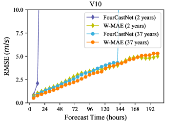
We report the mean ACC and RMSE for each of the variables at each forecast time-step and compare them with the corresponding FourCastNet forecasts that use time-matched initial conditions. We present the performance comparisons of W-MAE and FourCastNet under two different training data durations, namely, two years and thirty-seven years. Figure 3 displays the latitude-weighted ACC and RMSE values for our W-MAE model forecasts (indicated by the red line with markers) and the corresponding FourCastNet forecasts (indicated by the blue line with markers).
As depicted in Figure 3, with two years of training data, the W-MAE pre-trained delivers stable and satisfactory performance in forecasting the future states of multiple meteorological variables. In contrast, FourCastNet exhibits a rapid drop in performance at very short lead times and becomes unable to predict beyond 24 hours. The reason for this is that our W-MAE model, through pre-training, can learn the basic structure and patterns within the data from the limited training data. Subsequently, the pre-trained W-MAE model utilizes the learned fundamental data features which serve as prior knowledge for the model, making it more robust in downstream task fine-tuning. However, traditional models in the case of inadequate training data encounter two limitations: (1) limited capacity to capture latent patterns and features, leading to overfitting or poor performance, and (2) more prone to be affected by noise and outliers, reducing predictive robustness. These limitations may account for the underperformance of FourCastNet.
Under the setting of thirty-seven years of training data, our W-MAE continues to outperform FourCastNet, maintaining stable prediction performance. It is important to note that FourCastNet incorporates a distinct approach to mitigate accumulation errors (see DBLP:journals/corr/abs-2202-11214 for more details), necessitating a second round of training for multi-variable forecasting. To ensure fairness and enable a straightforward comparison, we adopt a first-round-training model of FourCastNet with a training epoch of 150 (matching the count mentioned in FourCastNet). It is observed that the performance of FourCastNet, which lacks the integration of a tailored training process for error accumulation suppression, experiences a significant decline beyond a certain forecast lead time. These findings underscore the superiority of our W-MAE framework in maintaining performance stability and robustness of results. Additionally, in Figure 3, we observe that beyond a certain lead time (approximately 130 hours), the performance of our W-MAE model with thirty-seven years of training data is not as strong as that achieved with two years of training data. This may be attributable to the fact that our W-MAE model with thirty-seven years of training data has not yet converged to its optimal performance. As mentioned in Section 5.1, our W-MAE model with two years of training data undergoes 600 epochs of pre-training, while the model with thirty-seven years of training data is only pre-trained for 200 epochs.
Moreover, we conduct an analysis of the time overhead for fine-tuning our pre-trained W-MAE model in multi-variable forecasting tasks. The fine-tuning process takes 100 epochs, with each epoch lasting an average of 63 minutes on 8 NVIDIA Tesla A800 GPU, resulting in a total fine-tuning time of nearly 105 hours. In comparison, FourCastNet requires 150 epochs of training, averaging 55 minutes per epoch on the same platform resulting in a total training time of around 137 hours. The results indicate that our W-MAE achieves a nearly 23% speedup compared with FourCastNet. This demonstrates that by leveraging the powerful initial parameters provided by pre-training, our W-MAE can achieve fast convergence during the fine-tuning process, which saves training time and computational resources.

5.3 Fine-tuning for precipitation forecasting


Total Precipitation (TP) in the ERA5 dataset is a variable that represents the cumulative liquid and frozen water that falls to the Earth’s surface through rainfall and snowfall. Compared with other meteorological variables, TP presents sparser spatial characteristics. It is calculated from other variables, requiring an intermediate calculation in the derivation process, making it more challenging. For the precipitation forecasting task, we aim to predict the cumulative total precipitation in the next 6 hours using multiple meteorological variables from the previous time-step. We compare the performance of our W-MAE model and FourCastNet using both ACC and RMSE as the evaluation metrics.
Experimental results for different training data settings, i.e. using two years or thirty-seven years of training data, are shown in Figure 5111Note that, only a portion of FourCastNet’s prediction results are displayed in Figure 5. This is because the inability of FourCastNet to make predictions at longer lead times of more than 108 hours for two years of training data. Specifically, our experimental results show that in precipitation forecasting, FourCastNet produces considerable prediction errors beyond a certain lead time, resulting in NAN (not a number) predictions that render the results infeasible.. When using two years of training data, our W-MAE model outperforms FourCastNet in predicting the total precipitation at the 6-hour result. When the training data spans thirty-seven years, at the first forecast time-step (i.e., with a forecast lead time of 6 hours), our model achieves a 20% improvement in terms of the ACC metric compared with FourCastNet (0.996 vs. 0.804). At the 20 forecast time-step (i.e., with a forecast lead time of 5 days), our model significantly outperforms FourCastNet (0.886 vs. 0.234). It is worth noting that despite incorporating the error accumulation suppression optimization techniques and undergoing a second round of training (see DBLP:journals/corr/abs-2202-11214 for detailed training process), the yielding FourCastNet model still exhibits inferior performance in precipitation forecasting compared to our W-MAE model. Moreover, concerning the time costs associated with precipitation forecasting tasks, our W-MAE framework outperforms FourCastNet, with a total training time of 20.6 hours and 23 hours, respectively. These observations suggest that our W-MAE not only achieves superior performance but also reduces the training time, resulting in efficient model training.


5.4 Efficiency of ensemble forecast
The methodology of ensemble forecast mainly involves adding noise to perturb initial weather states and observing the change in forecast results. In this paper, we follow FourCastNet DBLP:journals/corr/abs-2202-11214 to use Gaussian noise to perturb the initial conditions and generate an ensemble of 100 perturbed initial condition sets (represented as =100). The perturbations are scaled by a factor =0.3. We apply large-member ensemble on multi-variable forecasting tasks for . As shown in Figure 6, we compare control forecast (i.e., the unperturbed forecasts) with the mean of a 100-member ensemble forecast using W-MAE. For the short-term forecast time, such as for 1 day, 100-member ensemble forecasts exhibit a slightly lower accuracy than control forecasts by a single model. However, when predicting beyond 5 days, the accuracy of 100-member ensemble forecasts displays a marked improvement compared with control forecasts. This observation affirms that the large-member ensemble forecast is valuable when the precision of individual models is compromised. Moreover, our W-MAE takes an average of 320 ms to infer a 24-hour forecast on one NVIDIA Tesla A800 GPU, which is orders of magnitude faster than traditional NWP methods in ensemble forecast. The results prove the efficiency of our W-MAE on ensemble forecast.
5.5 Ablation study
Effect of pre-training. To fully validate the effectiveness of our method, we apply our pre-training technique to FourCastNet. During the pre-training stage, we set the patch size to (same as that used in FourCastNet), the mask ratio to 0.75, and trained the model for 250 epochs. Then, we fine-tune the pre-trained FourCastNet for the precipitation forecasting task. We compared the performance of the pre-trained FourCastNet with that of the vanilla FourCastNet without pre-training. Our ablation results, as shown in Figure 7, indicate that the pre-trained FourCastNet outperformed FourCastNet without pre-training by nearly 30% in precipitation forecasting when both were trained on two years of data. Moreover, the pre-trained FourCastnet outperformed FourCastNet without pre-training, which was trained on thirty-seven years of data, by nearly 20%. Furthermore, in both training data settings, i.e., using two years and thirty-seven years of training data, FourCastnet with pre-training shows a significant performance improvement compared with that without pre-training. This suggests that applying pre-training to weather forecasting is promising.


Effect of masking ratio. Given the disparity in information density between meteorological images and images in computer vision, we conducted an investigation on the effect of mask ratios on meteorological image reconstruction. Specifically, the training loss under different mask ratios are compared and we set the maximum pre-training epoch to 1000. Figure 8 displays the effect of masking ratios on pixel reconstruction, with the optimal ratio found at approximately 0.6. However, when considering the time overhead of pre-training, we discover that setting the mask ratio to 0.75, compared with 0.6, saves 8% of the computational memory usage and reduces the training time by nearly 4 minutes per epoch. Moreover, the performance of the model at a 0.75 mask ratio can be comparable to that of 0.6. Therefore, to strike a balance between computational efficiency and model performance, we select a mask ratio of 0.75 for model pre-training. Furthermore, Figure 9 visualizes the pixel reconstruction results under varying mask ratio conditions.

6 Conclusion
In this paper, we introduce self-supervised pre-training techniques to the weather forecasting domain, and propose a pre-trained Weather model with Masked AutoEncoder named W-MAE. Our pre-trained W-MAE exhibits stable forecasting results and outperforms the baseline model in longer forecast time-steps. This demonstrates the feasibility and potential of implementing pre-training techniques in weather forecasting. Our study also provides insights for modeling longer-term dependencies (ranging from a month to a year) in the tasks of climate forecasting DBLP:journals/jc/MartinMSBIRK10 ; DBLP:journals/rms/Hoskins13 . We hope that our work will inspire future research on the application of pre-training techniques to a wider range of weather and climate forecasting tasks.
Acknowledgments The authors gratefully acknowledge the support of MindSpore, CANN (Compute Architecture for Neural Networks) and Ascend AI Processor used for this research. The computing infrastructure used in our work is powered by Chengdu Intelligent Computing Center.
Declarations
-
•
Funding This work was supported by the National Natural Science Foundation of China (No. 62276047 and No. 42275009) and CAAI-Huawei MindSpore Open Fund.
-
•
Conflict of interest The authors have no financial or non-financial interests to disclose.
-
•
Ethics approval and Consent to participate The authors declare that this research did not require Ethics approval or Consent to participate since no experiments involving humans or animals have been conducted.
-
•
Consent for publication The authors of this manuscript all consent to its publication.
-
•
Availability of data and materials and Code availability The code and data are available at https://github.com/Gufrannn/W-MAE.
-
•
Authors’ contributions: Conceptualization: Xin Man, Chenghong Zhang; Methodology: Xin Man, Jin Feng, Changyu Li, Jie Shao; Formal analysis and investigation: Xin Man, Chenghong Zhang, Jin Feng, Changyu Li; Writing - original draft preparation: Xin Man; Writing - review and editing: Jin Feng, Jie Shao; Funding acquisition: Jin Feng, Jie Shao.
References
- \bibcommenthead
- (1) Bauer, P., Thorpe, A., Brunet, G.: The quiet revolution of numerical weather prediction. Nature 525(7567), 47–55 (2015)
- (2) Abbe, C.: The physical basis of long-range weather forecasts. Monthly Weather Review 29(12), 551–561 (1901)
- (3) Bjerknes, V.: The problem of weather prediction, considered from the viewpoints of mechanics and physics. Meteorologische Zeitschrift 18(6), 663–667 (2009)
- (4) Schultz, M.G., Betancourt, C., Gong, B., Kleinert, F., Langguth, M., Leufen, L.H., Mozaffari, A., Stadtler, S.: Can deep learning beat numerical weather prediction? Philosophical Transactions of the Royal Society A 379(2194), 20200097 (2021)
- (5) Irrgang, C., Boers, N., Sonnewald, M., Barnes, E.A., Kadow, C., Staneva, J., Saynisch-Wagner, J.: Towards neural earth system modelling by integrating artificial intelligence in earth system science. Nat. Mach. Intell. 3(8), 667–674 (2021)
- (6) Robert, A.: A semi-lagrangian and semi-implicit numerical integration scheme for the primitive meteorological equations. Journal of the Meteorological Society of Japan. Ser. II 60(1), 319–325 (1982)
- (7) Tóth, Z., Talagrand, O., Candille, G., Zhu, Y.: Probability and ensemble forecasts. In: Jolliffe, I.T., Stephenson, D.B. (eds.) Forecast Verification: A Practitioner’s Guide in Atmospheric Sciences, pp. 137–164. John Wiley and Sons, Chichester (2003)
- (8) Leutbecher, M., Palmer, T.N.: Ensemble forecasting. J. Comput. Phys. 227(7), 3515–3539 (2008)
- (9) Chattopadhyay, A., Mustafa, M., Hassanzadeh, P., Bach, E., Kashinath, K.: Towards physically consistent data-driven weather forecasting: Integrating data assimilation with equivariance-preserving deep spatial transformers. CoRR abs/2103.09360 (2021)
- (10) Racah, E., Beckham, C., Maharaj, T., Kahou, S.E., Prabhat, Pal, C.: Extremeweather: A large-scale climate dataset for semi-supervised detection, localization, and understanding of extreme weather events. In: Advances in Neural Information Processing Systems 30: Annual Conference on Neural Information Processing Systems 2017, December 4-9, 2017, Long Beach, CA, USA, pp. 3402–3413 (2017)
- (11) Biswas, M., Dhoom, T., Barua, S.: Weather forecast prediction: An integrated approach for analyzing and measuring weather data. International Journal of Computer Applications 182(34), 20–24 (2018)
- (12) Semenov, M.A., Brooks, R.J., Barrow, E.M., Richardson, C.W.: Comparison of the wgen and lars-wg stochastic weather generators for diverse climates. Climate research 10(2), 95–107 (1998)
- (13) Castro, R., Souto, Y.M., Ogasawara, E.S., Porto, F., Bezerra, E.: Stconvs2s: Spatiotemporal convolutional sequence to sequence network for weather forecasting. Neurocomputing 426, 285–298 (2021)
- (14) Han, J., Liu, H., Zhu, H., Xiong, H., Dou, D.: Joint air quality and weather prediction based on multi-adversarial spatiotemporal networks. In: Thirty-Fifth AAAI Conference on Artificial Intelligence, AAAI 2021, Virtual Event, February 2-9, 2021, pp. 4081–4089 (2021)
- (15) Park, S.K., Xu, L. (eds.): Data Assimilation for Atmospheric, Oceanic and Hydrologic Applications (Vol. II). Springer, Berlin (2013)
- (16) Esener, İ.I., Yüksel, T., Kurban, M.: Short-term load forecasting without meteorological data using ai-based structures. Turkish Journal of Electrical Engineering and Computer Sciences 23(2), 370–380 (2015)
- (17) Albu, A., Czibula, G., Mihai, A., Czibula, I.G., Burcea, S., Mezghani, A.: Nextnow: A convolutional deep learning model for the prediction of weather radar data for nowcasting purposes. Remote. Sens. 14(16), 3890 (2022)
- (18) Dewitte, S., Cornelis, J., Müller, R., Munteanu, A.: Artificial intelligence revolutionises weather forecast, climate monitoring and decadal prediction. Remote Sensing 13(16), 3209 (2021)
- (19) Diao, L., Niu, D., Zang, Z., Chen, C.: Short-term weather forecast based on wavelet denoising and catboost. In: 2019 Chinese Control Conference (CCC), pp. 3760–3764 (2019)
- (20) Devlin, J., Chang, M., Lee, K., Toutanova, K.: BERT: pre-training of deep bidirectional transformers for language understanding. In: Proceedings of the 2019 Conference of the North American Chapter of the Association for Computational Linguistics: Human Language Technologies, NAACL-HLT 2019, Minneapolis, MN, USA, June 2-7, 2019, Volume 1 (Long and Short Papers), pp. 4171–4186 (2019)
- (21) Huang, H., Liang, Y., Duan, N., Gong, M., Shou, L., Jiang, D., Zhou, M.: Unicoder: A universal language encoder by pre-training with multiple cross-lingual tasks. In: Proceedings of the 2019 Conference on Empirical Methods in Natural Language Processing and the 9th International Joint Conference on Natural Language Processing, EMNLP-IJCNLP 2019, Hong Kong, China, November 3-7, 2019, pp. 2485–2494 (2019)
- (22) Li, G., Duan, N., Fang, Y., Gong, M., Jiang, D.: Unicoder-vl: A universal encoder for vision and language by cross-modal pre-training. In: The Thirty-Fourth AAAI Conference on Artificial Intelligence, AAAI 2020, The Thirty-Second Innovative Applications of Artificial Intelligence Conference, IAAI 2020, The Tenth AAAI Symposium on Educational Advances in Artificial Intelligence, EAAI 2020, New York, NY, USA, February 7-12, 2020, pp. 11336–11344 (2020)
- (23) Tian, F., Gao, Y., Fang, Z., Fang, Y., Gu, J., Fujita, H., Hwang, J.: Depth estimation using a self-supervised network based on cross-layer feature fusion and the quadtree constraint. IEEE Trans. Circuits Syst. Video Technol. 32(4), 1751–1766 (2022)
- (24) Li, Y., Gao, Y., Chen, B., Zhang, Z., Lu, G., Zhang, D.: Self-supervised exclusive-inclusive interactive learning for multi-label facial expression recognition in the wild. IEEE Trans. Circuits Syst. Video Technol. 32(5), 3190–3202 (2022)
- (25) Dosovitskiy, A., Beyer, L., Kolesnikov, A., Weissenborn, D., Zhai, X., Unterthiner, T., Dehghani, M., Minderer, M., Heigold, G., Gelly, S., Uszkoreit, J., Houlsby, N.: An image is worth 16x16 words: Transformers for image recognition at scale. In: 9th International Conference on Learning Representations, ICLR 2021, Virtual Event, Austria, May 3-7, 2021 (2021)
- (26) He, K., Chen, X., Xie, S., Li, Y., Dollár, P., Girshick, R.B.: Masked autoencoders are scalable vision learners. In: IEEE/CVF Conference on Computer Vision and Pattern Recognition, CVPR 2022, New Orleans, LA, USA, June 18-24, 2022, pp. 15979–15988 (2022)
- (27) Rasp, S., Thuerey, N.: Data-driven medium-range weather prediction with a resnet pretrained on climate simulations: A new model for weatherbench. Journal of Advances in Modeling Earth Systems 13(2), 2020–002405 (2021)
- (28) Vaswani, A., Shazeer, N., Parmar, N., Uszkoreit, J., Jones, L., Gomez, A.N., Kaiser, L., Polosukhin, I.: Attention is all you need. In: Advances in Neural Information Processing Systems 30: Annual Conference on Neural Information Processing Systems 2017, December 4-9, 2017, Long Beach, CA, USA, pp. 5998–6008 (2017)
- (29) Faisal, A.N.M.F., Rahman, A., Habib, M.T.M., Siddique, A.H., Hasan, M., Khan, M.M.: Neural networks based multivariate time series forecasting of solar radiation using meteorological data of different cities of bangladesh. Results in Engineering 13, 100365 (2022)
- (30) Hersbach, H., Bell, B., Berrisford, P., Hirahara, S., et al.: The era5 global reanalysis. Quarterly Journal of the Royal Meteorological Society 146(730), 1999–2049 (2020)
- (31) Pathak, J., Subramanian, S., Harrington, P., Raja, S., Chattopadhyay, A., Mardani, M., Kurth, T., Hall, D., Li, Z., Azizzadenesheli, K., Hassanzadeh, P., Kashinath, K., Anandkumar, A.: Fourcastnet: A global data-driven high-resolution weather model using adaptive fourier neural operators. CoRR abs/2202.11214 (2022)
- (32) Lam, R., Sanchez-Gonzalez, A., Willson, M., Wirnsberger, P., Fortunato, M., Pritzel, A., Ravuri, S.V., Ewalds, T., Alet, F., Eaton-Rosen, Z., Hu, W., Merose, A., Hoyer, S., Holland, G., Stott, J., Vinyals, O., Mohamed, S., Battaglia, P.W.: Graphcast: Learning skillful medium-range global weather forecasting. CoRR abs/2212.12794 (2022)
- (33) Bi, K., Xie, L., Zhang, H., Chen, X., Gu, X., Tian, Q.: Pangu-weather: A 3d high-resolution model for fast and accurate global weather forecast. CoRR abs/2211.02556 (2022)
- (34) Rodwell, M.J., Richardson, D.S., Hewson, T.D., Haiden, T.: A new equitable score suitable for verifying precipitation in numerical weather prediction. Quarterly Journal of the Royal Meteorological Society 136(650), 1344–1363 (2010)
- (35) Arakawa, A.: Adjustment mechanisms in atmospheric models. Journal of the Meteorological Society of Japan 75(1B), 155–179 (1997)
- (36) Stensrud, D.J.: Parameterization Schemes: Keys to Understanding Numerical Weather Prediction Models. Cambridge University Press, Cambridge (2007)
- (37) Arakawa, A.: The cumulus parameterization problem: Past, present, and future. Journal of Climate 17(13), 2493–2525 (2004)
- (38) Grenier, H., Bretherton, C.S.: A moist pbl parameterization for large-scale models and its application to subtropical cloud-topped marine boundary layers. Monthly Weather Review 129(3), 357–377 (2001)
- (39) Han, Y., Mi, L., Shen, L., Cai, C.S., Liu, Y., Li, K., Xu, G.: A short-term wind speed prediction method utilizing novel hybrid deep learning algorithms to correct numerical weather forecasting. Applied Energy 312, 118777 (2022)
- (40) Chen, R., Wang, X., Zhang, W., Zhu, X., Li, A., Yang, C.: A hybrid cnn-lstm model for typhoon formation forecasting. GeoInformatica 23, 375–396 (2019)
- (41) Rasp, S., Dueben, P.D., Scher, S., Weyn, J.A., Mouatadid, S., Thuerey, N.: Weatherbench: a benchmark data set for data-driven weather forecasting. Journal of Advances in Modeling Earth Systems 12(11), 2020–002203 (2020)
- (42) Keisler, R.: Forecasting global weather with graph neural networks. CoRR abs/2202.07575 (2022)
- (43) Karevan, Z., Suykens, J.A.K.: Transductive LSTM for time-series prediction: An application to weather forecasting. Neural Networks 125, 1–9 (2020)
- (44) Bougeault, P., Toth, Z., Bishop, C., Brown, B., Burridge, D., et al.: The thorpex interactive grand global ensemble. Bulletin of the American Meteorological Society 91(8), 1059–1072 (2010)
- (45) Guibas, J., Mardani, M., Li, Z., Tao, A., Anandkumar, A., Catanzaro, B.: Adaptive fourier neural operators: Efficient token mixers for transformers. CoRR abs/2111.13587 (2021)
- (46) Loshchilov, I., Hutter, F.: Decoupled weight decay regularization. In: 7th International Conference on Learning Representations, ICLR 2019, New Orleans, LA, USA, May 6-9, 2019 (2019)
- (47) Martin, G.M., Milton, S.F., Senior, C.A., Brooks, M.E., Ineson, S., Reichler, T., Kim, J.: Analysis and reduction of systematic errors through a seamless approach to modeling weather and climate. Journal of Climate 23(22), 5933–5957 (2010)
- (48) Hoskins, B.: The potential for skill across the range of the seamless weather-climate prediction problem: a stimulus for our science. Quarterly Journal of the Royal Meteorological Society 139(672), 573–584 (2013)