Voltage controlled iontronic switches: a computational method to predict electrowetting in hydrophobically gated nanopores

Following the same protocol of our previous work Paulo et al. (2023b), we built a molecular dynamics system for which we want to compute the free energy $F$ and the diffusivity $D$ associated with the number of water molecules $N$ inside a hydrophobic nanopore; $N$ represents the coarse-grained variable which defines the wetting/drying process. The system, represented in Fig. 1, is made of a slab of fixed Lennard-Jones atoms in a fcc arrangement, with lattice spacing 0.35 $nm$, from which a cylindrical nanopore was excavated. This slab is surrounded by water molecules (SPC/E Berendsen et al. (1987)), and the water-solid non-bonded interactions are tuned Camisasca et al. (2020) so that the contact angle is $104^{\circ}$. The nanopore has a diameter of 1.4 $nm$ and a length of 2.8 $nm$. To control the pressure of the system, we used two pistons orthogonal to the pore axis Marchio et al. (2018). The NVT ensemble was sampled using a Nosé–Hoover chains thermostat Martyna et al. (1992) at 310 K with a chain length of 3. A constant and homogeneous electric field is applied across the system $\mathrm{E}=(0,0,E_{z})$, with $z$ being the direction parallel to the pore axis, to mimic a difference of a constant voltage across the membrane $\Phi=E_{z}L_{z}$ Gumbart et al. (2012), $L_{z}$ the length of the MD box.

We use Restrained Molecular Dynamics (RMD) Maragliano and Vanden-Eijnden (2006) to compute the free energy as a function of the pore filling $N$. This is done by adding a harmonic restraint to the physical Hamiltonian $H_{\mathrm{phys}}$ of the system,

$$H_{N}(\bm{r},\bm{p})=H_{\mathrm{phys}}(\bm{r},\bm{p})+\frac{k}{2}\left(N-\tilde{N}(\bm{r})\right)^{2}\,,$$

(1)

where $\bm{r}$ and $\bm{p}$ are the positions and momenta of all the atoms, respectively, $k$ is a harmonic constant (1 kcal/mol), $N$ is the desired number of water molecules in a box centered around the nanopore, and $\tilde{N}$ is computed by counting the number of water molecules in the region highlighted in black in Fig. 1. The counting procedure has been explained in detail in previous work Paulo et al. (2023b). The diffusivity $D(N)$, associated to the filling variable, can be computed within the same framework, being related to the integral of the autocorrelation function of $\tilde{N}$ at a given $N$ Paulo et al. (2023b).

In this section, we explore the effect that a transmembrane voltage has on the free energy profile associated with a given collective variable $\theta$, which in the specific case considered here is the number of water molecules inside the pore, $\theta=N$. Here, the main assumption is that the system is at equilibrium even when applying the voltage. Consider a system described by the vector $\bm{x}$ of positions and momenta of its $M$ particles $\bm{x}=(\bm{r_{1}},\bm{p_{1}},\dots,\bm{r_{M}},\bm{p_{M}})$, with a Hamiltonian made by a “zero voltage” part $H_{0}$ and the contribution of the external voltage $\Phi$

$$H(\bm{x},\Phi)=H_{0}(\bm{x})-Q(\bm{r})\Phi\;,$$

(2)

with $Q$ the displacement charge

$$Q(\bm{r})=\frac{\pi(\bm{r})}{L}\;,$$

(3)

where

$$\pi(\bm{r})=\sum\limits_{i=1}^{M}q_{i}\bm{r}_{i}\cdot\bm{\hat{n}}$$

(4)

is the total dipole moment of the system in the direction $\bm{\hat{n}}$ in which the voltage is applied and $L$ is the extension of the system in the same direction.

The probability density function of the system in the canonical ensemble is then

$$\rho(\bm{x},\Phi)=\frac{1}{Z(\Phi)}e^{-\beta H(\bm{x},\Phi)}\;,$$

(5)

with $Z$ the partition function

$$Z(\Phi)=\int e^{-\beta H(\bm{x},\Phi)}\mathrm{d}\bm{x}\;.$$

(6)

Choosing a collective variable $\theta$ which gives a coarser description of the system, the probability density of that variable is

$$P(\theta,\Phi)=\int\delta\left(\theta-\hat{\theta}(\bm{x})\right)\rho(\bm{x},\Phi)\mathrm{d}\bm{x}=\frac{Z_{\theta}(\theta,\Phi)}{Z(\Phi)}\;,$$

(7)

where $\hat{\theta}(\bm{x})$ is the function which associates the microscopic state to a value of the collective variable, and $Z_{\theta}$ is the partition function restrained to a given value of the collective variable

$$Z_{\theta}(\theta,\Phi)=\int\delta\left(\theta-\hat{\theta}(\bm{x})\right)e^{-\beta H(\bm{x},\Phi)}\mathrm{d}\bm{x}\;.$$

(8)

The associated free energy is

$$F(\theta,\Phi)=-\beta^{-1}\log P(\theta,\Phi)\;,$$

(9)

and its variation with respect to voltage

$$\frac{\partial F(\theta,\Phi)}{\partial\Phi}=-\frac{1}{\beta P(\theta,\Phi)}\frac{\partial P(\theta,\Phi)}{\partial\Phi}\;.$$

(10)

The derivative of the coarse grained probability with respect to voltage is

$$\frac{\partial P(\theta,\Phi)}{\partial\Phi}=\int\delta\left(\theta-\hat{\theta}(\bm{x})\right)\frac{\partial\rho(\bm{x},\Phi)}{\partial\Phi}\mathrm{d}\bm{x}\;,$$

(11)

with

$$\frac{\partial\rho(\bm{x},\Phi)}{\partial\Phi}=\left(\frac{\beta Q(\bm{r})}{Z(\Phi)}-\frac{\mathrm{d}Z}{\mathrm{d}\Phi}\frac{1}{Z(\Phi)^{2}}\right)e^{-\beta H(\bm{x},\Phi)}$$

(12)

and

$$\frac{\mathrm{d}Z(\Phi)}{\mathrm{d}\Phi}=\int\beta Q(\bm{r})e^{-\beta H(\bm{x},\Phi)}\mathrm{d}\bm{x}=\beta Z(\Phi)\left\langle Q\right\rangle_{\Phi}\;.$$

(13)

Hence, we obtain an expression for the derivative of the microscopic probability density with respect to voltage

$$\frac{\partial\rho(\bm{x},\Phi)}{\partial\Phi}=\frac{\beta}{Z(\Phi)}\left(Q(\bm{r})-\left\langle Q\right\rangle_{\Phi}\right)e^{-\beta H(\bm{x},\Phi)}\;,$$

(14)

which can be used to compute the derivative for the coarse grained probability density

$$\frac{\partial P(\theta,\Phi)}{\partial\Phi}=\int\delta\left(\theta-\hat{\theta}(\bm{x})\right)\frac{\beta}{Z(\Phi)}\left(Q(\bm{r})-\left\langle Q\right\rangle_{\Phi}\right)e^{-\beta H(\bm{x},\Phi)}\mathrm{d}\bm{x}\;,$$

(15)

simplifying

$$\frac{\partial P(\theta,\Phi)}{\partial\Phi}=\beta P(\theta,\Phi)\left(\left\langle Q\right\rangle_{\theta,\Phi}-\left\langle Q\right\rangle_{\Phi}\right)\;.$$

(16)

We finally obtain an expression for the first order derivative of the free energy with respect to voltage

$$\frac{\partial F(\theta,\Phi)}{\partial\Phi}=\left\langle Q\right\rangle_{\Phi}-\left\langle Q\right\rangle_{\theta,\Phi}$$

(17)

To obtain the second order derivative,

$$\frac{\partial F(\theta,\Phi)^{2}}{\partial^{2}\Phi}=\frac{\partial\left\langle Q\right\rangle_{\Phi}}{\partial\Phi}-\frac{\partial\left\langle Q\right\rangle_{\theta,\Phi}}{\partial\Phi}\;,$$

(18)

we need to compute the derivative of the expected averages. Consider the generic observable $A$, then:

$$\frac{\partial\left\langle A\right\rangle_{\Phi}}{\partial\Phi}=\int A(\bm{x})\frac{\partial\rho(\bm{x},\Phi)}{\partial\Phi}\mathrm{d}\bm{x}\;,$$

(19)

we can use Eq. \eqrefeq:pdf_derivative

$$\frac{\partial\left\langle A\right\rangle_{\Phi}}{\partial\Phi}=\int\frac{\beta A(\bm{x})}{Z(\Phi)}\left(Q(\bm{r})-\left\langle Q\right\rangle_{\Phi}\right)e^{-\beta H(\bm{x},\Phi)}\mathrm{d}\bm{x}\;,$$

(20)

to obtain eventually

$$\frac{\partial\left\langle A\right\rangle_{\Phi}}{\partial\Phi}=\beta\left(\left\langle AQ\right\rangle_{\Phi}-\left\langle A\right\rangle_{\Phi}\left\langle Q\right\rangle_{\Phi}\right)\;.$$

(21)

Now we can compute the second order derivative of the free energy with respect to voltage

$$\frac{\partial F(\theta,\Phi)^{2}}{\partial^{2}\Phi}=\beta\left(\left\langle Q^{2}\right\rangle_{\Phi}-\left\langle Q\right\rangle^{2}_{\Phi}-(\left\langle Q\right\rangle^{2}_{\theta,\Phi}-\left\langle Q^{2}\right\rangle_{\theta,\Phi})\right)\;.$$

(22)

The free energy dependence on the voltage can be then approximated, up to second order, as:

$$F(\theta,\Phi)=F_{0}(\theta,\Phi_{0})+P_{1}(\theta,\Phi_{0})\Delta\Phi+\frac{1}{2}P_{2}(\theta,\Phi_{0})(\Delta\Phi)^{2}+const(\Phi)\;,$$

(23)

where $\Delta\Phi=(\Phi-\Phi_{0})$, with $\Phi_{0}$ being voltage around which the expansion is done; $P_{1}(\theta,\Phi_{0})=-\left\langle Q\right\rangle_{\theta,\Phi_{0}}$ and $P_{2}(\theta)=-\beta\left(\left\langle Q^{2}\right\rangle_{\theta,\Phi_{0}}-\left\langle Q\right\rangle^{2}_{\theta,\Phi_{0}}\right)$; in the constant we collected all the terms that do not depend on $\theta$, $const(\Phi)=\left\langle Q\right\rangle_{\Phi_{0}}\Delta\Phi+\left(\left\langle Q^{2}\right\rangle_{\Phi_{0}}-\left\langle Q\right\rangle^{2}_{\Phi_{0}}\right)\left(\Delta\Phi\right)^{2}$. While this framework is valid for a generic collective variable $\theta$, in the following, we will focus only on the case where the collective variable is the pore filling $N$. During the restrained molecular dynamics simulations used to compute the free energy profiles, we computed also the values of $P_{1}$ and $P_{2}$ for different filling levels and different applied voltages.

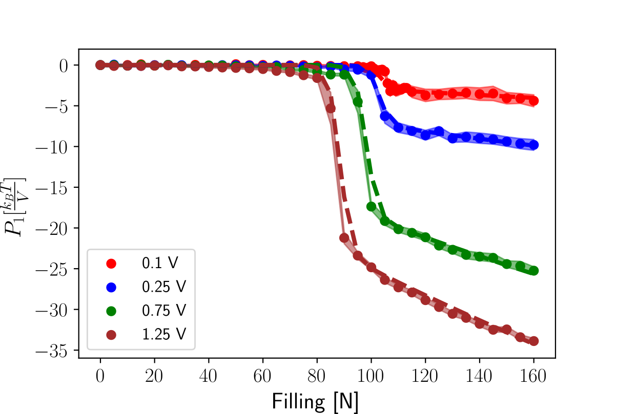
During the restrained molecular dynamics simulations used to compute the free energy, we computed the average displacement charge $\langle Q\rangle_{\theta,0}$ and its second moment,$-\left(\left\langle Q^{2}\right\rangle_{\theta,\Phi_{0}}-\left\langle Q\right\rangle^{2}_{\theta,\Phi_{0}}\right)$, which we then use to compute $P_{1}$ and $P_{2}$ in Eq. \eqrefeq:theory_free as a function of the water filling of the pore; data are reported in Fig. 2. Because the pore shown in Fig. 1 is i) symmetric, ii) uncharged, and iii) the displacement charge enters as a factor proportional to the voltage, $P_{1}$ should not depend on the filling of the pore, as positive and negative voltages must have the same effect on wetting and drying. This argument is backed up by the MD results showing that indeed $P_{1}$ fluctuates around a constant value (Fig. 2a). Differently, the amplitude of the fluctuation of $P_{1}$ sharply increases after a certain filling level, see panel b reporting the value of the second order coefficient $P_{2}$. We related this effect to the fact that the number of fluctuating dipoles (the water molecules) inside the pore is increasing, passing from nearly vacuum (dry) to a much complex situation in which a larger number of molecules is present that can be potentially affected by the external electric field (the applied voltage drop would mainly occur inside the nanopore). Indeed, $P_{2}$ has the dimensions of a capacitance, so the second term added to the free energy could be related to the energy stored in the pore, considering it as a capacitor. In particular, the change in the stored energy depends on the filling medium: the wet pore is filled with water (relative permittivity $\epsilon_{r}\gg 1$), while the dry pore is filled with vapour (i.e., for such confined geometry, vacuum with $\epsilon_{r}\sim 1$). Hence, the capacitance of the dry pore has to be lower than the wet pore; we show by a dashed line what should be the energy of a capacitor with the size of the pore and a relative permittivity $\epsilon_{r}$ of c.a. 40; the latter value is lower than the bulk value due to the extreme confinement, in agreement with what has been reported for pores of sizes similar to the one studied here Dzubiella and Hansen (2005).

The fact that $P_{1}$ is constant and only $P_{2}$ depends on the filling level implies that the wetting probability of symmetric hydrophobic nanopores would depend only on the square of the applied voltage, and not on any linear term, because it would be the only influence on the wetting free energy, in line with what has been reported by other authors Trick et al. (2017).

We computed the free energy $F(N,\Phi)$ and the state dependent diffusivity $D(N,\Phi)$ as a function of pore filling $N$ at different applied voltages $\Phi$ using RMD, see Fig. 3.

We remark that the free energy of a dynamical system is an equilibrium (different from steady state) quantity, hence the protocol used here is strictly valid only in the absence of electric or mass currents. The fluid in the system of Fig. 1 does not include free ions, hence our system reaches equilibrium under every applied voltage and filling constraints. Thus, the quantity we are computing corresponds to the free energy of the system, despite the applied electric field. Figure 3a shows that voltage has a non-linear effect on the free energy of the wet state. Applying $\Phi=0.5$ V changes the free energy difference between the wet and dry state by less than $5\,k_{B}T$ while $\Phi=1$ V changes this difference by more than $15\,k_{B}T$ and $\Phi=1.5$ V by more than $30\,k_{B}T$. The non-linear effect of voltage in wetting of hydrophobic pores has been shown previously Trick et al. (2017) and it is in line with the prediction of our electrowetting theory, Eq. \eqrefeq:theory_free – as it will be shown in Fig. 4 and 5. We note that the position of the free energy barrier changes with applied voltage, meaning that the volume (and possibly shape) of the critical nucleation bubble changes with applied voltage, requiring higher bubble volumes (corresponding to lower filling $N$) to make the pore dry. Panel b shows that the minimum of the diffusivity follows the maximum of the free energy barrier, shifting to lower filling levels as the voltage increases. Instead, differently from what was previously shown for different pressures Paulo et al. (2023b), the magnitude of the diffusivity of the filling variable changes with applied voltage.

We then compared the free energy profiles computed using RMD and the ones predicted by the expansion presented in Eq. \eqrefeq:theory_free with respect to $\Phi_{0}=0$, see Fig. 4. Panels a-d show the theoretical prediction at different voltages, $\Delta\Phi=0.5$, 1, 1.5 and -1 V, using $F_{0}(N,\Phi_{0}=0)$ and the values of $P_{1}(N,\Phi_{0}=0)$ and $P_{2}(N,\Phi_{0}=0)$ shown in Fig. 2. A fair agreement is found for the lowest voltage, $\Delta\Phi=0.5$ V. However, as expected, the discrepancy becomes larger as the applied voltages increases. More specifically, the free energy differences between the wet and dry states are still well predicted at every voltage (within the estimated error) but the free energy barriers are significantly overestimated by Eq. \eqrefeq:theory_free. Moreover, the location of the free-energy maximum does not match the correct filling level $N$ for $\Delta\Phi>0.5$ V. Both simulations and the predicted energy profile show that positive and negative voltages have similar free energy profiles, see Fig. 4b,d.

The main source of error in the prediction stems from the fact that both $P_{1}$ and $P_{2}$ depend on voltage. Indeed, it is possible to improve the accuracy of the free energy prediction by computing $F$, $P_{1}$ and $P_{2}$ at voltages closer to the predicted one, which is equivalent to performing the Taylor expansion in Eq. \eqrefeq:theory_free at larger voltages, i.e., using $F_{0}=F_{0}(N,|\Phi_{0}|>0)$ and corresponding $P_{1}$ and $P_{2}$. As an example, in Fig. 5a,b we compared the prediction of Eq. \eqrefeq:theory_free at $\Phi=1$ V and 1.5 V, respectively, with that computed with RMD, starting from different $F_{0}$. In panel a are shown the predictions of $F(N,\Phi=1V)$ by using $F_{0}$, $P_{1}$ and $P_{2}$ computed – by RMD – at $\Phi_{0}=0$ V (blue) and $\Phi_{0}=0.75$ V (orange); in panel b the prediction for $F(N,\Phi=1.5V)$ is done by using $F_{0}$, $P_{1}$ and $P_{2}$ measured at $\Phi_{0}=0$ V (blue) and $\Phi_{0}=1.25$ V (orange). In both cases, as expected, the theoretical expansion at smaller $\Delta\Phi=\Phi-\Phi_{0}$ gives much closer predictions to the the free energy computed by RMD. Panels Fig. 5c,d quantify the differences between the profiles shown in the panels a and b, respectively, for each filling level $N$. In both panels, it is possible to see that the largest error comes from the free energy barrier separating the wet and dry states. The insets in both panels show how the maximum difference between the free energies lowers as the theoretical expansion is performed closer to the predicted voltage, being as low as 2 $k_{B}T$ for a difference $\Delta\Phi\sim 0.25$ V.

Both $P_{1}$ and $P_{2}$ depend on the applied voltage, see Fig. 6. $P_{1}$ is symmetric with respect to the applied voltage, see the green ($1$ V) and violet ($-1$ V) lines in Fig. 6a. The symmetry of $P_{1}$ comes from the symmetry of the system, hence positive and negative applied voltages must have the same effect on the free energy, i.e. it must be that: $\Phi\;P_{1}(N,\Phi)=-\Phi\;P_{1}(N,-\Phi)$. Moreover, $P_{1}(\Phi,N)$ cannot be everywhere constant for voltages different from 0. Indeed, consider the free energy profile of the system at $\Phi=1$ V: in that case, applying a voltage difference of $+1$ V or $-1$ V must give different results, because in one case you would be considering the free energy profile at 2 V, while the other you would be considering the free energy profile at 0 V.

$P_{1}$ is related to the dipole moment of the liquid inside the pore, and the interpretation of Fig. 6a is that the polarization of the liquid phase is higher than that of the vapour phase, as previously discussed, with a discontinuous jump close to the transition state. It is also possible to observe an increase of $P_{1}$ in the wet state (as $N$ increases), with the slope depending on the applied voltage. Indeed, a larger electric field will make the water molecules more ordered, and so the total dipole moment of the liquid inside the pore will increase with the voltage; moreover, the number of ordered dipoles increases with the number of water molecules filling the pore.

On the other hand, $P_{2}$ has the same value for positive and negative voltages, see Fig. 6b. As previously discussed, $P_{2}$ has the units of a capacitance and is observed to increase with the filling $N$ in the wet state and to decrease with the applied voltage. Using the same analogy of the capacitor, this must mean that the dielectric constant of the medium goes down (as the distance and area of the plates remains the same). This result is in line with previously reported data from atomistic simulations in hydrophobic nanopores, showing that the relative permittivity of water decreases with applied electric field Dzubiella and Hansen (2005); this is linked to the disruption of the hydrogen bond network under confinement.

As we previously demonstrated, for this particular system, our second order expansion leads to errors lower than ca. $5\,{k_{B}T}$ on the barrier only for $\Delta\Phi\leq 0.5$ V; this error is not negligible when predicting the wetting and drying rates of an hydrophobically gated switch. However, it is impractical to compute $P_{1}$ and $P_{2}$ for multiple applied voltages, because this requires computationally expensive RMD simulations. Because $P_{1}=\frac{dF}{d\Phi}$, we tried to find a phenomenological formula for $P_{1}(N,\Phi)$, which would allow us to compute directly the free energy at any $\Phi$ by integrating the expression.

To model $P_{1}$ we consider that its expression should contain some switching function that changes from a low value to a high value at a critical filling level $N^{*}$. This critical value depends on the applied voltage, and so we write it as $N^{*}(\Phi)$. The switching function chosen by us is a sigmoid, with expression $\frac{a(\Phi)}{1+e^{-1/2(N-N^{*}(\Phi))}}$, with $a(\Phi)$ representing a voltage-dependent amplitude. This expression does not completely capture the behaviour of $P_{1}$, in particular, its increase in absolute value at higher fillings, see Fig. 6a. In order to capture this trend, one can multiply the described switching function by $N^{2/3}$. This left us to determine the expression of $a(\Phi)$, $b(\Phi)$, and $N^{*}(\Phi)$, which we modelled as $a=a_{0}\tanh(\Phi)$, $b=1/2$, and $N^{*}=N_{0}-c|\Phi|$. The final expression for $P_{1}$ has the form:

$$P_{1}(N,\Phi)=\frac{a_{0}\tanh(\Phi)N^{2/3}}{1+e^{-\frac{(N-N_{0}+c|\Phi|)}{2}}},$$

(24)

see the supplementary materials for the fitting involved in the determination of the appropriate constants, $N_{0}$, $c$, $a_{0}$. The agreement between that expression and voltages not used in the fitting is shown in Fig. 7.

The fitted phenomenological expression is rigorously only applicable to the specific system shown in Fig. 1. Currently, this expression is not dimensionally coherent, and we believe this expression is not a general one, especially for more complex systems, but it reasonably describes the shapes of $P_{1}$ at different voltages. Further work is needed to clarify if a more general, physically informed expression of this function exists. We believe that the arguments presented here can anyway help as guidance to fit similar phenomenological expressions in other systems, effectively speeding up the estimation of the free energy at any voltage using a minimal set of RMD simulations.

Having access to an analytical form of $P_{1}$ means that we can reconstruct the free energy profile at any voltage, by integrating $P_{1}$ and adding this value to the free energy at $\Phi=0$, see Fig. 8a. This approach leads to a much more accurate estimation of the free energy profile than that of Fig. 4, with the maximum error at free energy barrier being less than 2 $k_{B}T$, see Fig. 8b. Despite the fact that this protocol can be used to generate the free energy profile at arbitrary voltages, we believe that extrapolations higher than $\Delta\Phi\gg 1.5$ V will most likely give unphysical results.

With the idea of iontronic switches in mind, we compute the wetting and drying times at different voltages by using a rate theory expression Hänggi et al. (1990) fed with the free energy profile $F(N,\Phi)$ and the state dependent diffusivity $D(N,\Phi)$:

$$t_{w}(\Phi)=\int_{N_{d}}^{N_{w}}\frac{e^{\frac{F(N,\Phi)}{k_{B}T}}}{D(N,\Phi)}dN\;\int_{N_{d}}^{N_{w}}e^{\frac{-F(N,\Phi)}{k_{B}T}}\left(\int_{N_{d}}^{N}\frac{e^{\frac{F(N,\Phi)}{k_{B}T}}}{D(N,\Phi)}dN^{\prime}\right)dN,$$

(25)

with $t_{w}$ being the wetting time and $N_{d}$ and $N_{w}$ the filling levels of the dry and wet states. To compute the drying time, one just needs to switch the integration limits. The wetting and drying rates are then computed as the inverse of the wetting and drying times, respectively. We plot the results of these calculations in Fig. 9. We observe a complete inversion of the gating behaviour when voltage is applied. At low applied voltages, the system dries, i.e., switches off, much faster than it spontaneously wets, meaning that it mostly stays in the dry state. As voltage increases the wetting rate increases, but it is still lower than $1~{}\mu s^{-1}$ up to an applied voltage of 1 V. For higher voltages, the drying rate becomes much smaller than the wetting rate, because the probability of the system being in the wet state is given by $P_{w}=\frac{r_{w}}{r_{w}+r_{d}}$, where $r_{w}$ and $r_{d}$ are the wetting and dryng rates. The wet state of the pore is conductive to ions, while the dry state is not, which means that voltage can be used to switch the system from a conductive to a non-conductive state, and vice-versa.

References

- Vincent et al. (2006) J. F. Vincent, O. A. Bogatyreva, N. R. Bogatyrev, A. Bowyer, and A.-K. Pahl, Journal of the Royal Society Interface 3, 471 (2006).
- Bhushan (2009) B. Bhushan, Philosophical Transactions of the Royal Society A: Mathematical, Physical and Engineering Sciences 367, 1445 (2009).
- Arbring Sjöström et al. (2018) T. Arbring Sjöström, M. Berggren, E. O. Gabrielsson, P. Janson, D. J. Poxson, M. Seitanidou, and D. T. Simon, Advanced Materials Technologies 3, 1700360 (2018).
- Gidon et al. (2020) A. Gidon, T. A. Zolnik, P. Fidzinski, F. Bolduan, A. Papoutsi, P. Poirazi, M. Holtkamp, I. Vida, and M. E. Larkum, Science 367, 83 (2020).
- Hille (1970) B. Hille, Progress in biophysics and molecular biology 21, 1 (1970).
- MacAulay (2021) N. MacAulay, Nature Reviews Neuroscience 22, 326 (2021).
- Lynch et al. (2020) C. I. Lynch, S. Rao, and M. S. Sansom, Chemical Reviews 120, 10298 (2020).
- Roux et al. (2004) B. Roux, T. Allen, S. Bernèche, and W. Im, Quarterly Reviews of Biophysics 37, 15 (2004).
- Corry and Chung (2006) B. Corry and S.-H. Chung, Cellular and Molecular Life Sciences CMLS 63, 301 (2006).
- Almers (2005) W. Almers, Reviews of Physiology, Biochemistry and Pharmacology, Volume 82 , 96 (2005).
- Bezanilla (2008) F. Bezanilla, Neuron 60, 456 (2008).
- Hodgkin and Huxley (1952) A. L. Hodgkin and A. F. Huxley, The Journal of physiology 117, 500 (1952).
- Bassetto Jr et al. (2023) C. A. Bassetto Jr, F. Costa, C. Guardiani, F. Bezanilla, and A. Giacomello, Nature Communications 14, 1110 (2023).
- Furini and Domene (2012) S. Furini and C. Domene, PLoS computational biology 8, e1002476 (2012).
- Xiong et al. (2023) T. Xiong, C. Li, X. He, B. Xie, J. Zong, Y. Jiang, W. Ma, F. Wu, J. Fei, P. Yu, and L. Mao, Science 379, 156 (2023).
- Najem et al. (2018) J. S. Najem, G. J. Taylor, R. J. Weiss, M. S. Hasan, G. Rose, C. D. Schuman, A. Belianinov, C. P. Collier, and S. A. Sarles, ACS Nano 12, 4702 (2018).
- Indiveri et al. (2011) G. Indiveri, B. Linares-Barranco, T. J. Hamilton, A. van Schaik, R. Etienne-Cummings, T. Delbruck, S.-C. Liu, P. Dudek, P. Häfliger, S. Renaud, J. Schemmel, G. Cauwenberghs, J. Arthur, K. Hynna, F. Folowosele, S. Saighi, T. Serrano-Gotarredona, J. Wijekoon, Y. Wang, and K. Boahen, Frontiers in Neuroscience 5 (2011), 10.3389/fnins.2011.00073.
- Zhu et al. (2020) J. Zhu, T. Zhang, Y. Yang, and R. Huang, Applied Physics Reviews 7 (2020), 10.1063/1.5118217.
- Xu et al. (2019) Y. Xu, J. Ma, X. Zhan, L. Yang, and Y. Jia, Cognitive Neurodynamics 13, 601 (2019).
- Hegab et al. (2015) A. M. Hegab, N. M. Salem, A. G. Radwan, and L. Chua, International Journal of Bifurcation and Chaos 25, 1530017 (2015).
- Chua et al. (2012) L. Chua, V. Sbitnev, and H. Kim, International Journal of Bifurcation and Chaos 22, 1230011 (2012).
- Brannigan and Wilkinson (2002) J. A. Brannigan and A. J. Wilkinson, Nature Reviews Molecular Cell Biology 3, 964 (2002).
- Huang et al. (2016) P.-S. Huang, S. E. Boyken, and D. Baker, Nature 537, 320 (2016).
- Zhao et al. (2019) S. Zhao, L. Restrepo-Pérez, M. Soskine, G. Maglia, C. Joo, C. Dekker, and A. Aksimentiev, ACS nano 13, 2398 (2019).
- Aryal et al. (2015) P. Aryal, M. S. Sansom, and S. J. Tucker, Journal of molecular biology 427, 121 (2015).
- Giacomello (2023) A. Giacomello, The Journal of Chemical Physics 159 (2023).
- Lippmann et al. (1875) G. Lippmann et al., Ann. Chim. Phys 5, 494 (1875).
- Mugele and Baret (2005) F. Mugele and J.-C. Baret, Journal of Physics: Condensed Matter 17, R705 (2005).
- Dzubiella and Hansen (2005) J. Dzubiella and J.-P. Hansen, The Journal of Chemical Physics 122 (2005), 10.1063/1.1927514.
- Vanzo et al. (2014) D. Vanzo, D. Bratko, and A. Luzar, The Journal of Physical Chemistry B 119, 8890 (2014).
- Klesse et al. (2020) G. Klesse, S. J. Tucker, and M. S. P. Sansom, ACS Nano 14, 10480 (2020).
- Powell et al. (2011) M. R. Powell, L. Cleary, M. Davenport, K. J. Shea, and Z. S. Siwy, Nature Nanotechnology 6, 798 (2011).
- Smirnov et al. (2011) S. N. Smirnov, I. V. Vlassiouk, and N. V. Lavrik, ACS Nano 5, 7453 (2011).
- Polster et al. (2022) J. W. Polster, F. Aydin, J. P. de Souza, M. Z. Bazant, T. A. Pham, and Z. S. Siwy, Journal of the American Chemical Society 144, 11693 (2022).
- Paulo et al. (2023a) G. Paulo, K. Sun, G. di Muccio, A. Gubbiotti, B. M. della Rocca, J. Geng, G. Maglia, M. Chinappi, and A. Giacomello, “Hydrophobically gated memristive nanopores for neuromorphic applications,” (2023a).
- Humphrey et al. (1996) W. Humphrey, A. Dalke, and K. Schulten, Journal of molecular graphics 14, 33 (1996).
- Paulo et al. (2023b) G. Paulo, A. Gubbiotti, and A. Giacomello, The Journal of Chemical Physics 158 (2023b), 10.1063/5.0147647.
- Berendsen et al. (1987) H. Berendsen, J. Grigera, and T. Straatsma, Journal of Physical Chemistry 91, 6269 (1987).
- Camisasca et al. (2020) G. Camisasca, A. Tinti, and A. Giacomello, The Journal of Physical Chemistry Letters 11, 9171 (2020).
- Marchio et al. (2018) S. Marchio, S. Meloni, A. Giacomello, C. Valeriani, and C. Casciola, The Journal of chemical physics 148, 064706 (2018).
- Martyna et al. (1992) G. J. Martyna, M. L. Klein, and M. Tuckerman, The Journal of chemical physics 97, 2635 (1992).
- Gumbart et al. (2012) J. Gumbart, F. Khalili-Araghi, M. Sotomayor, and B. Roux, Biochimica et Biophysica Acta (BBA)-Biomembranes 1818, 294 (2012).
- Maragliano and Vanden-Eijnden (2006) L. Maragliano and E. Vanden-Eijnden, Chemical physics letters 426, 168 (2006).
- Trick et al. (2017) J. L. Trick, C. Song, E. J. Wallace, and M. S. Sansom, ACS nano 11, 1840 (2017).
- Hänggi et al. (1990) P. Hänggi, P. Talkner, and M. Borkovec, Reviews of Modern Physics 62, 251 (1990).