Volatility models in practice: Rough, Path-dependent or Markovian?
Abstract
An extensive empirical study of the class of Volterra Bergomi models using SPX options data between 2011 and 2022 reveals the following fact-check on two fundamental claims echoed in the rough volatility literature:
Do rough volatility models with Hurst index really capture well SPX implied volatility surface with very few parameters? No, rough volatility models are inconsistent with the global shape of SPX smiles. They suffer from severe structural limitations imposed by the roughness component, with the Hurst parameter controlling the smile in a poor way. In particular, the SPX at-the-money skew is incompatible with the power-law shape generated by rough volatility models. The skew of rough volatility models increases too fast on the short end, and decays too slow on the longer end where “negative” is sometimes needed.
Do rough volatility models really outperform consistently their classical Markovian counterparts? No, for short maturities they underperform their one-factor Markovian counterpart with the same number of parameters. For longer maturities, they do not systematically outperform the one-factor model and significantly underperform when compared to an under-parameterized two-factor Markovian model with only one additional calibratable parameter.
On the positive side: our study identifies a (non-rough) path-dependent Bergomi model and an under-parameterized two-factor Markovian Bergomi model that consistently outperform their rough counterpart in capturing SPX smiles between one week and three years with only 3 to 4 calibratable parameters.
- JEL Classification:
-
G13, C63, G10, C45.
- Keywords:
-
SPX options, Stochastic volatility, Pricing, Calibration, Neural Networks
1 Introduction
1.1 Context
In the realm of (rough) volatility modeling, certain claims have gained widespread popularity and acceptance within academic circles and finance community. Specifically, it has been widely disseminated that rough volatility models exhibit exceptional performance, seemingly reproducing the stylized facts of option prices with remarkable precision while utilizing only a limited number of parameters. Furthermore, it has been argued that they outperform their traditional stochastic volatility model counterparts in capturing the essential features of volatility surfaces. These assertions have been made time and again in various research papers and were often presented with a high degree of confidence in contrast with little empirical evidence.
There is undoubtedly mathematical beauty in rough volatility111From the theoretical side, there is no doubt that the rough volatility paradigm has been an inspiring source of motivation that lead to a better understanding of universal mathematical structures for a large class of non-Markovian and non-semimartingale Volterra processes, to cite a few [3, 4, 5, 6, 11, 15, 21, 29, 34, 40, 41, 43, 44, 51]., and “roughness is in the eye of the beholder” certainly sounds poetic. However as mathematicians, it is incumbent upon us to undertake a rigorous examination of these claims before echoing them. First, the assertions about the superior performance of rough volatility models appear to rest heavily on a limited set of visual fits confined to specific dates or time intervals, casting doubt on their applicability across a wider period. Furthermore, there has been notable omission in the literature concerning a fair and comprehensive comparison between rough volatility models and other models, such as the conventional Markovian stochastic volatility models and non-rough path-dependent volatility models. This absence leaves a critical gap in our understanding of the practical usefulness of rough volatility models, as the non-semimartingale and non-Markovian nature of rough volatility models have an important implementation cost that needs to be justified.
Recently, a series of independent empirical studies [7, 22, 38, 50], each focusing on different aspects of the volatility surface, presented evidence against the claim of “superior performance” attributed to rough volatility models in capturing the main characteristics of volatility surfaces. In particular, the following observations were made:
- •
-
•
Rough volatility models underperform, by a clear margin, their one-factor Markovian counterparts in all market conditions for short maturities with the same number of calibratable parameters for the joint SPX-VIX calibration problem [7];
- •
Inspired by these studies, we conducted our own comprehensive empirical study using daily SPX implied volatility surface data from CBOE spanning from 2011 to 2022. Our study integrates various aspects explored in these earlier works and introduces new evidence and arguments to further challenge the perceived superiority of rough volatility models. We examine both the static performance of various models, such as their daily fit to the whole SPX volatility surface and to the ATM skew, as well as their dynamical performance by assessing how well they predict the future implied volatility surface. Moreover, our empirical study is divided into two parts: part one is dedicated to options with short maturities (one week to three months), with part two focusing on options with long maturities (one week to three years). This division offers additional insights into model performances at different timescales which could be useful in practice.
The empirical experiments in this paper are designed to ensure the comparison between various models is as fair as possible. To this end, we selected models from the same family of Volterra Bergomi models where the volatility process is driven by rough, path-dependent (non-rough semimartingale) and Markovian factors. The models we ended up with have (almost) the same number of calibratable parameters that can be interpreted in a similar way. Furthermore, the same daily forward variance curves extracted from market data are shared among all models for consistency.
As closed-form expression for option pricing under the family of Volterra Bergomi models are unavailable, we calibrate all models to market data using the generic unified numerical method ‘deep pricing with quantization hints’ developed in [7] based on functional quantization as a first proxy with Neural Networks (NN) as a corrector. Compared to other neural network structures used for pricing and calibration [42, 50], this method features significantly lower input dimensions (i.e. the forward variance curve of the Bergomi model is not part of the NN input). In addition, it is free from butterfly arbitrage by construction and mesh-free, allowing one to price derivatives for any strike and maturity combination without interpolation or extrapolation. Notably, this method also allows us to calibrate each model to the market ATM skew without relying on the approximation formula of the Bergomi-Guyon expansion [14] as in [22, 38]. This leads to a more accurate computation of the skew that is free from higher order error in the Bergomi-Guyon expansion when volatility of volatility (vol of vol) is large.
1.2 What are rough volatility models?
Rough volatility models are a specific subclass of non-Markovian stochastic volatility models, where the volatility process is assumed to be a non-semimartingale process characterized by continuous paths rougher than those of standard Brownian motion. Specifically, these models employ variants of fractional Brownian motion with a Hurst index less than 1/2 to model the instantaneous volatility. For instance, in [10], the authors used a Riemann-Louiville fractional Brownian motion given by:
| (1.1) |
where is a standard Brownian motion to describe the spot volatility process. The Hurst index governs the local regularity of the path of , indicating that is Hölder continuous of order strictly less than . In the special case of , the process reduces to classical Brownian motion. The restriction ensures that the convolution kernel is locally square-integrable so that the stochastic integral is well-defined as an Itô integral.
The Riemann-Liouville fractional Brownian motion (1.1) with is non-Markovian, as it represents a weighted average of the increments of Brownian motion by the kernel . It is non-semimartingale due to the singularity of the kernel at , since . While historical volatility exhibits many path-dependent features such as volatility clustering, feedback and memory effects, and multiple timescales [18, 23, 39, 45, 47, 48], the raison d’être of the rough volatility paradigm is to posit that high fluctuations and erratic/spiky behavior observed in volatility on short timescales arise from a rough continuous non-semimartingale process.
To support the necessity of rough volatility and non-semimartingality, two empirical arguments were presented. First, the logarithm of realized volatility time series for various equity market indices exhibits statistical “rougher” trajectories (lower Hölder regularity) compared to standard Brownian motion [33]. An earlier but less popular empirical study of the roughness of the realized volatility appeared in [20] to motivate the need of a rough multi-fractional Brownian motion. Second, authors in [10, 17, 27, 31, 33] argued that market ATM skew term structure exhibits power law decay that explodes in the short term, a phenomenon that rough volatility models can reproduce [9, 10, 30].
However, the validity of both empirical arguments hinges on exceedingly fine timescales that are impractical to attain in finite data sets. Regarding the statistical roughness observed in the realized volatility time series, two independent studies [1, 49] as early as 2018 demonstrated that fast mean-reverting continuous semi-martingales can produce spurious roughness at any realistic timescale, see also some more recent studies [19, 39] and Section 5.2 below. Recently, challenges to the claimed explosiveness of the short end of the ATM skew have been raised in [22, 38].
Setting aside the debate, one of our goals is to assess whether the inherent rough non-semimartingale component in rough volatility models, i.e. the explosiveness of the kernel at , aligns convincingly with market volatility surfaces across short and longer maturities as claimed in the rough volatility literature. It is crucial to emphasize that questioning a rough volatility model involves challenging its non-semimartingality, i.e. the explosion of the kernel at , rather than disputing its non-Markovian path-dependent nature. Said differently: are rough volatility models the ‘good’ non-Markovian models in practice?
1.3 Do rough volatility models really outperform significantly their classical Markovian counterparts?
This paper looks into two main aspects of model performance. First is the static aspect, measured by how accurate a model fits to the market smiles and ATM skew. Second is the dynamical aspect, measured by how well a model predicts future implied volatility.
Fitting short maturities between one week to three months: our empirical study shows that the rough Bergomi model actually underperforms on average compared to the one-factor Bergomi (Markovian) model with the same number of model parameters in fitting the volatility surface and the ATM skew. The one-factor Bergomi is also slightly better in predicting future volatility surface. In other words, there is clearly no advantage in using rough volatility models over classical Markovian models in the short term.
Fitting longer maturities between one week to three years: the rough Bergomi and the one-factor Bergomi models produce equally poor fits and are inconsistent with the SPX smiles, although the one-factor Bergomi model seems to at least be able to achieve a curved shape for the ATM skew in log-log plot more representative of the market, versus the straight line of rough volatility models. The rough Bergomi model slightly, but not consistently, outperforms the one-factor (Markovian) Bergomi model in fitting the volatility surface on average, but scores the highest variance. For the period between 2017 to 2019, the rough Bergomi model underperforms the one-factor Bergomi model. Furthermore, the rough Bergomi model significantly underperforms across all aspects compared to an under-parameterized two-factor (Markovian) Bergomi model with just one-extra calibratable parameter.
1.4 Do rough volatility models with Hurst index really capture SPX smiles with very few parameters?
Our study shows that rough volatility models are inconsistent with the global SPX volatility surface, caused by their severe structural limitations. In particular, the SPX ATM skew term structure cannot be modeled by the rigid power-law shape generated by rough volatility models. When one zooms in on the short end of the volatility surface, the SPX ATM skew does not increase as fast as that of rough volatility models, in line with [22, 38]. In addition, the power law decay for long maturities observed on the market appears to be faster than on average. Specifically, the average speed of decay of the ATM skew for large maturities over the last decade implies a negative value of which is impossible for rough volatility models, since their is constrained above zero.
On the other hand, we show that the path-dependent (non-rough) and the under-parameterized two-factor Bergomi model have no problem capturing the entire term structure of the SPX smiles and ATM skew via unconstrained and can effectively decouple the short end and the long end of the volatility surface in a parsimonious way, with only 3 to 4 calibratable parameters.
The superior performance of the non-rough path-dependent Bergomi model versus the rough Bergomi model highlights that the problem with rough volatility models seems to come from the non-semimartingale part, i.e. singularity of the kernel at . Indeed, the non-rough path-dependent model is obtained by smoothing out the singularity of the fractional kernel at using a fixed value , which shows that the added flexibility of the path-dependent model comes from eliminating the rough, non-semimartingale behavior of rough volatility models and not from the calibration of an additional parameter. In volatility modelling, path-dependency is a desirable trait allowing a model to be more flexible at capturing several stylized facts of volatility, such as volatility clustering, feedback and memory effects, and multiple timescales. However, the non-semimartingality encoded in rough volatility models via the explosive kernel near seems too restrictive and erodes the flexibility gained from path-dependency. Thus contrary to what is put forward by rough volatility advocates, roughness/non-semimartingality is not a necessary condition for effective volatility modelling. Furthermore, all models in this paper can generate spurious ‘statistical roughness’, see Section 5.2 which suggests that after all, estimation of the roughness of the realized volatility time series might not be sufficient to quantify the erratic and spiky behavior that characterizes the volatility of the market.
Outline of the paper: In Section 2, we will first introduce different Volterra Bergomi models considered in this paper and present their main relevant characteristics. In Section 3, we define the performance metrics used to evaluate model performance and address the specifics associated with model calibration. In Section 4, we present the empirical results on the static model performance in two parts, with part one dedicated to short maturities between one week to three months and part two for longer maturities between one week to three years. In the final Section 5, we compare the dynamical aspect of each model by looking at their prediction performance and estimating the statistical roughness of their simulated volatility paths.
2 The class of Volterra Bergomi models
The general form of the Volterra Bergomi stochastic volatility model for a (forward) stock price with instantaneous variance is defined as:
| (2.1) | ||||
with and . Here is a two-dimensional Brownian motion on a risk-neutral filtered probability space . The process is a centered Gaussian process with a non-negative locally square integrable kernel , in particular , for all . The deterministic input curve allows the model to match certain term structure of volatility (e.g. the forward variance curve):
| (2.2) |
The choice of the kernel defines the dynamics of (e.g. rough, path-dependent or Markovian) and plays a crucial role in the model’s capability of capturing the SPX (or other equity indices) volatility surface. In this paper, We shall consider the following kernels and their corresponding model name in Table 1:
Model name Domain of Semi-mart. Markovian rough ✗ ✗ path-dependent ✓ ✗ one-factor ✓ ✓ two-factor ✓ ✓
To ensure comparability among all models, we fix and . This means that all models contain the same number of calibratable parameters , except the two-factor Bergomi model which takes on an additional calibratable parameter . The fixed values may seem arbitrary, however our goal is not about finding the optimal values for , but rather to compare all models as fairly as possible. Furthermore, fixing to these values does not alter the conclusion of this paper compared to setting these parameters free.
The particular parametrization of the one-factor and two-factor Bergomi models ensures that the parameter has a similar interpretation across all these models. This would become more clear as we introduce each Bergomi model in the sections below.
We now introduce the ATM skew which is an important feature of the SPX volatility surface. The ATM skew is defined as:
where is the implied volatility of vanilla options calculated by inverting the Black-Scholes formula with log-moneyness and maturity . For the purpose of this paper, when we refer to the ATM skew, we would be actually referring to the negative value of .
2.1 The rough Bergomi
The rough Bergomi model of [10] defines as:
| (2.3) |
with the vol-of-vol parameter and the Hurst index that coincides with the roughness of the process , i.e. the paths of are Hölder-continuous of any order strictly less than , almost surely. For , the fractional kernel explodes as , so that the process is not a semi-martingale with trajectories rougher than that of standard Brownian motion. The restriction ensures that the kernel is locally square-integrable, so that the stochastic convolution is well-defined as an Itô integral.
2.2 The path-dependent Bergomi
In the path-dependent Bergomi Model, the dynamics of is governed by:
| (2.5) |
The time shifted kernel, , with has been independently introduced over the years in [2, 7, 13, 37]. It represents a small perturbation in the fractional kernel by . However, this shift means is finite, thus allowing the domain of to be extended to while remains integrable. The process is now a semi-martingale and thus the sample paths have the same regularity as standard Brownian motion and are Hölder-continuous of any order strictly less than .
The process is not Markovian. To see this, we apply Itô’s formula and get:
| (2.6) |
Next, with the help of the resolvent of the first kind of , defined as the deterministic measure such that , for all , with , where is a completely monotone function, we get
| (2.7) |
with
| (2.8) |
see [2, Lemma 1.2] for detailed similar computations. is non-Markovian due to the part in the drift which depends on the whole trajectory of up to time , hence the name path-dependent.
The expression (2.7) provides essential insights to the dynamic of the process : for small , one expects the non-Markovian term to be negligible, so that the process behaves locally like an Ornstein-Uhlenbeck process with large mean-reversion speed and vol of vol for small . For large , the non-Markovian term becomes more prominent and introduces path-dependency.
The path-dependent Bergomi model is very different to the rough Bergomi model. It is true that for , by setting in (2.5), one recovers the rough Bergomi model. However for any , the path-dependent Bergomi model produces a distinct model dynamic. This can be seen from its ATM skew formula [35] below in the first order of vol of vol, in contrast to that of the rough Bergomi model in (2.4):
| (2.9) |
This formula shows that the global shape of the ATM skew of the path-dependent Bergomi model is more flexible than the power-law shape of the rough Bergomi model. For very short maturities, the ATM skew of the path-dependent Bergomi model approaches a finite limit which can be made as arbitrarily large as necessary via different values of , in contrast to the blow up to in the rough Bergomi model. For longer maturities, the ATM skew of the path-dependent Bergomi model decays at a rate , with the crucial difference that can be negative, thus allowing the ATM skew to decay faster than that of rough Bergomi model.
For this paper, we fix the value without calibration. This choice not only ensures the same number of calibratable parameters as the rough Bergomi model, but also underscores that the flexibility of the path-dependent model comes from eliminating the rough, non-semimartingale behavior (i.e. removing the singularity of the kernel at ) of rough volatility models and not from the calibration of an additional parameter, as we will see in Section 4.
2.3 The one-factor Bergomi
The one-factor Bergomi model introduced in [12] and [24] models using a standard Ornstein Uhlenbeck process:
| (2.10) |
where . For small and , has a large mean reversion speed of order and a large vol of vol of order . This way of parameterizing is reminiscent of models of fast regimes in [2, 4, 7, 26, 46] and can be seen as a Markovian proxy of the path-dependent Bergomi model from the previous section by dropping the non-Markovian term in (2.7).
This way of parametrization allows to take on a similar interpretation to that in the path-dependent Bergomi model: the more negative the , the statistically rougher the sample path of driven by larger mean reversion and vol-of-vol, see Section 5.2 below. It also allows us to easily compare the models since they have the same calibratable parameters.
The ATM skew produced by the one-factor Bergomi model at first order of vol of vol, assuming a flat is of the from [14]:
| (2.11) |
which shares the same finite limit to that of the path-dependent Bergomi model. For small , the ATM skew decay for both models are similar: a simple computation reveals that both models have the same limit in their first order derivative in with respect to the skew:
| (2.12) |
Therefore we can expect similar model behavior between the path-dependent and one-factor Bergomi models for very short maturities, see Section 4.1. On the other hand, the ATM skew decay of the one-factor Bergomi model is for large .
2.4 The (under-parameterized) two-factor Bergomi
The two factor Bergomi model introduced in [12] contains two Ornstein Uhlenbeck factors and in the instantaneous variance :
| (2.13) |
where the parametrization of both factors are derived in the same way as the one-factor Bergomi model above with .
In the literature, the two factors are usually driven by two correlated Brownian motions. This would require two extra parameters to model the correlation between the factors themselves and with the Brownian motion in the spot process in (2.1). In practice, the calibrated correlation between and are often very high, and for the sake of comparability and fairness among the models, we will use the same Brownian motion for both factors, i.e. is Markovian in two-dimension driven by a single Brownian motion .
By fixing , we induce a fast factor (with large mean-reversion and large vol of vol for small ) and a slow factor to mimic different scaling of volatility similar to the path-dependent Bergomi model without sacrificing the Markovian property. On the ATM skew, the two factors can decouple the short and long end of the term structure, with the fast factor exerting more influence on the short end and the slow factor becoming more important as increases. Indeed, the ATM skew assuming a flat at first order of vol of vol of the two-factor (or any factor) Bergomi model is linear in the contribution of each individual factor to the ATM skew [14]:
| (2.14) |
where has a finite limit when sending . For maturities up to three years, the two factor Bergomi models can mimic power law decay [13, 35], despite of having the same asymptotic for very large as the one-factor Bergomi model.
3 Model Assessment
Our empirical study involves calibrating each model described in Section 2 to the daily SPX volatility surfaces between August 2011 to September 2022 with market data purchased from the CBOE website, https://datashop.cboe.com/. In total, there are 2,807 days of SPX implied volatility surfaces.
To date, there are no closed form formulae for pricing vanilla options for the family of Volterra Bergomi models. To speed up the tedious numerical optimization procedure and to ensure a fair comparison, we rely on the generic-unified method ‘deep pricing with quantization hints’ developed in [7]. This method allows us to price vanilla derivatives efficiently and accurately by combining functional quantization and Neural Networks. In a nutshell, functional quantization is first used to obtain a decent approximation of the vanilla option price, with Neural Network trained on Monte Carlo prices added on later as a corrector. This approach is versatile enough to be applied to all models where volatility is a function of Gaussian process. The main advantages of this method are: 1) it is free from butterfly arbitrage by construction and mesh-free, allowing one to price any strike and maturity combination without interpolation or extrapolation, and 2) lower Neural Network input dimension allowing generalization over a wide range of forward variance curve . Please refer to [7, Section 5] for detailed implementation.
3.1 Treatment of the forward variance curve
We use the same forward variance curve across all four models inferred directly from CBOE option prices via the well-known log-contract replication formula [16]. We further assume that is a piece-wise constant càdlàg function as suggested by Lorenzo Bergomi himself in [13]:
| (3.1) |
where are available SPX option maturities, and . We can extract via:
| (3.2) | ||||
| (3.3) |
where and are the market prices of vanilla call/put options with strike and maturity . Due to the scarcity of market price for deep out of money options especially for negative log moneyness, we interpolated each slice of SPX smile using a pre-determined methodology (e.g. SSVI) then proceed with the computation in (3.2). Note we are only using the interpolated surface to estimate , the actual calibration is performed using the CBOE data.
3.2 Calibration performance metrics
For model evaluation, we investigate both the static performance of the model measured by how accurate it fits the global SPX smiles and the ATM skew, and the dynamical performance of the model, measured by how well it predicts future SPX smiles.
3.2.1 Global fit of the implied volatility surface
To test the global fit of the SPX smiles, each model is calibrated by minimizing the error function between model implied volatility surface and that of SPX over the set of calibratable model parameters, denoted collectively as . For the rough, path-dependent and one-factor Bergomi models, . For the two-factor Bergomi model, . We chose the Root Mean Square Error (RMSE) as the error function :
| (3.4) |
with the SPX mid implied volatility with maturity and strike , and the model implied volatility. The set of available SPX implied volatility data for different maturities and strikes is captured by the index set , with denoting the total number of available data points.
Due to the availability of market data as well as the stability of the implied volatility estimator, we use the following log-moneyness () range shown in Table 2 for model calibration:
Maturities log moneyness range 2 weeks 1 month 2 months 3 months 6 months 1 year 1 year
3.2.2 Fit of the implied volatility ATM skew
To evaluate model fit of the ATM skew, each model is calibrated to the SPX ATM skew by minimizing the error between model implied volatility and the mid SPX implied volatility over a narrow range of log moneyness across all maturities, as well as the error between log of model ATM skew and log of SPX ATM skew:
| (3.5) |
where is the SPX ATM skew at maturity , with is the model ATM skew. The set of available market ATM skew for different maturities is captured by the index set .
Thanks to the mesh-free nature of our deep pricing method that combines Functional Quantization and NN, we are able to calibrate each model directly to the SPX ATM skew without resorting to the approximation formula of the Bergomi-Guyon expansion as is the case in [22, 38]. While the Bergomi-Guyon expansion provides a fast approximation of model ATM skew, it can be error-prone in the case involving rough volatility [10] and situations where the vol of vol is large in Markovian-factor models.
To compute the ATM skew of each model, we first compute the model implied volatility near the money and then use the central finite difference at . The SPX ATM skew is computed by fitting a Lagrange polynomial of order 3 locally near the money and then taking the first order derivative at . We checked our results to ensure no over/under-fitting.
3.2.3 Prediction quality (parameter stability)
This performance metric tests the dynamical performance of each model by looking at their prediction quality. The main idea is that a robust parametric model should not require frequent re-calibration, since the change in the state variables (i.e. ) alone should be sufficient in justifying the change in the output (i.e. deformation in the implied volatility surface). Thus this performance metric can also be seen as a test on the stability of calibrated parameters.
To evaluate the prediction quality of a model, we perform the following experiment: for each trading day, we take the calibrated parameters obtained by minimizing the error function (3.4) and keep it fixed for the next 20 working days. Next, we take the daily market forward variance curve extracted as per (3.1) and compute the error function (3.4) for each of the next 20 working days using .
This is similar to the test described in Section 4.2 from [50]. However, the treatment of in [50] is not consistent for every model: the for the Markovian Heston model is modelled by only three parameters , where the rough Bergomi and rough Heston models received preferential treatment by employing piece-wise constant function between maturities that offers greater flexibility in controlling the overall level of the model implied volatility. In addition, in [50] is re-calibrated daily for each model. In our experiment, we do not modify the market to ensure the state variable is being respected as much as possible.
4 Empirical results: the static comparison
This section on empirical performance is concentrated on the static performance of each model and is divided into two parts. The first part concentrate on model performance over the short term with maturities between one week to three months. The second part is dedicated to a larger range of maturities spanning between one week to three years. We will defer the discussion on dynamical performance of each model to Section 5.
4.1 Short maturities (one week to three months)
We compare the calibration performance between rough, path-dependent and one-factor Bergomi models that share the same number of calibratable parameters. Figure 1 shows the evolution of daily calibration RMSE (3.4) of global fits of the implied volatility surface by each model. For ease of comparison, we show the monthly rolling average RMSE. The calibrated error for the path-dependent Bergomi model is almost always below that of the rough Bergomi model, while the one-factor Bergomi model also outperforms the rough Bergomi model about 63 percent of the time. The summary of statistics in Table 3 shows that the rough Bergomi model also scores the highest variance and the worst performance across the board. Some example fits are provided in Appendix A.

Model mean std min 5% 50% 95% max rough 0.005483 0.001786 0.001059 0.002996 0.005277 0.008661 0.01984 path-dependent 0.004859 0.001550 0.000937 0.002739 0.004697 0.007523 0.018898 one-factor 0.004987 0.001518 0.001070 0.002844 0.004811 0.007615 0.016218
Figure 2 shows different model fits to the SPX ATM skew by plotting the average ATM skew and log of average ATM skew. The calibrated ATM skew from the one-factor Bergomi model is the closest to the market data for maturities up to one and half months, followed by the path-dependent Bergomi model. Even though no model seems to be able to capture perfectly the entire term structure of the ATM skew under three months, the rough Bergomi model failed to capture the market ATM skew at any point, characterized by an overly-explosive ATM skew near one week and a much too rapid decay straight after. We thus have evidence that rough volatility models are inconsistent with market data at short timescales between one week and three months, and that ATM skew cannot be adequately explained by the power law generated by rough volatility models.


Contrary to what rough volatility literature claims, we found no evidence supporting that rough volatility models fit better than their Markovian counterparts for short maturities of the SPX smile. Instead, our study shows that the one-factor Bergomi actually outperforms the rough Bergomi model, which is in line with our earlier paper on joint SPX-VIX calibration [7, 8] where the Quintic one-factor Markovian model is shown to consistently outperform its rough counterpart for maturities up to 3 months.
Since all these models use the same calibratable parameters , we can compare their evolution in time. Figure 3 shows the calibrated for the rough Bergomi model tends to saturate near (and even more so in Section 4.2 for longer maturities): this is a known structural issue of the rough Bergomi model, see [7, 25, 42, 50]. This saturation cannot be explained by the under-parametrization of the rough Bergomi model (since all the models here have the same number of parameters), but rather by its inconsistency with the market observation. Indeed, the other two models have very similar behavior in their calibrated parameters, which highlights again that the path-dependent model is very different from the rough model. Figure 4 shows that the calibrated for the path-dependent and one-factor Bergomi models are almost always negative, versus that of the rough Bergomi model. The negative can be related to jump regimes at the limit when , under Heston’s dynamics [2].


4.2 Long maturities (one week to three years)
We now compare the empirical results for maturities running all the way to three years for the rough, path-dependent, one-factor and under-parameterized two-factor Bergomi models. We recall the two-factor Bergomi model contains one-extra calibratable parameter compared to the other models but with both factors driven by the same Brownian motion.
Figure 5 and Table 4 show the two-factor Bergomi model outperforms all other models for the global fit of the implied volatility surface, followed by the path-dependent Bergomi model. The performance of the rough Bergomi model is noticeably unsatisfactory. It scores again the highest variance. Even though its performance is slightly better than that of the one-factor Bergomi model (around 57.4 percent of the time), for the period between 2017 to 2019, it consistently underperformed the one-factor Bergomi model. Some example fits are provided in Appendix B.

Model mean std min 5% 50% 95% max rough 0.007725 0.002113 0.002904 0.004755 0.007394 0.011517 0.020934 path-dependent 0.005935 0.001613 0.002271 0.003695 0.005755 0.008729 0.021469 one-factor 0.007943 0.001905 0.003287 0.005133 0.00781 0.011234 0.022543 two-factor 0.005431 0.001429 0.002403 0.003554 0.005272 0.007766 0.021952
From Figure 6, the two-factor and the path-dependent Bergomi models produce on average a decent fit, although not perfect to the full term structure of the SPX ATM skew. Both the rough Bergomi and the one-factor Bergomi models produce equally bad fit and are inconsistent with the general shape of SPX ATM skew, although the one-factor Bergomi model seems to at least be able to achieve a curved shape in log-log plot more representative of the market vs. the straight line of rough volatility models. Like [22, 38], we now have further evidence challenging the assumption used by rough volatility advocates that the SPX ATM skew follows a power law. The straight line fit of the rough Bergomi model in the log-log plot on the right hand side is in stark contrast with the curved shape of market average log ATM skew term structure. In addition, its explosive behavior for small maturities results in overestimation for the short end; and for the long end the rough Bergomi model is unable to match the speed of decay of the market.


Our results provides strong evidence against the claim that rough volatility models consistently outperform their classical Markovian counterparts. First, it is not clear that the rough Bergomi model actually performs better than the one factor Bergomi model. Second, the under-parameterized two-factor Bergomi model consistently outperforms the rough Bergomi model only with one additional parameter . As observed in [22, 50, 36], having two rough factors driving the volatility process in the Bergomi model does not significantly improve the model fit compared to the standard two factor (Markovian) Bergomi model.
Figure 7 shows that the calibrated for the rough Bergomi model tends to saturate at , making it somewhat a redundant parameter. The calibrated for all other models are not saturated and move similar to one another:

The calibrated shown in Figure 8 for the path-dependent and two-factor Bergomi models are negative, in contrast with that of the rough Bergomi model. The from the one-factor Bergomi model is usually the highest, but dipped below zero regularly for the period between 2017 and 2019. This coincides with the same time-frame where the one-factor Bergomi model outperformed the rough Bergomi model shown in Figure 5. Compared to Figure 4, the calibrated here is about 0.4 higher for the path-dependent Bergomi model: the increase in is necessary to help the model taking care of the longer term maturities, since the more negative the , the faster the ATM skew decay for larger .

4.3 What does negative mean?
On the short end, the large negative values of can be difficult to interpret. For small maturities, the large negative calibrated values of observed in the path-dependent and one-factor model on Figure 4 can be attributed to a highly erratic/spiky behavior of the volatility process, see Appendix C, which might not be well explained by a rough process, but may indicate the presence of jumps. Indeed, negative can be related to jump regimes at the limit when under Heston’s dynamics [2]. These negative values for also appeared in Figure 3 and Appendix B of [7] for the problem of joint calibration of SPX and VIX. When calibrated on longer maturities, the path-dependent model still displays a negative calibrated as shown in Figure 8, although less extreme. This can be more easily explained by looking at the ATM skew as follows.
In two recent independent studies [22, 38], two different power laws have been used to fit the short and long end of the SPX ATM skew. We perform the same experiment by fitting two power laws both in the form of on the average SPX ATM skew using linear regression. Specifically, we fit one power law on , with the average SPX ATM skew over the period for and another power law for and infer the two different value of at different timescales. In Figure 9, is chosen to be 4 months based on the highest average value of the two linear regressions among all possible values of between one week to three years:

The decent fit of the blue dash line in Figure 9 suggests that long term ATM skew can be well-captured by a power law but with a negative . We now show what happens to the estimation of by moving the cut-off time between one month to one year:

The estimated becomes more negative as increases. This suggests that on average, the SPX ATM skew decays even faster than previously reported in [13, 28, 31, 32], where it is believed the decay coefficient is greater than , i.e. . The restriction in the rough Bergomi model makes it impossible to match the average speed of SPX ATM skew decay for large and partially explains its poor fit to the long end of the term structure of the SPX ATM skew in Figure 6. Similar negative values of have also appeared in Figure 4.8 of [37] when fitting the ATM skew on a specific day; and in Appendix C of [22] for fitting the average log ATM skew of a different and narrower time window.
To further validate the negative observed in Figures 9 and 10, we fit the daily SPX log ATM skew term structure against for via linear regression and plot the evolution of in Figure 11 with calibrated from the rough and path-dependent Bergomi models (calibrated to the ATM skew for maturities between one week to three years) added in for comparison:

Figure 11 shows that the estimated market is almost always negative apart from 2012 to mid 2013, thus providing further support to the case of negative for SPX long term ATM skew decay.
Why should one care about the precise long term decay of the ATM skew? The long term ATM skew decay is linked to dynamical properties of the model, for instance via the skew stickiness ratio (), where for large [13]. Estimating the could then help in deducing through the relation . In particular, the restriction of in rough volatility models leads to an . We performed a first estimation of using options with one year maturity in our data. The resulting estimation fluctuates too much between 0.6 and 1.6 to obtain a reliable estimate of . However, the range of estimated does suggest that can be negative which is inconsistent with rough volatility models, but can be better captured by the path-dependent and two factor models. In the next section, we will evaluate the dynamical properties of the models using a different experiment.
5 Empirical results: the dynamical comparison
5.1 Predicting Future SPX Implied Volatility Surface
We now compare the dynamical performance of each model by looking at how well they predict the future SPX volatility surface as described in Section 3.2.3. That is, for a given model, we fix the daily calibrated parameters obtained while fitting the global SPX smile in Section 3.2.1. We keep the calibrated parameters fixed for the next 20 working days, while taking in the daily market forward variance curve and see how well the model predicts SPX volatility surface in the next 20 working days, measured by the RMSE error between model vs. market mid data.
The box plot in Figure 12 shows the distribution of RMSE of prediction quality as across the whole period when the parameters are calibrated only to short maturities (one week to three months). The path-dependent Bergomi model scores the best performance. The one-factor Bergomi model performs better compared to the rough Bergomi model for the first six forward business days and shares similar performance afterwards.

The box plot in Figure 13 shows the distribution of RMSE of prediction quality as across the whole period when the parameters are calibrated to longer maturities (one week to three years). The two-factor Bergomi model is the best among all the models in predicting future volatility surface, followed by the path-dependent Bergomi model. The rough Bergomi model slightly outperforms the one-factor model, however is considerably inadequate when compared to the other models.
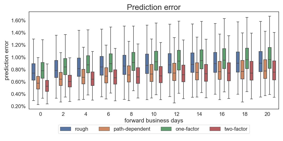
Both graphs show that the dynamical evolution of rough volatility model is far less consistent with market data than its path-dependent and Markovian-counterparts. This further highlights the rigid structural issues associated with rough volatility models.
5.2 Spurious Roughness
We now use the same methodology in [33] to estimate the statistical roughness of the instantaneous volatility process via its proxy, the realized volatility process of all Bergomi models, as instantaneous volatility is unobservable in practice. First, we simulate the trajectories of the instantaneous volatility and under each model, with time step size of 5 minutes for years. Next, we compute the estimated daily via the following:
| (5.1) |
with and then calculate the empirical q-variation of the form:
for different values of and timescale . To remain as close as possible to the experiments performed in [33], we choose and timescale Days. By fixing , we compute the empirical -variation and then use linear regression on ( to estimate its slope . Next, we plot and the slope of the graph is the estimated Hurst index of the simulated process RV.
To simulate instantaneous volatility , we use the calibrated parameters of each model for the implied volatility surface on the day 23 October 2017, calibrated for maturities up to three months with the same seed. For this date, the calibrated parameters for the models are:
Model Calibrated parameters rough path-dependent one-factor two-factor


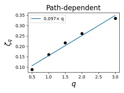

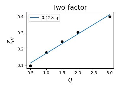


From Figure 14 and 15, we see that the estimate for the Hurst index of the rough Bergomi model is comparing to the calibrated value of for the instantaneous volatility. For the other models, the estimated Hurst index of returns a value between 0.097 to 0.159, comparing to the theoretical Hurst index of 0.5 of their instantaneous volatility. Figure 16 shows the estimated of the actual S&P500 realized volatility over a ten year period between 2007 to 2017, with data coming from the Oxford-Man Institute of Quantitative Finance Realized Library for comparison.
The sample paths of realized volatility used for the estimation of in Figure 14 and 15 of each Bergomi model are included in Appendix C alongside with the annualized realized volatility time series of the S&P500. These sample paths all seem to have an erratic and spiky behavior. Combined with the small estimated statistical , this suggests that the rougher appearance of the realized volatility process does not mean that the underlying process has to be rough, and the estimation of is not enough to discriminate between models, since all of our non-rough models produce similar spurious roughness on any realistic timescales, in line with [1, 19, 39, 49].
Appendix A Sample fits of SPX smile: one week to three months
July 03, 2013


October 23, 2017


Appendix B Sample fits of SPX smile: one week to three years
July 03, 2013


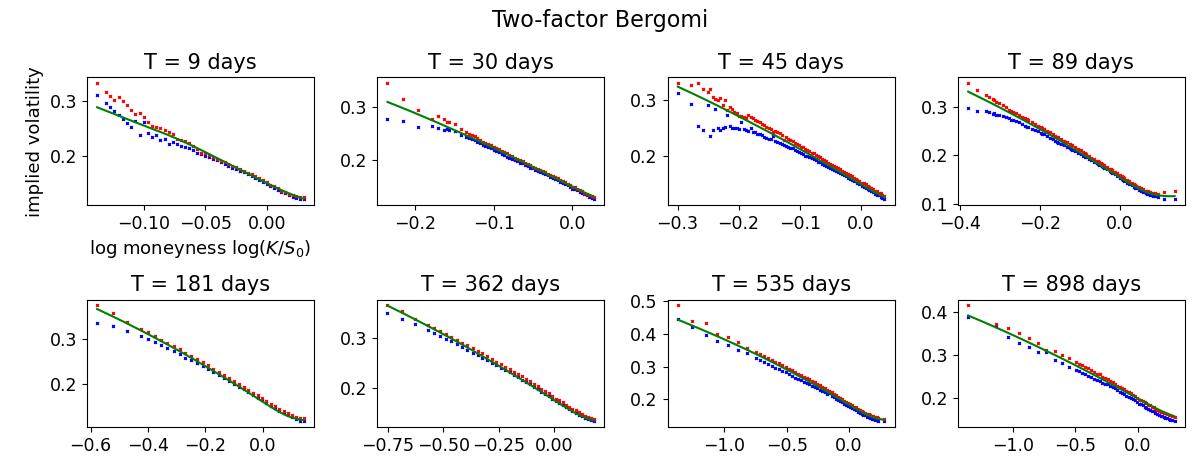
October 23, 2017


Appendix C Simulated realized volatility
Figure 27 shows the simulated trajectories of the realized volatility process under each Bergomi model with the same seed, using the calibrated parameters from Table 5 based on the implied volatility surface on 27 October 2017, and the annualized realized volatility time series of S&P 500 between 2007 to 2017 with data coming from the Oxford-Man Institute’s Realized Library.


References
- Abi Jaber [2019] Eduardo Abi Jaber. Lifting the Heston model. Quantitative Finance, 19(12):1995–2013, 2019.
- Abi Jaber and De Carvalho [2023] Eduardo Abi Jaber and Nathan De Carvalho. Reconciling rough volatility with jumps. Available at SSRN 4387574, 2023.
- Abi Jaber and El Euch [2019] Eduardo Abi Jaber and Omar El Euch. Markovian structure of the Volterra Heston model. Statistics & Probability Letters, 149:63–72, 2019.
- Abi Jaber et al. [2019] Eduardo Abi Jaber, Martin Larsson, and Sergio Pulido. Affine Volterra processes. The Annals of Applied Probability, 29(5):3155–3200, 2019.
- Abi Jaber et al. [2021a] Eduardo Abi Jaber, Christa Cuchiero, Martin Larsson, and Sergio Pulido. A weak solution theory for stochastic volterra equations of convolution type. The Annals of Applied Probability, 31(6):2924–2952, 2021a.
- Abi Jaber et al. [2021b] Eduardo Abi Jaber, Enzo Miller, and Huyên Pham. Linear-quadratic control for a class of stochastic volterra equations: solvability and approximation. The Annals of Applied Probability, 31(5):2244–2274, 2021b.
- Abi Jaber et al. [2022] Eduardo Abi Jaber, Camille Illand, and Shaun Xiaoyuan Li. Joint SPX–VIX calibration with gaussian polynomial volatility models: deep pricing with quantization hints. Available at SSRN 4292544, 2022.
- Abi Jaber et al. [2023] Eduardo Abi Jaber, Camille Illand, and Shaun Li. The quintic ornstein-uhlenbeck volatility model that jointly calibrates spx & vix smiles. Risk Magazine, Cutting Edge Section, 2023.
- Alos et al. [2007] Elisa Alos, Jorge A León, and Josep Vives. On the short-time behavior of the implied volatility for jump-diffusion models with stochastic volatility. Finance and stochastics, 11(4):571–589, 2007.
- Bayer et al. [2016] Christian Bayer, Peter Friz, and Jim Gatheral. Pricing under rough volatility. Quantitative Finance, 16(6):887–904, 2016.
- Bayer et al. [2020] Christian Bayer, Peter K Friz, Paul Gassiat, Jorg Martin, and Benjamin Stemper. A regularity structure for rough volatility. Mathematical Finance, 30(3):782–832, 2020.
- Bergomi [2005] L Bergomi. Smile dynamics II. Risk Magazine, 2005.
- Bergomi [2015] Lorenzo Bergomi. Stochastic volatility modeling. CRC press, 2015.
- Bergomi and Guyon [2012] Lorenzo Bergomi and Julien Guyon. Stochastic volatility’s orderly smiles. Risk, 25(5):60, 2012.
- Bonesini et al. [2023] Ofelia Bonesini, Antoine Jacquier, and Alexandre Pannier. Rough volatility, path-dependent pdes and weak rates of convergence. arXiv preprint arXiv:2304.03042, 2023.
- Carr and Madan [2001] Peter Carr and Dilip Madan. Towards a theory of volatility trading. Option Pricing, Interest Rates and Risk Management, Handbooks in Mathematical Finance, 22(7):458–476, 2001.
- Carr and Wu [2003] Peter Carr and Liuren Wu. What type of process underlies options? a simple robust test. The Journal of Finance, 58(6):2581–2610, 2003.
- Comte and Renault [1998] Fabienne Comte and Eric Renault. Long memory in continuous-time stochastic volatility models. Mathematical finance, 8(4):291–323, 1998.
- Cont and Das [2022] Rama Cont and Purba Das. Rough volatility: fact or artefact? arXiv preprint arXiv:2203.13820, 2022.
- Corlay et al. [2014] Sylvain Corlay, Joachim Lebovits, and Jacques Lévy Véhel. Multifractional stochastic volatility models. Mathematical Finance, 24(2):364–402, 2014.
- Cuchiero and Teichmann [2020] Christa Cuchiero and Josef Teichmann. Generalized feller processes and markovian lifts of stochastic volterra processes: the affine case. Journal of evolution equations, 20(4):1301–1348, 2020.
- Delemotte et al. [2023] Jules Delemotte, Stefano De Marco, and Florent Segonne. Yet another analysis of the sp500 at-the-money skew: Crossover of different power-law behaviours. Available at SSRN 4428407, 2023.
- Ding et al. [1993] Zhuanxin Ding, Clive WJ Granger, and Robert F Engle. A long memory property of stock market returns and a new model. Journal of empirical finance, 1(1):83–106, 1993.
- Dupire [1992] Bruno Dupire. Arbitrage pricing with stochastic volatility. Société Générale, 1992.
- Forde et al. [2020] Martin Forde, Masaaki Fukasawa, Stefan Gerhold, and Benjamin Smith. The rough bergomi model as h→ 0–skew flattening/blow up and non-gaussian rough volatility. preprint, 2020.
- Fouque et al. [2000] Jean-Pierre Fouque, George Papanicolaou, and K Ronnie Sircar. Derivatives in financial markets with stochastic volatility. Cambridge University Press, 2000.
- Fouque et al. [2003] Jean-Pierre Fouque, George Papanicolaou, Ronnie Sircar, and Knut Solna. Multiscale stochastic volatility asymptotics. Multiscale Modeling & Simulation, 2(1):22–42, 2003.
- Fouque et al. [2004] Jean-Pierre Fouque, George Papanicolaou, Ronnie Sircar, and Knut Solna. Maturity cycles in implied volatility. Finance and Stochastics, 8:451–477, 2004.
- Friz et al. [2022] Peter K Friz, Jim Gatheral, and Radoš Radoičić. Forests, cumulants, martingales. The Annals of Probability, 50(4):1418–1445, 2022.
- Fukasawa [2011] Masaaki Fukasawa. Asymptotic analysis for stochastic volatility: martingale expansion. Finance and Stochastics, 15:635–654, 2011.
- Fukasawa [2021] Masaaki Fukasawa. Volatility has to be rough. Quantitative Finance, 21(1):1–8, 2021.
- Gatheral [2008] Jim Gatheral. Consistent modeling of spx and vix options. In Bachelier congress, volume 37, pages 39–51, 2008.
- Gatheral et al. [2018] Jim Gatheral, Thibault Jaisson, and Mathieu Rosenbaum. Volatility is rough. Quantitative finance, 18(6):933–949, 2018.
- Gulisashvili [2018] Archil Gulisashvili. Large deviation principle for volterra type fractional stochastic volatility models. SIAM Journal on Financial Mathematics, 9(3):1102–1136, 2018.
- Guyon [2021] Julien Guyon. The smile of stochastic volatility: Revisiting the bergomi-guyon expansion. Available at SSRN 3956786, 2021.
- Guyon [2022a] Julien Guyon. Dispersion-constrained martingale schrödinger bridges: Joint entropic calibration of stochastic volatility models to s&p 500 and vix smiles. Available at SSRN 4165057, 2022a.
- Guyon [2022b] Julien Guyon. The vix future in bergomi models: Fast approximation formulas and joint calibration with s&p 500 skew. SIAM Journal on Financial Mathematics, 13(4):1418–1485, 2022b.
- Guyon and El Amrani [2022] Julien Guyon and Mehdi El Amrani. Does the term-structure of equity at-the-money skew really follow a power law? Available at SSRN 4174538, 2022.
- Guyon and Lekeufack [2022] Julien Guyon and Jordan Lekeufack. Volatility is (mostly) path-dependent. Volatility Is (Mostly) Path-Dependent (July 27, 2022), 2022.
- Harms and Stefanovits [2019] Philipp Harms and David Stefanovits. Affine representations of fractional processes with applications in mathematical finance. Stochastic Processes and their Applications, 129(4):1185–1228, 2019.
- Horvath et al. [2017] Blanka Horvath, Antoine Jacquier, and Aitor Muguruza. Functional central limit theorems for rough volatility. arXiv preprint arXiv:1711.03078, 2017.
- Horvath et al. [2021] Blanka Horvath, Aitor Muguruza, and Mehdi Tomas. Deep learning volatility: a deep neural network perspective on pricing and calibration in (rough) volatility models. Quantitative Finance, 21(1):11–27, 2021.
- Jacquier and Pannier [2022] Antoine Jacquier and Alexandre Pannier. Large and moderate deviations for stochastic volterra systems. Stochastic Processes and their Applications, 149:142–187, 2022.
- Jaisson and Rosenbaum [2016] Thibault Jaisson and Mathieu Rosenbaum. Rough fractional diffusions as scaling limits of nearly unstable heavy tailed hawkes processes. The Annals of Applied Probability, 26(5):2860–2882, 2016. ISSN 10505164.
- Liu et al. [1997] Yanhui Liu, Pierre Cizeau, Martin Meyer, C-K Peng, and H Eugene Stanley. Correlations in economic time series. Physica A: Statistical Mechanics and its Applications, 245(3-4):437–440, 1997.
- Mechkov [2015] Serguei Mechkov. Fast-reversion limit of the Heston model. Available at SSRN 2418631, 2015.
- Muzy et al. [2000] Jean-François Muzy, Jean Delour, and Emmanuel Bacry. Modelling fluctuations of financial time series: from cascade process to stochastic volatility model. The European Physical Journal B-Condensed Matter and Complex Systems, 17:537–548, 2000.
- Perelló et al. [2004] Josep Perelló, Jaume Masoliver, and Jean-Philippe Bouchaud. Multiple time scales in volatility and leverage correlations: a stochastic volatility model. Applied Mathematical Finance, 11(1):27–50, 2004.
- Rogers [2019] L Rogers. Things we think we know, 2019.
- Rømer [2022] Sigurd Emil Rømer. Empirical analysis of rough and classical stochastic volatility models to the spx and vix markets. Quantitative Finance, 22(10):1805–1838, 2022.
- Viens and Zhang [2019] Frederi Viens and Jianfeng Zhang. A martingale approach for fractional brownian motions and related path dependent pdes. The Annals of Applied Probability, 29(6):3489–3540, 2019.