Vocabulary-informed Zero-shot and Open-set Learning
Abstract
Despite significant progress in object categorization, in recent years, a number of important challenges remain; mainly, the ability to learn from limited labeled data and to recognize object classes within large, potentially open, set of labels. Zero-shot learning is one way of addressing these challenges, but it has only been shown to work with limited sized class vocabularies and typically requires separation between supervised and unsupervised classes, allowing former to inform the latter but not vice versa. We propose the notion of vocabulary-informed learning to alleviate the above mentioned challenges and address problems of supervised, zero-shot, generalized zero-shot and open set recognition using a unified framework. Specifically, we propose a weighted maximum margin framework for semantic manifold-based recognition that incorporates distance constraints from (both supervised and unsupervised) vocabulary atoms. Distance constraints ensure that labeled samples are projected closer to their correct prototypes, in the embedding space, than to others. We illustrate that resulting model shows improvements in supervised, zero-shot, generalized zero-shot, and large open set recognition, with up to 310K class vocabulary on Animal with Attributes and ImageNet datasets.
Index Terms:
Vocabulary-informed learning, Generalized zero-shot learning, Open-set recognition, Zero-shot learning.1 Introduction
Object recognition, more specifically object categorization, has seen unprecedented advances in recent years with development of convolutional neural networks (CNNs) [41]. However, most successful recognition models, to date, are formulated as supervised learning problems, in many cases requiring hundreds, if not thousands, labeled instances to learn a given concept class [15]. This exuberant need for large labeled instances has limited recognition models to domains with hundreds to thousands of classes. Humans, on the other hand, are able to distinguish beyond basic level categories [8]. Even more impressive is the fact that humans can learn from few examples, by effectively leveraging information from other object category classes, and even recognize objects without ever seeing them (e.g., by reading about them on the Internet). This ability has spawned the research in few-shot and zero-shot learning.
Zero-shot learning (ZSL) has now been widely studied in a variety of research areas including neural decoding of fMRI images [54], character recognition [44], face verification [42], object recognition [43], and video understanding [27, 82]. Typically, zero-shot learning approaches aim to recognize instances from the unseen or unknown testing target categories by transferring information through intermediate-level semantic representations, from known observed source (or auxiliary) categories for which many labeled instances exist. In other words, supervised classes/instances, are used as context for recognition of classes that contain no visual instances at training time, but that can be put in some correspondence with supervised classes/instances. Therefore, a general experimental setting of ZSL is that the classes in target and source (auxiliary) dataset are disjoint. Typically, the learning is done on the source dataset and then information is transferred to the target dataset, with performance measured on the latter.
This setting has a few important drawbacks: (1) it assumes that target classes cannot be mis-classified as source classes and vice versa; this greatly and unrealistically simplifies the problem; (2) the target label set is often relatively small, between ten [43] and several thousand unknown labels [24], compared to at least entry level categories that humans can distinguish; (3) large amounts of data in the source (auxiliary) classes are required, which is problematic as it has been shown that most object classes have very few instances (long-tailed distribution of objects in the world [72]); and (4) the vast open set vocabulary and corresponding semantic knowledge, defined as part of ZSL [54], is not leveraged in any way to inform the learning or source class recognition.

A few works recently looked at resolving (1) through class-incremental learning [66, 68] or generalized zero-shot learning (G-ZSL) [11, 54] which are designed to distinguish between seen (source) and unseen (target) classes at the testing time and apply an appropriate model – supervised for the former and ZSL for the latter. However, (2)–(4) remain largely unresolved. In particular, while (2) and (3) are artifacts of the ZSL setting, (4) is more fundamental; e.g., a recent study [34] argues that concepts, in our own brains, are represented in the form of a continuous semantic space mapped smoothly across the cortical surface. For example, consider learning about a car by looking at image instances in Figure 1. Not knowing that other motor vehicles exist in the world, one may be tempted to call anything that has 4-wheels a car. As a result, the zero-shot class truck may have a large overlap with the car class (see Figure 1 (left)). However, imagine knowing that there also exist many other motor vehicles (trucks, mini-vans, etc). Even without having visually seen such objects, the very basic knowledge that they exist in the world and are closely related to a car should, in principle, alter the criterion for recognizing instance as a car (making the recognition criterion stricter in this case). Encoding this in our vocabulary-informed learning model results in better separation among classes (see Figure 1 (right)).
To tackle the limitations of ZSL and towards the goal of generic recognition, we propose the idea of vocabulary-informed learning. Specifically, assuming we have few labeled training instances and a large, potentially open set, vocabulary/semantic dictionary (along with textual sources from which statistical semantic relations among vocabulary atoms can be learned), the task of vocabulary-informed learning is to learn a unified model that utilizes this semantic dictionary to help train better classifiers for observed (source) classes and unobserved (target) classes in supervised, zero-shot, generalized zero-shot, and open set image recognition settings.
In particular, we formulate Weighted Maximum Margin Vocabulary-informed Embedding (WMM-Voc), which learns a joint embedding for visual features and semantic words. In this formulation, two maximum margin sets of constraints are simultaneously optimized. The first set ensures that labeled training visual instances, belonging to a particular class, project close to semantic word vector prototype corresponding to the class name in the embedding space. The second set ensures that these instances are closer to the correct class word vector prototype than to any of the incorrect ones in the embedding space; including those that may not contain training data (i.e., zero-shot). The constraints in the first set further take into the account the distribution of training samples for each class, and nearby classes, to dynamically set appropriate margins. In other words, for some classes the distance, between the projected training sample and the word vector prototype, is explicitly penalized more (or less) than for others. This weighting is derived using extreme values theory.
Contributions: Our main contribution is to propose a novel paradigm for potentially open set image recognition: vocabulary-informed learning (Voc), which is capable of utilizing vocabulary over unsupervised items, during training, to improve recognition. We extend the model initially proposed by us in a conference paper [29] to include class-specific weighting in the data term, as well as the ability to run the models as an end-to-end network. Particularly, classification is done through the nearest-neighbor distance to class prototypes in the semantic embedding space. Semantic embedding is learned subject to constraints ensuring that labeled images project into semantic space such that they end up closer to the correct class prototypes than to incorrect ones (whether those prototypes are part of the source or target classes). We show that word embedding (word2vec) can be used effectively to initialize the semantic space. Experimentally, we illustrate that through this paradigm: we can achieve very competitive supervised (on source classes), ZSL (on target classes) and G-ZSL performance, as well as open set image recognition performance with a large number of unobserved vocabulary entities (up to ); effective learning with few samples is also illustrated. Critically, our models can be directly utilized in G-ZSL scenario and still has much better results than the baselines.
2 Related Work
Our model belongs to a class of transfer learning approaches [55], also sometimes called meta-learning [79] or learning to learn [70]. The key idea of transfer learning is to transfer the knowledge from previously learned categories to recognize new categories with no training examples (zero-shot learning [43, 59]), few examples (one-shot learning [71, 19]) or from vast open set vocabulary [29]. The process of knowledge transfer can be done by sharing features [5, 33, 22, 4, 81, 73], semantic attributes [43, 58, 60], or contextual information [74].
Visual-semantic embeddings have been widely used for transfer learning. Such models embed visual features into a semantic space by learning projections of different forms. Examples include WSABIE [80], ALE [2], SJE [3], DeViSE [24], SVR [18, 43], kernel embedding [33] and Siamese networks [37].
2.1 Open-set Recognition
The term “open set recognition” was initially defined in [65, 66] and formalized in [6, 63, 7] which mainly aim at identifying whether an image belongs to a seen or unseen classes. The problem is also known as class-incremental learning. However, none of these methods can further identify classes for unseen instances. The exceptions are [53, 24] which augment zero-shot (unseen) class labels with source (seen) labels in some of their experimental settings. Similarly, we define the open set image recognition as the problems of recognizing the class name of an image from a potentially very large open set vocabulary (including, but not limited to source and target labels). Note that methods like [65, 66] are orthogonal but potentially useful here – it is still worth identifying seen or unseen instances to be recognized with different label sets. Conceptually similar, but different in formulation and task, open-vocabulary object retrieval [32] focused on retrieving objects using natural language open-vocabulary queries.
2.2 One-shot Learning
While most of machine learning-based object recognition algorithms require a large amount of training data, one-shot learning [20] aims to learn object classifiers from one, or very few examples. To compensate for the lack of training instances and enable one-shot learning, knowledge must be transferred from other sources, for example, by sharing features [5], semantic attributes [27, 43, 58, 60], or contextual information [74]. However, none of the previous work had used the open set vocabulary to help learn the object classifiers.
2.3 Zero-shot Learning
Zero-shot Learning (ZSL) aims to recognize novel classes with no training instance by transferring knowledge from source classes. ZSL was first explored with use of attribute-based semantic representations [18, 26, 27, 28, 42, 56]. This required pre-defined attribute vector prototypes for each class, which is costly to obtain for a large-scale dataset. Recently, semantic word vectors were proposed as a way to embed any class name without human annotation effort; they can therefore serve as an alternative semantic representation [3, 24, 31, 53] for ZSL. Semantic word vectors are learned from large-scale text corpus by language models, such as word2vec [52] or GloVec [57]. However, most of the previous work only use word vectors as semantic representations in ZSL setting, but have neither (1) utilized semantic word vectors explicitly for learning better classifiers; nor (2) for extending ZSL setting towards open set image recognition. A notable exception is [53] which aims to recognize 21K zero-shot classes given a modest vocabulary of 1K source classes; we explore vocabularies that are up to an order of the magnitude larger – 310K.
Generalized zero-shot recognition (G-ZSL) [11] relaxed the problem setup of conventional zero-shot learning by considering the training classes in the recognition step. Chao et al. [11] investigated the G-ZSL task and found that it is less effective to directly extend the existing zero-shot learning algorithms to deal with G-ZSL setting. Recently, Xian et al. [54] systematically compared the evaluation settings for ZSL and G-ZSL. Comparing against existing ZSL models, which are inferior in the G-ZSL scenario, we show that our vocabulary-informed frameworks can be directly utilized for G-ZSL and achieve very competitive performance.
2.4 Visual-semantic Embedding
Mapping between visual features and semantic entities has been explored in three ways: (1) directly learning the embedding by regressing from visual features to the semantic space using Support Vector Regressors (SVR) [18, 43] or neural network [68]; (2) projecting visual features and semantic entities into a common new space, such as SJE [3], WSABIE [80], ALE [2], DeViSE [24], and CCA [25, 28]; (3) learning the embeddings by regressing from the semantic space to visual features, including [38, 1, 49, 10].
In contrast to other embedding methods, our model trains a better visual-semantic embedding from only few training instances with the help of a large amount of open set vocabulary items (using a maximum margin strategy). Our formulation is inspired by the unified semantic embedding model of [35], however, unlike [35], our formulation is built on word vector representation, contains a data term, and incorporates constraints to unlabeled vocabulary prototypes.
3 Vocabulary-informed Learning
3.1 Problem setup
Assume a labeled source dataset of samples, where is the image feature representation of image and is a class label taken from a set of English words or phrases ; consequently, is the number of source classes. Further, suppose another set of class labels for target classes , also taken from , such that , for which no labeled samples are available. We note that potentially .
Given a new test image feature vector the goal is then to learn a function , using all available information, that predicts a class label . Note that the form of the problem changes drastically depending on the label set assumed for :
-
•
Supervised learning: ;
-
•
Zero-shot learning: ;
-
•
Generalized zero-shot learning: ;
-
•
Open set recognition: .
Note that open set recognition is similar to generalized zero-shot learning, however, in open set setting additional distractor classes that do not exist in either source or target datasets are present. We posit that a single unified can be learned for all cases. We formalize the definition of vocabulary-informed learning (Voc) as follows:
Definition 3.1.
Vocabulary-informed Learning (Voc): is a learning setting that makes use of complete vocabulary data () during training. Unlike a more traditional ZSL that typically makes use of the vocabulary (e.g., semantic embedding) at test time, Voc utilizes exactly the same data during training. Notably, Voc requires no additional annotations or semantic knowledge; it simply shifts the burden from testing to training, leveraging the vocabulary to learn a better model.
The vocabulary can be represented by semantic embedding space learned by word2vec [52] or GloVec [57] on large-scale corpus; each vocabulary entity is represented as a distributed semantic vector . Semantics of embedding space help with knowledge transfer among classes, and allow ZSL, G-ZSL and open set image recognition. Note that such semantic embedding spaces are equivalent to the “semantic knowledge base” for ZSL defined in [54] and hence make it appropriate to use Vocabulary-informed Learning in ZSL.
3.2 Learning Embedding and Recognition
Assuming we can learn a mapping , from image features to this semantic space, recognition can be carried out using simple nearest neighbor distance, e.g., if is closer to than to any other word vector; in this context can be interpreted as the prototype of the class . Essentially, the attribute or semantic word vector of the class name can be taken as the class prototype [30]. The core question is then how to learn the mapping and what form of inference is optimal in the semantic space. For learning we propose the discriminative maximum margin criterion that ensures that labeled samples project closer to their corresponding class prototypes than to any other prototype in the open set vocabulary .
Learning Embedding: To learn the function , one needs to establish the correspondence between visual feature space and semantic space. Particularly, in the training step, each image sample is regressed towards its corresponding class prototype by minimizing
| (1) |
where ; and is the mapping from image features to semantic space; indicates the Frobenius Norm. If is a linear mapping, we have the closed form solution for Eq. (1). The loss function in Eq. (1) can be interperted as a variant of SVR embedding. However, this is too limiting. To learn the linear embedding matrix , we introduce and discuss two sets of methods in Section 3.3 and Section 3.4.
Recognition: The recognition step can be formulated using the nearest neighbor classifier. Given a testing instance ,
| (2) |
Eq. (2) measures the distance between predicted vector and the class prototypes in the semantic space. In terms of different label set, we can do supervise, zero-shot, generalized zero-shot or open set recognition without modifications.
In particular, we explore a simple variant of Eq. (2) to classify the testing instance ,
| (3) |
where the Nearest Neighbor (NN) classifier measures distance between the predicted semantic vectors and a function of prototypes in the semantic space, e.g., is equivalent to Eq (2). In practice, we employ semantic vector prototype averaging to define . For example, sometimes, there might be more than one positive prototype, such as pig, pigs and hog. In such the circumstance, choosing the most likely prototype and using NN may not be sensible, hance we introduce the averaging strategy to consider more prototypes for robustness. Note that this strategy is known as Rocchio algorithm in information retrieval. Rocchio algorithm is a method for relevance feedback that uses more relevant instances to update the query for better recall and possibly precision in the vector space (Chap 14 in [51]). It was first suggested for use in ZSL in [27]; more sophisticated algorithms [25, 58] are also possible.
3.3 Maximum Margin Voc Embedding (MM-Voc)
The maximum margin vocabulary-informed embedding learns the mapping , from low-level features to the semantic word space by utilizing maximum margin strategy. Specifically, consider , where111Generalizing to a kernel version is straightforward, see [76]. . Ideally we want to estimate such that for all labeled instances in . Note that we would obviously want this to hold for instances belonging to unobserved classes as well, but we cannot enforce this explicitly in the optimization as we have no labeled samples for them.
Data Term: The easiest way to enforce the above objective is to minimize Euclidian distance between sample projections and appropriate prototypes in the embedding space,
| (4) |
Where we need to minimize this term with respect to each instance , where is the class label of in . Such embedding is also known, in the literature, as data embedding [35] or compatibility function [3].
To make the embedding more comparable to support vector regression (SVR), we employ the maximal margin strategy – insensitive smooth SVR (SSVR) [46] in Eq. (1). That is,
| (5) |
where ; is regularization coefficient.
| (6) |
; indicates the -th value of corresponding vector; is the -th column of , and is the scaling weight derived from the density of class and it’s neighboring classes. In our conference version [29], equal weight is used for all classes. Here we notice that it is beneficial to use the density/coverage of each labeled training class as the constraint in learning the projection from visual feature space to semantic space. We introduce a specific weighting strategy to compute in Section 3.4.
The conventional SVR is formulated as a constrained minimization problem, i.e., convex quadratic programming problem, while SSVR employs quadratic smoothing [89] to make Eq. (5) differentiable everywhere, and thus SSVR can be solved as an unconstrained minimization problem directly222In practice, our tentative experiments shows that the Eq. (4) and Eq. (5) will lead to the similar results, on average; but formulation in Eq. (5) is more stable and has lower variance. .
Triplet Term: Data term above only ensures that labelled samples project close to their correct prototypes. However, since it is doing so for many samples and over a number of classes, it is unlikely that all the data constraints can be satisfied exactly. Specifically, consider the following case, if is in the part of the semantic space where no other entities live (i.e., distance from to any other prototype in the embedding space is large), then projecting further away from is asymptomatic, i.e., will not result in misclassification. However, if the is close to other prototypes then minor error in regression may result in misclassification.
To embed this intuition into our learning, we enforce more discriminative constraints in the learned semantic embedding space. Specifically, the distance of should not only be as small as possible, but should also be smaller than the distance , . Formally, we define the triplet term
| (7) |
where (or more precisely ) is selected from the open vocabulary; is the margin gap constant. Here, indicates the quadratically smooth hinge loss [89] which is convex and has the gradient at every point. To speedup computation, we use the closest target prototypes to each source/auxiliary prototype in the semantic space. We also define similar constraints for the source prototype pairs:
| (8) |
where is selected from source/auxiliary dataset vocabulary. This term enforces that should be smaller than the distance , . To facilitate the computation, we similarly use closest prototypes that are closest to each prototype in the source classes. Note that, the Crammer and Singer loss [75, 13] is the upper bound of Eq. (7) and (8) which we use to tolerate slight variants of (e.g., the prototypes of ’pigs’ Vs. ’pig’).
To sum up, the complete triplet maximum margin term is:
| (9) |
We note that the form of rank hinge loss in Eq. (7) and (8) is similar to DeViSE [24], but DeViSE only considers loss with respect to source/auxiliary data and prototypes.
Maximum Margin Vocabulary-informed Embedding: The complete combined objective can now be written as:
| (10) |
where is the coefficient that controls contribution of the two terms. One practical advantage is that the objective function in Eq. (10) is an unconstrained minimization problem which is differentiable and can be solved with L-BFGS. is initialized with all zeros and converges in iterations.
3.4 Weighted Maximum Margin Voc Embedding (WMM-Voc)

We note that there is no previous method that directly estimates the density of source training classes in the semantic space. However, doing so may lead to several benefits. First, the number of training instances in source classes may be unbalanced. In such a case, an estimate of the density of samples in a training class can be utilized as a constraint in learning the embedding characterized by Eq. (6). Second, in the semantic space, the instances from the classes whose data samples span a large radius [62] may reside in the neighborhood of many other classes or open vocabulary. This can happen when the embedding is not well learned. We can interpret this phenomenon as hubness [67, 45]333However, the causes for hubness are still under investigation [16, 67].. Adding a penalty based on the density of each training class may be helpful in better learning the embedding and alleviating the hubness problem.
This subsection introduces a strategy for estimating the density of each known class in the semantic space (i.e., in Eq. (6)). Generally, we know the prototype of each known and novel class in the semantic space. To estimate the density/coverage of a known class, one needs to look at pairwise distance between a prototype and the nearest negative instance and the furthest positive instance. This intuition leads us to introduce the concept of margin distribution.
Margin Distribution: The concept of margin is fundamental to maximum margin classifiers (e.g., SVMs) in machine learning. The margin enables an intuitive interpretation of such classifiers in searching for the maximum margin separator in a Reproducing Kernel Hilbert Space. Previous margin classifiers [92] aim to maximize a single margin across all training instances. In contrast, some recent studies [90, 62, 64, 17] suggest that the knowledge of margin distribution of instances, rather than a single margin across all instances, is crucial for improving the generalization performance of a classifier.
The “instance margin” is defined as the distance between one instance and the separating hyperplane. Formally, for one instance in the semantic space and sufficiently many444In our experiments, we use all available training instances here. samples () drawn from well behaved class distributions555The well behaved indicates that the moments of the distribution should be well-defined. For example, Cauchy distribution is not well-behaved [39].. We define the distance . For instance , we can obtain a set of distances with the minimal values . As shown in [62], the distribution for the minimal values of the margin distance is characterized by a Weibull distribution. Based on this finding, we can express the probability of being included in the boundary estimated by :
| (11) |
where and are Weibull shape and scale parameters obtained by fitting using Maximum Likelihood Estimate (MLE), which is summarized666codes released in https://github.com/xiaomeiyy/WMM-Voc. in Alg. 1. Equation (11) quantitatively describes the margin of one specific class, probabilistically, in our semantic embedding space. Note that Eq. (11) requires to be non-degenerate margin distribution, which is essentially guaranteed by Extreme Value Theorem [40].
Input: Extreme values
Output: Estimated parameters
If :
.
Else:
1. Sort to get
(where is the re-ordered value).
2. Maximum likelihood estimator for :
| (12) |
3. Solve Eq. (12), and numerically estimate .
(e.g., using fzero function in MATLAB)
4. Compute .
Margin Distribution of Prototypes: Consider a class which in the embedding space is represented by a prototype . In accordance with above formalism, we can also assume sufficiently many samples drawn from other () well behaved class distributions. We can also consider the prototypes of vast open vocabulary (, ). Under these assumptions, we can obtain a set of distances for the prototype . As a result, the distribution for the minimal values of the margin distance for is given by a Weibull distribution. The probability that is included in the boundary estimated by is given by
| (13) |
The above equation models the distribution of minimum value; thus it can be used to estimate the boundary density (or more specifically, the boundary distribution) of class .
We set significant level to 0.05 to approximately estimate the minimal value . As illustrated in Figure 2, if we will assume does not belong to the prototype ; otherwise, is included in the boundary estimated by . In term of the significant level of 0.05, we can further denote the minimal values as , i.e., . Thus we have
| (14) |
Coverage Distribution of Prototypes: Now, for class consider the nearest instance from another class where ; with sufficient many instances from class , we have pairwise unique ("within class") distance:
| (15) |
We consider outliers those instances that have larger distance to than the nearest instance () of another class. To remove the outliers we hence consider . As illustrated in Figure 2, we only consider positive instances within the orange circle and all other instances with larger distance are removed. Then the distribution of the largest distance will follow a reversed Weibull distribution. This allows us to get the probability distribution to describe positive instances,
| (16) |
where and are reverse Weibull shape and scale parameters individually obtained from fitting the largest , is the distance between instance and prototype, is the probability that the instance is in the class.
Similar to the margin distribution, we can estimate the coverage by setting the significant level to . As shown in Figure 2, we establish two boundaries to estimate the scale of each class probabilistically. If , is included in the coverage distribution . The maximum values can be computed as . It results in,
| (17) |
By combining the terms computed in Eq. (14) and (17), we can obtain the weight for class in Eq. (6),
| (18) |
As explained in Algorithm 1, we set in one-shot setting. In few-shot learning setting, we can estimate and directly. In addition, such an initialization of weights ( and ) intrinsically helps learn the embedding weight .
The learning process of parameters: The process could be interpreted as a form of block coordinate descent where we estimate the embedding/mapping; then density within that embedding and so on. In practice, the weights are initially randomized. But they do not play an important role at the beginning of the optimization, since is very large in the first few iterations. In other words, the optimization is initially dominated by the data term and maximum margin terms play little role. However, once we can get a relative good mapping (i.e., smaller ) after several training iterations, the weight starts becoming significant. By virtue of such an optimization, the weighted version can achieve better performance than the previous non-weighted version in our conference paper [29].
Deep Weighted Maximum Margin Voc Embedding (Deep WMM-Voc). In practice, we extend WMM-Voc to include a deep network for feature extraction. Rather than extracting low-level features using an off-the-shelf pre-trained model in Eq. (10), we use an integrated deep network to extract from the raw images. As a result, the loss function in Eq. (10) is also used to optimize the parameters of the deep network. In particular, we fix the convolutional layers of corresponding network and fine-tune the last fully connected layer in our task. The network was trained using stochastic gradient descendent.
4 Experiments
4.1 Experimental setup
We conduct our experiments on Animals with Attributes (AwA) dataset, and ImageNet / dataset.
AwA dataset: AwA consists of 50 classes of animals ( images in total). In [43] standard split into 40 source/auxiliary classes () and 10 target/test classes () is introduced. We follow this split for supervised and zero-shot learning. We use ResNet101 features (downloaded from [54]) on AwA to make the results more easily comparable to state-of-the-art.
ImageNet / dataset: ImageNet is a large-scale dataset. We use () classes of ILSVRC as the source/auxiliary classes and () classes of ILSVRC 2010 that are not used in ILSVRC as target data. We use pre-trained VGG-19 model [12] to extract deep features for ImageNet.
Recognition tasks: We consider several different settings in a variety of experiments. We first divide the two datasets into source and target splits. On source classes, we can validate whether our framework can be used to solve one-shot and supervised recognition. By using both the source and target classes, transfer learning based settings can be evaluated.
-
1.
Supervised recognition: learning is on source classes; test instances come from the same classes with as recognition vocabulary. In particular, under this setting, we also validate the one- and few-shot recognition scenarios, i.e., classes have one or few training examples.
-
2.
Zero-shot recognition: In ZSL, learning is on the source classes with vocabulary; test instances come from target dataset with as recognition vocabulary.
-
3.
General-zero-shot recognition: G-ZSL uses source classes to learn, with test instances coming from either target or original recognition vocabulary.
-
4.
Open-set recognition: Again source classes are used for learning, but the entire open vocabulary with atoms is used at test time. In practice, test images come from both source and target splits (similar to G-ZSL); however, unlike G-ZSL there are additional distractor classes. In other words, chance performance for open-set recognition is much lower than for G-ZSL.
We test both our Voc variants – MM-Voc and WMM-Voc. Additionally, we also validate the Deep WMM-Voc by fine-tuning the WMM-Voc on VGG-19 architecture and optimizing the weights with respect to the loss in Eq. (10).
Competitors: We compare to a variety of the models in the literature, including:
-
1.
SVM: SVM classifier trained directly on the training instances of source data, without the use of semantic embedding. This is the standard (Supervised/One-shot) learning setting and the learned classifier can only predict the labels within the source classes. Hence, SVM is inapplicable in ZSL, G-ZSL, and open-set recognition settings.
-
2.
SVR-Map: SVR is used to learn and the recognition is done, similar to our method, in the resulting semantic manifold. This corresponds to only optimizing Eq. (5).
-
3.
Deep-SVR: This is a variant SVR, which further allows fine-tuning of the underlying neural network generating the features. In this case, is expressed as the last linear layer and the entire network is fine-tuned with respect to the loss encoding only the data term (Eq. (5)).
-
4.
SAE: SAE is a semantic encoder-decoder paradigm that projects visual features into a semantic space and then reconstructs the original visual feature representation [38]. The SAE has two variants in learning the embedding space, i.e., semantic space to feature space (SF), and feature space to semantic space (FS). By default, the best result of these two variants are reported.
-
5.
ESZSL: ESZSL first learns the mapping between visual features and attributes, then models the relationship between attributes and classes [61].
-
6.
DeVise, ConSE, AMP: To compare with state-of-the-art large-scale zero-shot learning approaches we implement DeViSE [24] and ConSE [53]777Codes for [24] and [53] are not publicly available.. ConSE uses a multi-class logistic regression classifier for predicting class probabilities of source instances; and the parameter T (number of top-T nearest embeddings for a given instance) was selected from that gives the best results. ConSE method in supervised setting works the same as SVR. We use the AMP code provided on the author webpage [31].
Metrics: Classification accuracies are reported as the evaluation metrics on most of tasks. In our conference version [29], we further introduce an evaluation setting for Open-set tasks where we do not assume that test data comes from either source/auxiliary domain or target domain. Thus we split the two cases (i.e., Supervised-like, and Zero-shot-like settings), to mimic Supervised and Zero-shot scenarios for easier analysis. Particularly, in G-ZSL task, this newly introduced evaluation setting is corresponding to the evaluation metrics defined in [85]: (1) : Test instances from seen classes, the prediction candidates include both seen and unseen classes; (2) : Test instances from unseen classes, the prediction candidates include both seen and unseen classes. (3) The harmonic mean is used as the main evaluation metric to further combine the results of both and :
| (19) |
Setting of Parameters: For the recognition tasks, we learn classifiers by using various number of training instances. We compare relevant baselines with results of our method variants: MM-Voc, WMM-Voc, Deep WMM-Voc. Each setting is repeated/tested 10 times. The averaged results are reported to reduce the variance. For each setting, our Voc methods are trained by a single model to be capable of solving the tasks of supervised, zero-shot, G-ZSL and open-set recognition. Specifically,
-
1.
In Deep WMM-Voc, we fix to and with the learning rate initially set to and is reduced by every epochs. and are set to in order to balance performance and computational cost of pairwise constraints.
-
2.
To solve Eq. (10) at a scale, one can use Stochastic Gradient Descent (SGD) which makes great progress initially, but often is slow when approaching convergence. In contrast, the L-BFGS method mentioned above can achieve steady convergence at the cost of computing the full objective and gradient at each iteration. L-BFGS can usually achieve better results than SGD with good initialization, however, is computationally expensive. To leverage benefits of both of these methods, we utilize a hybrid method to solve Eq. (10) in large-scale datasets: the solver is initialized with few instances to approximate the gradients using SGD first; then gradually more instances are used and switch to L-BFGS is made with iterations. This solver is motivated by Friedlander et al. [23], who theoretically analyzed and proved the convergence for the hybrid optimization methods. In practice, we use L-BFGS and the Hybrid algorithms for AwA and ImageNet respectively. The hybrid algorithm can save between training time as compared with L-BFGS.
Open set vocabulary. We use Google word2vec to learn the open set vocabulary set from a large text corpus of around billion words: UMBC WebBase ( billion words), the latest Wikipedia articles ( billion words) and other web documents ( billion words). Some rare (low frequency) words and high frequency stopping words were pruned in the vocabulary set: we remove words with the frequency or times. The result is a vocabulary of around 310K words/phrases with , which is defined as [66].
4.2 Experimental results on AwA dataset

| Methods | S. Sp | Features | Acc. |
|---|---|---|---|
| WMM-Voc | W | 90.79 | |
| WMM-Voc: closed | W | 84.51 | |
| Deep WMM-Voc | W | 90.65 | |
| Deep WMM-Voc: closed | W | 83.85 | |
| SAE | W | ||
| ESZSL | W | ||
| Deep-SVR | W | ||
| Akata et al. [3] | A+W | ||
| TMV-BLP [25] | A+W | ||
| AMP (SR+SE) [31] | A+W | ||
| PST[58] | A+W | ||
| Latem [83] | A+W | 74.80 | |
| SJE [3] | A+W | 76.70 | |
| DeViSE [24] | W | 72.90 | |
| ConSE [53] | W | 63.60 | |
| CMT [68] | W | 58.90 | |
| SSE [91] | W | 54.50 | |
| SSE [91] | W | 57.49 | |
| TASTE[87] | W | 89.40 | |
| KLDA+KRR[48] | W | 79.30 | |
| CLN+KRR[48] | W | 81.00 | |
| UVDS[50] | W | 62.88 | |
| DEM[10] | W | 86.70 | |
| DS [60] | W/A | ||
| SYNC [9] | W/A | 72.20 | |
| Relation Net[69] | A | 84.50 | |
| ESZSL [61] | A | 74.70 | |
| UVDS[50] | A | 80.28 | |
| GFZSL[78] | A | 80.50 | |
| DEM[10] | A | 78.80 | |
| SE-GZSL[77] | A | 69.50 | |
| cycle-CLSWGAN[21] | A | 66.30 | |
| f-CLSWGAN[84] | A | 68.20 | |
| PTMCA[47] | A | 66.20 | |
| Jayaraman et al. [36] | A | low-level | |
| DAP [43] | A | ||
| DAP [43] | A | 57.10 | |
| DAP [43] | A | ||
| ALE [2] | A | 78.60 | |
| Yu et al. [86] | A | low-level | |
| IAP [43] | A | ||
| HEX [14] | A | ||
| AHLE [2] | A | low-level |
4.2.1 Learning Classifiers from Few Source Training Instances
| Dimension | SVR-Map | Deep-SVR | SAE | ESZSL | MM-Voc | WMM-Voc | Deep WMM-Voc | |
|---|---|---|---|---|---|---|---|---|
| Supervised | 100-dim | 51.4/- | 71.59/91.98 | 70.22/92.60 | 74.86/94.85 | 58.01/87.88 | 75.57/94.31 | 76.23/94.85 |
| 1000-dim | 57.1/- | 76.32/95.22 | 75.32/94.17 | 75.08/94.27 | 59.1/77.73 | 79.44/96.01 | 76.55/96.22 | |
| Zero-shot | 100-dim | 52.1/- | 53.12/84.24 | 67.96/95.08 | 73.69/95.83 | 61.10/96.02 | 82.78/98.92 | 84.87/98.87 |
| 1000-dim | 58.0/- | 64.29/88.71 | 71.42/97.18 | 74.17/97.12 | 83.84/96.74 | 89.09/99.21 | 88.07/99.40 | |
| G-ZSL | 100-dim | - | 5.65/54.45 | 2.15/52.7 | 2.88/68.37 | 19.74/85.79 | 28.92/88.01 | 33.04/89.11 |
| 1000-dim | - | 0/39.84 | 0/35.91 | 0/33.09 | 8.54/59.79 | 27.98/90.47 | 34.77/90.76 |
We are particularly interested in learning of classifiers from few source training instances. This is inclined to mimic human performance of learning from few examples and illustrate ability of our model to learn with little data888As for feature representations, the ResNet100 features from [54] are trained from ImageNet 2012 dataset, which potentially have some overlapped classes with AwA dataset. . We show that, our vocabulary-informed learning is able to improve the recognition accuracy on all settings.
By only using 200 training instances, we report the results on standard supervised (on source classes), zero-shot (on target classes), and generalized zero-shot recognition (both on source and target classes) as shown in Table II. Note that for ZSL and G-ZSL, our settings is a more realistic and yet more challenging than those in previous methods [61, 38], since the source classes have few training instances. We also compare using 100/1000-dimensional word2vec representation (i.e., ). Both the Top-1 and Top-5 classification accuracy is reported. Note that the key novelty of our WMM-Voc comes from directly estimating the density of source training classes. Such an approach would be helpful in alleviating the hubness problem and should lead to better performance in zero-shot learning. As shown in Table II, the improvement from MM-Voc to WMM-Voc and then further to Deep WMM-Voc validate this point.
We highlight the following observations: (1) Deep WMM-Voc achieves the best zero-shot learning accuracy compared with the other state-of-art methods. It is 18.45% and 21.02% higher than SAE and ESZSL respectively on Top-1 accuracy. Our WMM-Voc can still beat the state-of-the-art SAE and ESZSL by outperforming 17.67% and 20.24% individually on Top-1 accuracy. (2) In supervised learning task, the ESZSL and Deep WMM-Voc have almost the same performance, if we consider the variances in sampling the 200 training instances. Our WMM-Voc is slightly better than these two methods. (3) In G-ZSL setting, our two models get significantly better performance compared with the other competitors. Notably, the Top-1 accuracy of SAE and ESZSL is 0. While Deep WMM-Voc and WMM-Voc both have higher accuracy. This shows the effectiveness of our two models. (4) As expected, the deep models that fine-tune features along with classifiers (Deep-SVR and Deep WMM-Voc) are better than counterparts with pre-extracted representations (SVR-Map, WMM-Voc).
4.2.2 Results on different training/testing splits
We conduct experiments using different number of training instances and compare results on tasks of supervised, zero-shot and generalized zero-shot learning. On each split, we use both 100 and 1000 dimensional word vectors. We use 12,156 testing instances from source classes in supervised, G-ZSL and open-set setting as well as 6,180 testing instances from target classes in zero-shot, G-ZSL and open-set setting. All the competitors are using the same types of features – ResNet101.
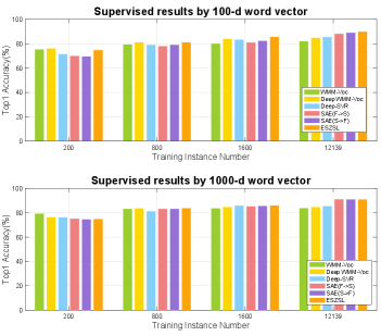
Supervised learning: The results are compared in Figure 4. As shown in the figure, we observe that our method shows significant improvements over the competitors in few-shot setting; however, as the number of instance increasing, the visual semantic mapping, , can be well learned, and the effects of additional vocabulary-informed constraints, become less pronounced.
Zero-shot learning: The ZSL results are compared in Figure 3. On all the settings, our two Voc methods – Deep WMM-Voc and WMM-Voc outperforms all the other baselines. This validates the importance of information learning from the open vocabulary. Further, we compare our results with the state-of-the-art ZSL results on AwA dataset in Table I. Our two models achieve and accuracy, which is markedly higher than all previous methods. This is particularly impressive, if we take into account the fact that we use only a semantic space and no additional attribute representations (unlike many other competitor methods). We argue that much of our success and improvement comes from a more discriminative information obtained using the open set vocabulary and corresponding large margin constraints, rather than from the features. Varying the number of training instances may slightly affect accuracy of methods reported in Table I. Therefore we report the best results of each competitor and our own method at different number of training instances .All competing methods in Figure 3 use the same features.
General zero-shot learning:. The general zero-shot learning results are compared in Table III. We consider the accuracies of both (Zero-shot-like) and (Supervised-like). In term of the harmonic mean , our methods have significantly better performance in the general zero-shot setting. This again shows that our framework can have better generalization by learning from the open vocabulary. On the other hand, in the terms of Area Under Seen-Unseen accuracy Curve (), the performance of Deep-SVR is very weak and the scores of ESZSL and SAE are lower than our method. Overall, the results of still support the superiority of our methods on G-ZSL tasks. Notably, since the source domain only have 24295 instances (including training and testing images), we are unable to obtain the results of Supervised-like setting (), and with all source instances.
| Metrics | ESZSL | SAE | Deep-SVR | WMM-Voc | Deep WMM-Voc | |
|---|---|---|---|---|---|---|
| 200 | 2.88/0 | 2.15/0 | 5.65/0 | 28.92/27.98 | 33.04/34.77 | |
| 75.76/76.08 | 70.13/75.32 | 71.22/76.32 | 70.20/74.20 | 71.16/69.48 | ||
| 5.55/0 | 4.17/0 | 10.47/0 | 40.96/40.64 | 45.13/46.35 | ||
| 0.4231/0.4344 | 0.3885/0.4556 | 0.3048/0.3939 | 0.4840/0.5190 | 0.5028/0.4776 | ||
| 800 | 0.19/0 | 0.78/0 | 5.34/0.02 | 25.57/25.68 | 27.59/27.77 | |
| 81.14/83.95 | 78.02/83.41 | 78.92/81.46 | 74.23/77.33 | 75.53/77.19 | ||
| 0.38/0 | 1.54/0 | 10.00/0.04 | 38.04/38.56 | 40.42/40.85 | ||
| 0.4409/0.4710 | 0.3870/0.4483 | 0.3452/0.4400 | 0.4764/0.5387 | 0.4953/0.5353 | ||
| 1600 | 0.71/0 | 0.87/0 | 4.69/0 | 24.63/27.22 | 33.66/32.86 | |
| 85.62/86.24 | 81.08/85.48 | 83.30/86.02 | 74.99/77.67 | 78.96/78.64 | ||
| 1.41/0 | 1.72/0 | 8.88/0 | 37.08/40.31 | 47.20/46.35 | ||
| 0.4507/0.5139 | 0.4190/0.4740 | 0.3776/0.4780 | 0.5016/0.5572 | 0.5554/0.5733 | ||
| 12139 | 0.37/0 | 0.44/0 | 5.19/0 | 27.80/30.53 | 32.23/28.19 | |
| 89.98/91.16 | 88.18/91.26 | 85.37/85.64 | 77.36/78.34 | 80.64/78.32 | ||
| 0.74/0 | 0.88/0 | 9.79/0 | 40.90/43.94 | 46.05/41.46 | ||
| 0.5096/0.5294 | 0.4493/0.5120 | 0.3353/0.4397 | 0.5144/0.5319 | 0.5525/0.5394 | ||
| 24295 | 0.83/0 | 0.37/0 | 5.39/0 | 27.15/29.42 | 35.65/31.78 | |
| - | - | - | - | - | ||
| - | - | - | - | - | ||
| - | - | - | - | - |
4.2.3 Large-scale open set recognition
We also compare the results on Open-set310K setting with the large vocabulary of approximately 310K entities; as such the chance performance is much lower. We use 100-dim word vector representations as the semantic space. While our Open-set variants do not assume that test data comes from either source/auxiliary domain or target domain, we split the two cases to mimic Supervised and Zero-shot scenarios for easier analysis. The results are shown in Figure 5.
On Supervised-like setting, Figure 5 (left), our Deep WMM-Voc and WMM-Voc have better performance than the other baselines. The better results are largely due to the better embedding matrix learned by enforcing maximum margins between training class name and open set vocabulary on source training data. This validates the effectiveness of proposed framework. In particular, we find that (1) The “deep” version always has better performance than their corresponding “non-deep” counterparts. For example, the Deep-SVR and Deep WMM-Voc achieve higher open-set recognition accuracy than SVR-Map and WMM-Voc. (2) The WMM-Voc has better performance than MM-Voc; this shows that the weighting strategy introduced in Section 3.4 can indeed help better learn the embedding from visual to semantic space.
On Zero shot-like setting, our method still has a notable advantage over that of SVR-Map, Deep-SVR methods on Top- () accuracy, again thanks to the better embedding learned by Eq. (10). However, we notice that our top-1 accuracy on Zero shot-like setting is lower than Deep SVR method. We find that our method tends to label some instances from target data with their nearest classes from within source label set. For example, “humpback whale” from testing data is more likely to be labeled as “blue whale”. However, when considering Top- () accuracy, our method still has advantages over baselines. It suggests that the semantic embeddings may be suffering from the problem that density of source classes is more concentrated than that of target classes. To show the effectiveness of WMM-Voc, as opposed to MM-Voc, we employ the False Positive Rate as the metric, , where means the number of testing unseen instances predicted as seen ones and defines the number of testing unseeen instances. Experiments are conducted on AwA dataset with all training instances, and 100-dim word vector prototypes. The false positive rates are , , , and by using SVR, Deep-SVR, MM-Voc, WMM-Voc and Deep WMM-Voc, respectively. They further validates that WMM-Voc outperforms MM-Voc.
|
|||||||||||||||
 |
|||||||||||||||
| Settings | SVR-Map | Deep-SVR | ESZSL | SAE | MM-Voc | WMM-Voc | Deep WMM-Voc |
|---|---|---|---|---|---|---|---|
| Supervised | 25.6/– | 31.26/50.51 | 38.26/64.38 | 32.95/54.44 | 37.1/62.35 | 35.95/62.77 | 38.92/65.35 |
| Zero-shot | 4.1/– | 5.29/13.32 | 5.86/13.71 | 5.11/12.62 | 8.90/14.90 | 8.50/20.73 | 9.26/21.99 |
4.3 Experimental results on ImageNet dataset
We validate our methods on large-scale ImageNet 2012/2010 dataset; the 1000-dimensional word2vec representation is used here since this dataset has larger number of classes than AwA. The instances of testing classes are equally sampled; making experiment less sensitive to the problem of unbalanced data. To be specific, testing instances from source classes are used in supervised, G-ZSL and open-set setting as well as testing instances from target classes are used in zero-shot, G-ZSL and open-set setting. The VGG-19 features of ImageNet pre-trained network are utilized as the input of all algorithms to make a fair comparison. We employ the Deep-SVR, SAE, ESZSL as baselines under the Supervised, Zero-shot and General Zero-shot settings respectively.
4.3.1 Pseudo-few-shot Source Training instances
The standard few-shot learning assumes disjoint instance set on source and target domains, as discussed in Sec. 4.3.2. As an ablation study, we would like to simulate a few-shot-like learning task on source domain by slightly violating the standard few-shot learning assumption. We name this setting “Pseudo-few-shot learning”: only few source training instances are used here and the feature extractor – VGG-19 model is pre-trained on ILSVRC 2012 dataset [12]. The “Pseudo-” here indicates that large amount of instances are used to train the feature extractor, but not used in training classifiers. Thus the experiments in this section can be served as an additional ablation study to reveal the insights of our model in addressing the few-shot-like task on source domain. Particularly, we conduct the experiments of using few-shot source training instance, i.e., 3,000 training instances used here. The results are listed in Table IV. We introduce this setting to particularly focus on learning from few training samples per class, in order to mimic human capability and performance in learning from few examples. We show that our vocabulary-informed learning framework enables learning with little data. In particular, we highlight that the Top-5 performance of WMM-Voc is much higher (>5%) than that of MM-Voc, despite the slightly worse performance on Top-1 accuracy. Note that the degradation of Top-1 results on ImageNet is also understandable. Note, WMM-Voc is only fitting the 3000 training instances on ImageNet dataset, and the features of these training instances may not be fine-tuned/optimized for the newly introduced penalty term of WMM-Voc. Once the features of training instances are fine-tuned by the deep version; we can show that the Deep WMM-Voc can improve from MM-Voc and WMM-Voc.
Critically, with different settings in Table IV, our vocabulary-informed learning can beat the other baselines under all settings. We highlight several findings:
(1) The supervised performance of our methods stands out from the state-of-art. Specifically, our Deep WMM-Voc achieves the highest supervised recognition accuracy, with ESZSL following closely. SVR-Map appears to be the worst.
(2) On Zero-shot learning task, our proposed Deep WMM-Voc gets 9.26% Top-1 and 21.99% Top-5 accuracy. It outperforms all the other baselines. Comparing with our previous MM-Voc result in [29], our result is 0.36% higher than MM-Voc. This improvement is statistically significant due to the few number of training instances and large number of testing instances. Additionally, the Top-1 result of WMM-Voc is 8.5% which is also comparable to that of MM-Voc, and far higher than those of SVR, Deep-SVR, ESZSL and SAE. This validates the effectiveness of learning from open vocabulary proposed in our two variants.
(3) In G-ZSL setting, we observe that both Deep WMM-Voc and WMM-Voc outperform all the other baselines. The full set of experiments on G-ZSL under different settings are reported in Table V.

| No. | Metrics | ESZSL | SAE | D-SVR | W-V | D-W-V |
|---|---|---|---|---|---|---|
| 0.46 | 0.24 | 0.20 | 2.02 | 1.93 | ||
| 38.07 | 32.86 | 31.06 | 32.40 | 36.61 | ||
| 0.91 | 0.48 | 0.40 | 3.80 | 3.67 | ||
| 0.38 | 0.18 | 0.18 | 2.01 | 1.99 | ||
| 49.65 | 46.23 | 33.54 | 32.87 | 43.53 | ||
| 0.75 | 0.36 | 0.36 | 3.79 | 3.81 | ||
| 0.37 | 0.19 | 0.20 | 2.11 | 2.15 | ||
| 57.43 | 54.55 | 36.75 | 33.16 | 47.28 | ||
| 0.74 | 0.38 | 0.40 | 3.97 | 4.11 |
4.3.2 Few-shot Target Training instances
We further introduce few-shot learning experiments on target instances to validate the performance of our methods. The experiments are conducted on ImageNet dataset. In total, there are 360 target classes from ImageNet 2010 data split with 100 instances per class; the feature extractor – VGG-19 is trained on the 1000 classes from ImageNet 2012. The 1 or 3 training instances are sampled from each target class. The other instances of the target classes are utilized as the test set. This is the few-shot learning setting, which is consistent with general definition [20]. We compare to SVM, KNN, Deep SVR, and SAE. The results are shown in Table VI. We can see that our method (WMM-Voc) can beat all the other competitors. Particularly, we have an obvious advantage in 1-shot target setting. Our Deep variant (Deep WMM-Voc) has better performance both in 1- and 3-shot setting. This shows the efficacy of proposed methods in few-shot learning task.
| Method | 1-instance | 3-instance |
|---|---|---|
| SVM | 2.65 | 9.81 |
| KNN | 5.23 | 13.3 |
| Deep SVR | 14.01 | 25.00 |
| SAE | 14.93 | 26.42 |
| WMM-Voc | 17.26 | 26.59 |
| Deep WMM-Voc | 17.95 | 30.44 |
4.3.3 Results on different training/testing splits
We further validate our findings on ImageNet 2012/2010 dataset. In general, our framework has advantages over the baselines since open vocabulary helps inform the learning process when few training instances or limited training data is available. The results are compared in Figure 6.
Supervised learning: As shown in Figure 6, we compare the supervised results by increasing the training instances from 3,000 to 50,000. With 3,000 training instances, the results of Deep WMM-Voc are better than all the other baselines with the help of learning from free vocabulary. We further evaluate our models with larger number of training instances (> 3 per class). We observe that for standard supervised learning setting, the improvements achieved using vocabulary-informed learning tend to somewhat diminish as the number of training instances substantially grows. With large number of training instances, the mapping between low-level image features and semantic words, , becomes better behaved and effect of additional constraints, due to the open-vocabulary, becomes less pronounced.
Zero-shot Learning: We further validate the results on zero-shot learning setting. Figure 6 shows that our models can beat all other baselines. Our Deep WMM-Voc always performs the best with the source training instances increased from 3,000 to 50,000. The WMM-Voc always has the second best performance; especially when only few source training instances are available, i.e., 3,000 and 5,000 training instances. Our Deep WMM-Voc and WMM-Voc demonstrate significant improvements over the competitors in ZSL task. The good performance of Deep WMM-Voc and WMM-Voc is largely due to our vocabulary-informed learning framework which can leverage the discriminative information from open vocabulary and max-margin constraints, helping to improve performance.
General Zero-shot Learning: In G-ZSL, our methods still have the best performance compared to the baselines, as seen from Table V. The Top-1 results of WMM-Voc and Deep WMM-Voc are beyond 2%; in contrast, the performance of other state-of-art methods are lower than 0.5%.
| Methods | S. Sp | T-1 | T-5 |
| Deep WMM-Voc | W | 9.26/10.29 | 21.99/23.12 |
| WMM-Voc | W | 8.5/8.76 | 20.30/21.36 |
| MM-Voc | W | 8.9/9.5 | 14.9/16.8 |
| SAE | W | 5.11/9.32 | 12.26/21.04 |
| ESZSL | W | 5.86/8.3 | 13.71/18.2 |
| Deep-SVR | W | 5.29/5.7 | 13.32/14.12 |
| Embed [88] | W | –/11.00 | –/25.70 |
| ConSE [53] | W | 5.5/7.8 | 13.1/15.5 |
| DeViSE [24] | W | 3.7/5.2 | 11.8/12.8 |
| AMP [31] | W | 3.5/6.1 | 10.5/13.1 |
| Chance | – | – |
Varying training set size: In Figure 6 we also evaluate our model with the larger number of training instances ( per class) in all settings. The results are inline with prior findings.
The state-of-the-art on ZSL: We compare our results to several state-of-the-art large-scale zero-shot recognition models. Our results are better than those of ConSE, DeViSE, Deep-SVR, SAE, ESZSL and AMP on both T-1 and T-5 metrics with a very significant margin. Poor results of DeViSE with training instances are largely due to the inefficient learning of visual-semantic embedding matrix. AMP algorithm also relies on the embedding matrix from DeViSE, which explains similar poor performance of AMP with training instances. Table VII shows that our Deep WMM-Voc obtains good performance with (all) 50,000 training instances. Top-5 accuracy of our methods are beyond 20%. This again validates that our proposed methods can have the advantages of learning from limited available training instances by leveraging the discriminative information from open vocabulary. Embed [1] has slightly better ZSL performance compared to our models. However, unlike the other works that directly use word vector representations of class names, [1] require additional textual descriptions of each class to learn better class prototypes.
Open-set recognition: The open set image recognition results are shown in Figure 7. On Supervised-like settings, we notice the MM-Voc and WMM-Voc have similar open set recognition accuracy. Since this dataset is very large, linear mapping may not have enough capacity to model the embedding mapping from visual space to semantic space. Thus adding constraints on source training classes in WMM-Voc may slightly hinder the learning such an embedding. That explains why the results of WMM-Voc are slightly inferior to MM-Voc. Deep WMM-Voc has the best performance, due to its ability to fine-tune low-level feature representation while learning the embedding. On the Zero-shot-like setting, our WMM-Voc and Deep WMM-Voc have the best performance.
| Testing Classes | ||||
| ImageNet Data | Aux. | Tag. | Total | Vocab |
| Open-Set310K | (left) | (right) | 1000 / 360 | |

Qualitative visualization: We illustrate the embedding space learned by our Deep WMM-Voc model for the ImageNet2012/2010 dataset in Figure 1. In particular, we have 4 source/auxiliary and 2 target/zero-shot classes in this figure. The better separation among classes is largely attributed to open-set max-margin constraints introduced in our vocabulary-informed learning model. We further visualize the semantic space in Figure 8. Critically, we list seven target classes on AwA dataset, as well as their surrounding neighborhood open vocabulary. For example, “orcas” is very near to “killer_whale”. While “orcas” are semantically different from “killer_whale”, the difference is much smaller if we compare the “orcas” with the other classes, such as “spider monkey”, “grizzly_bear” and so on. Hence the “orcas” can be used to help learn the class of “killer_whale” in our vocabulary-informed learning framework.

5 Conclusion and Future Work
This paper introduces the learning paradigm of vocabulary-informed learning, by utilizing open set semantic vocabulary to help train better classifiers for observed and unobserved classes in supervised learning, ZSL, G-ZSL, and open set image recognition settings. We formulate vocabulary-informed learning in the maximum margin frameworks. Extensive experimental results illustrate the efficacy of such learning paradigm. Strikingly, it achieves competitive performance with very few training instances and is relatively robust to a large open set vocabulary of up to class labels.
Acknowledgments
This work was supported in part by NSFC Project (61702108, 61622204), STCSM Project (16JC1420400), Eastern Scholar (TP2017006), Shanghai Municipal Science and Technology Major Project (2017SHZDZX01, 2018SHZDZX01) and ZJLab.
References
- [1]
- [2] Z. Akata, F. Perronnin, Z. Harchaoui, and C. Schmid. Label-embedding for image classification. IEEE transactions on pattern analysis and machine intelligence, 38(7):1425–1438, 2015.
- [3] Z. Akata, S. Reed, D. Walter, H. Lee, and B. Schiele. Evaluation of output embeddings for fine-grained image classification. In Proceedings of the IEEE Conference on Computer Vision and Pattern Recognition, pages 2927–2936, 2015.
- [4] Y. Amit, M. Fink, N. Srebro, and S. Ullman. Uncovering shared structures in multiclass classification. In Proceedings of the 24th international conference on Machine learning, pages 17–24. ACM, 2007.
- [5] E. Bart and S. Ullman. Cross-generalization: Learning novel classes from a single example by feature replacement. In 2005 IEEE Computer Society Conference on Computer Vision and Pattern Recognition (CVPR’05), volume 1, pages 672–679. IEEE, 2005.
- [6] A. Bendale and T. Boult. Towards open world recognition. In Proceedings of the IEEE Conference on Computer Vision and Pattern Recognition, pages 1893–1902, 2015.
- [7] A. Bendale and T. Boult. Towards open set deep networks. In Computer Vision and Pattern Recognition, 2016 IEEE Conference on. IEEE, 2016.
- [8] I. Biederman. Recognition-by-components: a theory of human image understanding. Psychological review, 94(2):115, 1987.
- [9] S. Changpinyo, W.-L. Chao, B. Gong, and F. Sha. Synthesized classifiers for zero-shot learning. In Proceedings of the IEEE Conference on Computer Vision and Pattern Recognition, pages 5327–5336, 2016.
- [10] S. Changpinyo, W.-L. Chao, and F. Sha. Predicting visual exemplars of unseen classes for zero-shot learning. In Proceedings of the IEEE International Conference on Computer Vision, pages 3476–3485, 2017.
- [11] W.-L. Chao, S. Changpinyo, B. Gong, and F. Sha. An empirical study and analysis of generalized zero-shot learning for object recognition in the wild. In European Conference on Computer Vision, pages 52–68. Springer, 2016.
- [12] K. Chatfield, K. Simonyan, A. Vedaldi, and A. Zisserman. Return of the devil in the details: Delving deep into convolutional nets. arXiv preprint arXiv:1405.3531, 2014.
- [13] K. Crammer and Y. Singer. On the algorithmic implementation of multiclass kernel-based vector machines. Journal of machine learning research, 2(Dec):265–292, 2001.
- [14] J. Deng, N. Ding, Y. Jia, A. Frome, K. Murphy, S. Bengio, Y. Li, H. Neven, and H. Adam. Large-scale object classification using label relation graphs. In European conference on computer vision, pages 48–64. Springer, 2014.
- [15] J. Deng, W. Dong, R. Socher, L.-J. Li, K. Li, and L. Fei-Fei. Imagenet: A large-scale hierarchical image database. In 2009 IEEE conference on computer vision and pattern recognition, pages 248–255. IEEE, 2009.
- [16] G. Dinu, A. Lazaridou, and M. Baroni. Improving zero-shot learning by mitigating the hubness problem. arXiv preprint arXiv:1412.6568, 2014.
- [17] H. Dong, Y. Fu, L. Sigal, S. J. Hwang, Y.-G. Jiang, and X. Xue. Learning to separate domains in generalized zero-shot and open set learning: a probabilistic perspective. arXiv preprint arXiv:1810.07368, 2018.
- [18] A. Farhadi, I. Endres, D. Hoiem, and D. Forsyth. Describing objects by their attributes. In 2009 IEEE Conference on Computer Vision and Pattern Recognition, pages 1778–1785. IEEE, 2009.
- [19] L. Fei-Fei, R. Fergus, and P. Perona. A bayesian approach to unsupervised one-shot learning of object categories. In IEEE International Conference on Computer Vision, 2003.
- [20] L. Fei-Fei, R. Fergus, and P. Perona. One-shot learning of object categories. IEEE Trans. Pattern Anal. Mach. Intell., 28(4):594–611, Apr. 2006.
- [21] R. Felix, B. Vijay Kumar, I. Reid, and G. Carneiro. Multi-modal cycle-consistent generalized zero-shot learning. In Proceedings of the European Conference on Computer Vision, pages 21–37, 2018.
- [22] F. Fleuret and G. Blanchard. Pattern recognition from one example by chopping. In Advances in Neural Information Processing Systems, pages 371–378, 2006.
- [23] M. P. Friedlander and M. Schmidt. Hybrid deterministic-stochastic methods for data fitting. SIAM Journal on Scientific Computing, 34(3):A1380–A1405, 2012.
- [24] A. Frome, G. S. Corrado, J. Shlens, S. Bengio, J. Dean, T. Mikolov, et al. Devise: A deep visual-semantic embedding model. In Advances in neural information processing systems, pages 2121–2129, 2013.
- [25] Y. Fu, T. M. Hospedales, T. Xiang, Z. Fu, and S. Gong. Transductive multi-view embedding for zero-shot recognition and annotation. In European Conference on Computer Vision, pages 584–599. Springer, 2014.
- [26] Y. Fu, T. M. Hospedales, T. Xiang, and S. Gong. Attribute learning for understanding unstructured social activity. In European Conference on Computer Vision, pages 530–543. Springer, 2012.
- [27] Y. Fu, T. M. Hospedales, T. Xiang, and S. Gong. Learning multimodal latent attributes. IEEE transactions on pattern analysis and machine intelligence, 36(2):303–316, 2013.
- [28] Y. Fu, T. M. Hospedales, T. Xiang, and S. Gong. Transductive multi-view zero-shot learning. IEEE transactions on pattern analysis and machine intelligence, 37(11):2332–2345, 2015.
- [29] Y. Fu and L. Sigal. Semi-supervised vocabulary-informed learning. In Proceedings of the IEEE Conference on Computer Vision and Pattern Recognition, pages 5337–5346, 2016.
- [30] Y. Fu, T. Xiang, Y.-G. Jiang, X. Xue, L. Sigal, and S. Gong. Recent advances in zero-shot recognition: Toward data-efficient understanding of visual content. IEEE Signal Processing Magazine, 35(1):112–125, 2018.
- [31] Z. Fu, T. Xiang, E. Kodirov, and S. Gong. Zero-shot object recognition by semantic manifold distance. In Proceedings of the IEEE conference on computer vision and pattern recognition, pages 2635–2644, 2015.
- [32] S. Guadarrama, E. Rodner, K. Saenko, N. Zhang, R. Farrell, J. Donahue, and T. Darrell. Open-vocabulary object retrieval. In Robotics: science and systems, volume 2, page 6, 2014.
- [33] T. Hertz, A. B. Hillel, and D. Weinshall. Learning a kernel function for classification with small training samples. In Proceedings of the 23rd international conference on Machine learning, pages 401–408. ACM, 2006.
- [34] A. G. Huth, S. Nishimoto, A. T. Vu, and J. L. Gallant. A continuous semantic space describes the representation of thousands of object and action categories across the human brain. Neuron, 76(6):1210–1224, 2012.
- [35] S. J. Hwang and L. Sigal. A unified semantic embedding: Relating taxonomies and attributes. In Advances in Neural Information Processing Systems, pages 271–279, 2014.
- [36] D. Jayaraman and K. Grauman. Zero-shot recognition with unreliable attributes. In Advances in neural information processing systems, pages 3464–3472, 2014.
- [37] G. Koch, R. Zemel, and R. Salakhutdinov. Siamese neural networks for one-shot image recognition. In ICML deep learning workshop, volume 2, 2015.
- [38] E. Kodirov, T. Xiang, and S. Gong. Semantic autoencoder for zero-shot learning. In Proceedings of the IEEE Conference on Computer Vision and Pattern Recognition, pages 3174–3183, 2017.
- [39] S. Kotz, N. Balakrishnan, and N. L. Johnson. Continuous multivariate distributions, Volume 1: Models and applications, volume 1. John Wiley & Sons, 2004.
- [40] S. Kotz and S. Nadarajah. Extreme value distributions: theory and applications. World Scientific, 2000.
- [41] A. Krizhevsky, I. Sutskever, and G. E. Hinton. Imagenet classification with deep convolutional neural networks. In Advances in neural information processing systems, pages 1097–1105, 2012.
- [42] N. Kumar, A. C. Berg, P. N. Belhumeur, and S. K. Nayar. Attribute and simile classifiers for face verification. In 2009 IEEE 12th International Conference on Computer Vision, pages 365–372. IEEE, 2009.
- [43] C. H. Lampert, H. Nickisch, and S. Harmeling. Attribute-based classification for zero-shot visual object categorization. IEEE Transactions on Pattern Analysis and Machine Intelligence, 36(3):453–465, 2014.
- [44] H. Larochelle, D. Erhan, and Y. Bengio. Zero-data learning of new tasks. In AAAI, volume 1, page 3, 2008.
- [45] A. Lazaridou, G. Dinu, and M. Baroni. Hubness and pollution: Delving into cross-space mapping for zero-shot learning. In Proceedings of the 53rd Annual Meeting of the Association for Computational Linguistics and the 7th International Joint Conference on Natural Language Processing (Volume 1: Long Papers), volume 1, pages 270–280, 2015.
- [46] Y.-J. Lee, W.-F. Hsieh, and C.-M. Huang. epsilon-ssvr: A smooth support vector machine for epsilon-insensitive regression. IEEE Transactions on Knowledge & Data Engineering, (5):678–685, 2005.
- [47] T. Long, X. Xu, Y. Li, F. Shen, J. Song, and H. T. Shen. Pseudo transfer with marginalized corrupted attribute for zero-shot learning. In 2018 ACM Multimedia Conference on Multimedia Conference, pages 4281–4289. ACM, 2018.
- [48] T. Long, X. Xu, F. Shen, L. Liu, N. Xie, and Y. Yang. Zero-shot learning via discriminative representation extraction. Pattern Recognition Letters, 109:27–34, 2018.
- [49] Y. Long, L. Liu, L. Shao, F. Shen, G. Ding, and J. Han. From zero-shot learning to conventional supervised classification: Unseen visual data synthesis. In Proceedings of the IEEE Conference on Computer Vision and Pattern Recognition, pages 1627–1636, 2017.
- [50] Y. Long, L. Liu, F. Shen, L. Shao, and X. Li. Zero-shot learning using synthesised unseen visual data with diffusion regularisation. IEEE Transactions on Pattern Analysis and Machine Intelligence, 40(10):2498–2512, 2018.
- [51] C. Manning, P. Raghavan, and H. Schütze. Introduction to information retrieval. Natural Language Engineering, 16(1):100–103, 2010.
- [52] T. Mikolov, I. Sutskever, K. Chen, G. S. Corrado, and J. Dean. Distributed representations of words and phrases and their compositionality. In Advances in neural information processing systems, pages 3111–3119, 2013.
- [53] M. Norouzi, T. Mikolov, S. Bengio, Y. Singer, J. Shlens, A. Frome, G. S. Corrado, and J. Dean. Zero-shot learning by convex combination of semantic embeddings. arXiv preprint arXiv:1312.5650, 2013.
- [54] M. Palatucci, D. Pomerleau, G. E. Hinton, and T. M. Mitchell. Zero-shot learning with semantic output codes. In Advances in neural information processing systems, pages 1410–1418, 2009.
- [55] S. J. Pan and Q. Yang. A survey on transfer learning. IEEE Transactions on Data and Knowledge Engineering, 22(10):1345–1359, 2010.
- [56] D. Parikh and K. Grauman. Relative attributes. In 2011 International Conference on Computer Vision, pages 503–510. IEEE, 2011.
- [57] J. Pennington, R. Socher, and C. Manning. Glove: Global vectors for word representation. In Proceedings of the 2014 conference on empirical methods in natural language processing (EMNLP), pages 1532–1543, 2014.
- [58] M. Rohrbach, S. Ebert, and B. Schiele. Transfer learning in a transductive setting. In Advances in neural information processing systems, pages 46–54, 2013.
- [59] M. Rohrbach, M. Stark, and B. Schiele. Evaluating knowledge transfer and zero-shot learning in a large-scale setting. In CVPR 2011, pages 1641–1648. IEEE, 2011.
- [60] M. Rohrbach, M. Stark, G. Szarvas, I. Gurevych, and B. Schiele. What helps where–and why? semantic relatedness for knowledge transfer. In 2010 IEEE Computer Society Conference on Computer Vision and Pattern Recognition, pages 910–917. IEEE, 2010.
- [61] B. Romera-Paredes and P. Torr. An embarrassingly simple approach to zero-shot learning. In International Conference on Machine Learning, pages 2152–2161, 2015.
- [62] E. M. Rudd, L. P. Jain, W. J. Scheirer, and T. E. Boult. The extreme value machine. IEEE transactions on pattern analysis and machine intelligence, 40(3):762–768, 2017.
- [63] H. Sattar, S. Muller, M. Fritz, and A. Bulling. Prediction of search targets from fixations in open-world settings. In Proceedings of the IEEE Conference on Computer Vision and Pattern Recognition, pages 981–990, 2015.
- [64] R. E. Schapire, Y. Freund, P. Bartlett, W. S. Lee, et al. Boosting the margin: A new explanation for the effectiveness of voting methods. The annals of statistics, 26(5):1651–1686, 1998.
- [65] W. J. Scheirer, L. P. Jain, and T. E. Boult. Probability models for open set recognition. IEEE transactions on pattern analysis and machine intelligence, 36(11):2317–2324, 2014.
- [66] W. J. Scheirer, A. Rocha, A. Sapkota, and T. E. Boult. Towards open set recognition. IEEE Transactions on Pattern Analysis and Machine Intelligence, 2013.
- [67] Y. Shigeto, I. Suzuki, K. Hara, M. Shimbo, and Y. Matsumoto. Ridge regression, hubness, and zero-shot learning. In Joint European Conference on Machine Learning and Knowledge Discovery in Databases, pages 135–151. Springer, 2015.
- [68] R. Socher, M. Ganjoo, C. D. Manning, and A. Ng. Zero-shot learning through cross-modal transfer. In Advances in neural information processing systems, pages 935–943, 2013.
- [69] F. Sung, Y. Yang, L. Zhang, T. Xiang, P. H. Torr, and T. M. Hospedales. Learning to compare: Relation network for few-shot learning. In Proceedings of the IEEE Conference on Computer Vision and Pattern Recognition, pages 1199–1208, 2018.
- [70] S. Thrun. Learning to learn: Introduction. 1996.
- [71] T. Tommasi and B. Caputo. The more you know, the less you learn: from knowledge transfer to one-shot learning of object categories. Technical report, 2009.
- [72] A. Torralba, R. Fergus, and W. T. Freeman. 80 million tiny images: A large data set for nonparametric object and scene recognition. IEEE transactions on pattern analysis and machine intelligence, 30(11):1958–1970, 2008.
- [73] A. Torralba, K. P. Murphy, and W. T. Freeman. Sharing visual features for multiclass and multiview object detection. IEEE Transactions on Pattern Analysis & Machine Intelligence, (5):854–869, 2007.
- [74] A. Torralba, K. P. Murphy, and W. T. Freeman. Using the forest to see the trees: exploiting context for visual object detection and localization. Communications of the ACM, 53(3):107–114, 2010.
- [75] I. Tsochantaridis, T. Joachims, T. Hofmann, and Y. Altun. Large margin methods for structured and interdependent output variables. Journal of machine learning research, 6(Sep):1453–1484, 2005.
- [76] A. Vedaldi and A. Zisserman. Efficient additive kernels via explicit feature maps. In IEEE Transactions on Pattern Analysis and Machine Intelligence, 2011.
- [77] V. K. Verma, G. Arora, A. Mishra, and P. Rai. Generalized zero-shot learning via synthesized examples. In Proc. 31th IEEE Conf. Comput. Vis. Pattern Recognit., pages 4281–4289, 2018.
- [78] V. K. Verma and P. Rai. A simple exponential family framework for zero-shot learning. In Joint European Conference on Machine Learning and Knowledge Discovery in Databases, pages 792–808. Springer, 2017.
- [79] R. Vilalta and Y. Drissi. A perspective view and survey of meta-learning. Artificial intelligence review, 18(2):77–95, 2002.
- [80] J. Weston, S. Bengio, and N. Usunier. Wsabie: Scaling up to large vocabulary image annotation. In Twenty-Second International Joint Conference on Artificial Intelligence, 2011.
- [81] L. Wolf and I. Martin. Robust boosting for learning from few examples. In 2005 IEEE Computer Society Conference on Computer Vision and Pattern Recognition (CVPR’05), volume 1, pages 359–364. IEEE, 2005.
- [82] Z. Wu, Y. Fu, Y.-G. Jiang, and L. Sigal. Harnessing object and scene semantics for large-scale video understanding. In Proceedings of the IEEE Conference on Computer Vision and Pattern Recognition, pages 3112–3121, 2016.
- [83] Y. Xian, Z. Akata, G. Sharma, Q. Nguyen, M. Hein, and B. Schiele. Latent embeddings for zero-shot classification. In Proceedings of the IEEE Conference on Computer Vision and Pattern Recognition, pages 69–77, 2016.
- [84] Y. Xian, T. Lorenz, B. Schiele, and Z. Akata. Feature generating networks for zero-shot learning. In Proceedings of the IEEE conference on computer vision and pattern recognition, pages 5542–5551, 2018.
- [85] Y. Xian, B. Schiele, and Z. Akata. Zero-shot learning-the good, the bad and the ugly. In Proceedings of the IEEE Conference on Computer Vision and Pattern Recognition, pages 4582–4591, 2017.
- [86] F. X. Yu, L. Cao, R. S. Feris, J. R. Smith, and S.-F. Chang. Designing category-level attributes for discriminative visual recognition. In Proceedings of the IEEE Conference on Computer Vision and Pattern Recognition, pages 771–778, 2013.
- [87] Y. Yu, Z. Ji, J. Guo, and Y. Pang. Transductive zero-shot learning with adaptive structural embedding. IEEE Transactions on Neural Networks and Learning Systems, 29(9):4116–4127, 2018.
- [88] L. Zhang, T. Xiang, and S. Gong. Learning a deep embedding model for zero-shot learning. In Proceedings of the IEEE Conference on Computer Vision and Pattern Recognition, pages 2021–2030, 2017.
- [89] T. Zhang. Solving large scale linear prediction problems using stochastic gradient descent algorithms. In Proceedings of the twenty-first international conference on Machine learning, page 116. ACM, 2004.
- [90] T. Zhang and Z.-H. Zhou. Large margin distribution machine. In Proceedings of the 20th ACM SIGKDD international conference on Knowledge discovery and data mining, pages 313–322. ACM, 2014.
- [91] Z. Zhang and V. Saligrama. Zero-shot learning via semantic similarity embedding. In Proceedings of the IEEE international conference on computer vision, pages 4166–4174, 2015.
- [92] Z.-H. Zhou. Large margin distribution learning. In IAPR Workshop on Artificial Neural Networks in Pattern Recognition, pages 1–11. Springer, 2014.
![[Uncaptioned image]](https://cdn.awesomepapers.org/papers/c2d86c23-9f4a-4621-84ac-67ebeabc92a1/x9.png) |
Yanwei Fu received the Ph.D. degree from Queen Mary University of London in 2014, and the M.Eng. degree from the Department of Computer Science and Technology, Nanjing University, China, in 2011. He held a post-doctoral position at Disney Research, Pittsburgh, PA, USA, from 2015 to 2016. He is currently a tenure-track Professor with Fudan University. His research interests are image and video understanding, and life-long learning. |
![[Uncaptioned image]](https://cdn.awesomepapers.org/papers/c2d86c23-9f4a-4621-84ac-67ebeabc92a1/x10.png) |
Xiaomei Wang is a PhD student in the School of Computer Science of Fudan University. She received the Master degree of communication and information system from Shanghai University in 2016 and the Bachelor degree of electronic information engineering from Shandong University of Technology in 2012. Her reaseach interests include zero-shot/few-shot learning, image/video captioning and visual question answering. |
![[Uncaptioned image]](https://cdn.awesomepapers.org/papers/c2d86c23-9f4a-4621-84ac-67ebeabc92a1/x11.png) |
Hanze Dong is an undergraduate student majoring in mathematics (data science track) at the School of Data Science, Fudan University. He works in Shanghai Key Lab of Intelligent Information Processing under the supervision of Professor Yanwei Fu. His current research interests include both machine learning theory and its applications. |
![[Uncaptioned image]](https://cdn.awesomepapers.org/papers/c2d86c23-9f4a-4621-84ac-67ebeabc92a1/x12.png) |
Yu-Gang Jiang is Professor of Computer Science at Fudan University and Director of Fudan-Jilian Joint Research Center on Intelligent Video Technology, Shanghai, China. He is interested in all aspects of extracting high-level information from big video data, such as video event recognition, object/scene recognition and large-scale visual search. His work has led to many awards, including the inaugural ACM China Rising Star Award, the 2015 ACM SIGMM Rising Star Award, and the research award for outstanding young researchers from NSF China. He is currently an associate editor of ACM TOMM, Machine Vision and Applications (MVA) and Neurocomputing. He holds a PhD in Computer Science from City University of Hong Kong and spent three years working at Columbia University before joining Fudan in 2011. |
![[Uncaptioned image]](https://cdn.awesomepapers.org/papers/c2d86c23-9f4a-4621-84ac-67ebeabc92a1/x13.png) |
Meng Wang is a professor at the Hefei University of Technology, China. He received his B.E. degree and Ph.D. degree in the Special Class for the Gifted Young and the Department of Electronic Engineering and Information Science from the University of Science and Technology of China (USTC), Hefei, China, in 2003 and 2008, respectively. His current research interests include multimedia content analysis, computer vision, and pattern recognition. He has authored more than 200 book chapters, journal and conference papers in these areas. He is the recipient of the ACM SIGMM Rising Star Award 2014. He is an associate editor of IEEE Transactions on Knowledge and Data Engineering (IEEE TKDE), IEEE Transactions on Circuits and Systems for Video Technology (IEEE TCSVT), IEEE Transactions on Multimedia (IEEE TMM), and IEEE Transactions on Neural Networks and Learning Systems (IEEE TNNLS). |
![[Uncaptioned image]](https://cdn.awesomepapers.org/papers/c2d86c23-9f4a-4621-84ac-67ebeabc92a1/x14.png) |
Xiangyang Xue received the BS, MS, and PhD degrees in communication engineering from Xidian University, Xi’an, China, in 1989, 1992, and 1995, respectively. He is currently a professor of computer science with Fudan University, Shanghai, China. His research interests include computer vision, multimedia information processing and machine learning. |
![[Uncaptioned image]](https://cdn.awesomepapers.org/papers/c2d86c23-9f4a-4621-84ac-67ebeabc92a1/x15.png) |
Leonid Sigal is an Associate Professor in the Department of Computer Science at the University of British Columbia and a Faculty Member of the Vector Institute for Artificial Intelligence. He is a recipient of Canada CIFAR AI Chair and NSERC Canada Research Chair (CRC) in Computer Vision and Machine Learning. Prior to this he was a Senior Research Scientist at Disney Research. He completed his Ph.D. at Brown University in 2008; received his M.A. from Boston University in 1999, and M.Sc. from Brown University in 2003. Leonid’s research interests lie in the areas of computer vision, machine learning, and computer graphics. Leonid’s research emphasis is on machine learning and statistical approaches for visual recognition, reasoning, understanding and analytics. He has published more than 70 papers in venues and journals in these fields (including TPAMI, IJCV, CVPR, ICCV and NeurIPS). |