linecolor=gray,linewidth=1pt
Visualizing the Obvious: A Concreteness-based Ensemble Model
for Noun Property Prediction
Abstract
Neural language models encode rich knowledge about entities and their relationships which can be extracted from their representations using probing. Common properties of nouns (e.g., red strawberries, small ant) are, however, more challenging to extract compared to other types of knowledge because they are rarely explicitly stated in texts. We hypothesize this to mainly be the case for perceptual properties which are obvious to the participants in the communication. We propose to extract these properties from images and use them in an ensemble model, in order to complement the information that is extracted from language models. We consider perceptual properties to be more concrete than abstract properties (e.g., interesting, flawless). We propose to use the adjectives’ concreteness score as a lever to calibrate the contribution of each source (text vs. images). We evaluate our ensemble model in a ranking task where the actual properties of a noun need to be ranked higher than other non-relevant properties. Our results show that the proposed combination of text and images greatly improves noun property prediction compared to powerful text-based language models.111Code and data are available at https://github.com/artemisp/semantic-norms
1 Introduction
Common properties of concepts or entities (e.g., “These strawberries are red”) are rarely explicitly stated in texts, contrary to more specific properties which bring new information in the communication (e.g., “These strawberries are delicious”). This phenomenon, known as “reporting bias” Gordon and Van Durme (2013); Shwartz and Choi (2020), makes it difficult to learn, or retrieve, perceptual properties from text. However, noun property identification is an important task which may allow AI applications to perform commonsense reasoning in a way that matches people’s psychological or cognitive predispositions and can improve agent communication (Lazaridou et al., 2016). Furthermore, identifying noun properties can contribute to better modeling concepts and entities, learning affordances (i.e. defining the possible uses of an object based on its qualities or properties), and understanding models’ knowledge about the world. Models that combine different modalities provide a sort of grounding which helps to alleviate the reporting bias problem Kiela et al. (2014); Lazaridou et al. (2015); Zhang et al. (2022). For example, multimodal models are better at predicting color attributes compared to text-based language models Paik et al. (2021); Norlund et al. (2021). Furthermore, visual representations of concrete objects improve performance in downstream NLP tasks Hewitt et al. (2018). Inspired by this line of work, we expect concrete visual properties of nouns to be more accessible through images, and text-based language models to better encode abstract semantic properties. We propose an ensemble model which combines information from these two sources for English noun property prediction.
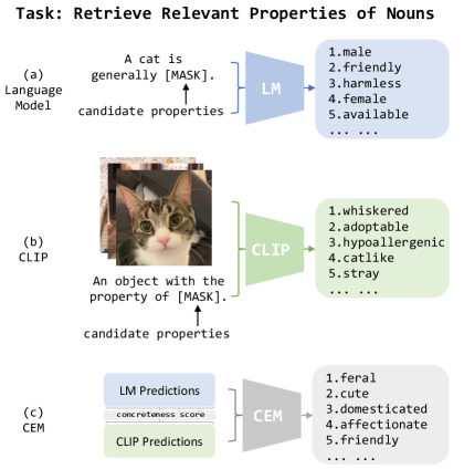
We frame property identification as a ranking task, where relevant properties for a noun need to be retrieved from a set of candidate properties found in association norm datasets McRae et al. (2005); Devereux et al. (2014); Norlund et al. (2021). We experiment with text-based language models Devlin et al. (2019); Radford et al. (2019); Liu et al. (2019) and with CLIP Radford et al. (2021) which we query using a slot filling task, as shown in Figures 1(a) and (b). Our ensemble model (Figure 1(c)) combines the strengths of the language and vision models, by specifically privileging the former or latter type of representation depending on the concreteness of the processed properties Brysbaert et al. (2014). Given that concrete properties are characterized by a higher degree of imageability Friendly et al. (1982), our model trusts the visual model for perceptual and highly concrete properties (e.g., color adjectives: red, green), and the language model for abstract properties (e.g., free, infinite). Our results confirm that CLIP can identify nouns’ perceptual properties better than language models, which contain higher-quality information about abstract properties. Our ensemble model, which combines the two sources of knowledge, outperforms the individual models on the property ranking task by a significant margin.
2 Related Work
Probing has been widely used in previous work for exploring the semantic knowledge that is encoded in language models. A common approach has been to convert the facts, properties, and relations found in external knowledge sources into “fill-in-the-blank” cloze statements, and to use them to query language models. Apidianaki and Garí Soler (2021) do so for nouns’ semantic properties and highlight how challenging it is to retrieve this kind of information from BERT representations Devlin et al. (2019).
Furthermore, slightly different prompts tend to retrieve different semantic information (Ettinger, 2020), compromising the robustness of semantic probing tasks. We propose to mitigate these problems by also relying on images.
Features extracted from different modalities can complement the information found in texts. Multimodal distributional models, for example, have been shown to outperform text-based approaches on semantic benchmarks Silberer et al. (2013); Bruni et al. (2014); Lazaridou et al. (2015). Similarly, ensemble models that integrate multimodal and text-based models outperform models that only rely on one modality in tasks such as visual question answering Tsimpoukelli et al. (2021); Alayrac et al. (2022); Yang et al. (2021b), visual entailment Song et al. (2022), reading comprehension, natural language inference Zhang et al. (2021); Kiros et al. (2018), text generation Su et al. (2022), word sense disambiguation Barnard and Johnson (2005), and video retrieval Yang et al. (2021a).
We extend this investigation to noun property prediction. We propose a novel noun property retrieval model which combines information from language and vision models, and tunes their respective contributions based on property concreteness Brysbaert et al. (2014).
Concreteness is a graded notion that strongly correlates with the degree of imageability Friendly et al. (1982); Byrne (1974); concrete words generally tend to refer to tangible objects that the senses can easily perceive Paivio et al. (1968). We extend this idea to noun properties and hypothesize that vision models would have better knowledge of perceptual, and more concrete, properties (e.g., red, flat, round) than text-based language models, which would better capture abstract properties (e.g., free, inspiring, promising). We evaluate our ensemble model using concreteness scores automatically predicted by a regression model Charbonnier and Wartena (2019). We compare these results to the performance of the ensemble model with manual (gold) concreteness ratings Brysbaert et al. (2014). In previous work, concreteness was measured based on the idea that abstract concepts relate to varied and composite situations (Barsalou and Wiemer-Hastings, 2005). Consequently, visually grounded representations of abstract concepts (e.g., freedom) should be more complex and diverse than those of concrete words (e.g., dog) Lazaridou et al. (2015); Kiela et al. (2014).
Lazaridou et al. (2015) specifically measure the entropy of the vectors induced by multimodal models which serve as an expression of how varied the information they encode is. They demonstrate that the entropy of multimodal vectors strongly correlates with the degree of abstractness of words.
3 Experimental Setup
3.1 Task Formulation
Given a noun and a set of candidate properties , a model needs to select the properties that apply to . The candidate properties are the set of all adjectives retained from a resource (cf. Section 3.2), which characterize different nouns. A model needs to rank properties that apply to higher than properties that apply to other nouns in the resource. We consider that a property correctly characterizes a noun, if this property has been proposed for that noun by the annotators.
3.2 Datasets
Feature Norms: The McRae et al. (2005) dataset contains feature norms for 541 objects annotated by 725 participants. We follow Apidianaki and Garí Soler (2021) and only use the is_adj features of noun concepts, where the adjective describes a noun property. In total, there are 509 noun concepts with at least one is_adj feature, and 209 unique properties. The Feature Norms dataset contains both perceptual properties (e.g., tall, fluffy) and non-perceptual ones (e.g., intelligent, expensive).
Memory Colors: The dataset contains 109 nouns with an associated image and its corresponding prototypical color. There are 11 colors in total. Norlund et al. (2021). The data were scraped from existing knowledge bases on the web.
Concept Properties: This dataset was created at the Centre for Speech, Language and Brain Devereux et al. (2014). It contains concept property norm annotations collected from 30 participants. The data comprise 601 nouns with 400 unique properties. We keep aside 50 nouns (which are not in Feature Norms and Memory Colors) as our development set (dev). We use the dev for prompt selection and hyper-parameter tuning. We call the rest of the dataset Concept Properties-test and use it for evaluation.
Concreteness Dataset: The Brysbaert et al. (2014) dataset contains manual concreteness ratings for 37,058 English word lemmas and 2,896 two-word expressions, gathered through crowdsourcing. The original concreteness scores range from 0 to 5. We map them to by dividing each score by 5.
3.3 Models
3.3.1 Language Models (LMs)
We query language models about their knowledge of noun properties using cloze-style prompts (cf. Appendix A.1). These contain the nouns in singular or plural form, and the [MASK] token at the position where the property should appear (e.g., “Strawberries are [MASK]”). A language model assigns a probability score to a candidate property by relying on the wordpieces preceding and following the [MASK] token, :222We also experiment with the Unidirectional Language Model (ULM) which yields the probability of the masked token conditioned on the past tokens
| (1) |
where is the probability from language model. We experiment with BERT-large Devlin et al. (2019), RoBERta-large Liu et al. (2019), GPT2-large Radford et al. (2019) and GPT3-davinci, which have been shown to deliver impressive performance in Natural Language Understanding tasks Yamada et al. (2020); Takase and Kiyono (2021); Aghajanyan et al. (2021).
| Dataset | # s | # s | - pairs | s per |
| Feature Norms | 509 | 209 | 1592 | 3.1 |
| Concept Properties | 601 | 400 | 3983 | 6.6 |
| Memory Colors | 109 | 11 | 109 | 1.0 |
Our property ranking setup allows to consider multi-piece adjectives (properties)333BERT-type models split some words into multiple word pieces during tokenization (e.g., colorful [‘color’,‘ful’]) Wu et al. (2016). which were excluded from open-vocabulary masking experiments Petroni et al. (2019); Bouraoui et al. (2020); Apidianaki and Garí Soler (2021). Since the candidate properties are known, we can obtain a score for a property composed of pieces (, ) by taking the average of the scores assigned by the LM to each piece:
| (2) |
We report the results in Appendix E.4 and show that our model is better than other models at retrieving multi-piece properties.
3.3.2 Multimodal Language Models (MLMs)
Vision Encoder-Decoder MLMs are language models conditioned on other modalities than text, for example, images. For each noun in our datasets, we collect a set of images from the web.444More details about the image collection procedure are given in Section 3.5. We probe an MLM similarly to LMs, using the same set of prompts. An MLM yields a score for each property given an image using Formula 3.
| (3) |
where is the probability from multimodal language model. In addition to the context , the MLM conditions on the image .555We use the same averaging method shown in equation 2 to handle multi-piece adjectives for MLMs. Then we aggregate over all the images for the noun to get the score for the property:
| (4) |
ViLT We experiment with the Transformer-based Vaswani et al. (2017) ViLT model Kim et al. (2021) as an MLM.ViLT uses the same tokenizer as BERT and is pretrained on the Google Conceptual Captions (GCC) dataset which contains more than 3 million image-caption pairs for about 50k words Sharma et al. (2018). Most other vision-language datasets contain a significantly smaller vocabulary (10k words).666The vocabulary size is much smaller than in BERT-like models which are trained on a minimum of 8M words. In addition, ViLT requires minimal image pre-processing and is an open visual vocabulary model.777Open visual vocabulary models do not need elaborate image pre-processing via an image detection pipeline. As such, they are not restricted to the object classes that are recognized by the pre-processing pipeline. This contrasts with other multimodal architectures which require visual predictions before passing the images on to the multimodal layers Li et al. (2019); Lu et al. (2019); Tan and Bansal (2019). These have been shown to only marginally surpass text-only models Yun et al. (2021).
CLIP We also use the CLIP model which is pretrained on 400M image-caption pairs Radford et al. (2021). CLIP is trained to align the embedding spaces learned from images and text using contrastive loss as a learning objective. The CLIP model integrates a text encoder and a visual encoder which separately encode the text and image to vectors with the same dimension. Given a batch of image-text pairs, CLIP maximizes the cosine similarity for matched pairs while minimizing the cosine similarity for unmatched pairs.
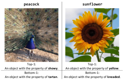
We use CLIP to compute the cosine similarity of an image and this text prompt (): “An object with the property of [MASK]”, where the [MASK] token is replaced with a candidate property . The score for each property is the mean similarity between the sentence prompt and all images collected for a noun:
| (5) |
This score serves to rank the candidate properties according to their relevance for a specific noun. Figure 2 shows the most and least relevant properties for the nouns peacock and sunflower.
3.3.3 Concreteness Ensemble Model (CEM)
The concreteness score for a property guides CEM towards “trusting” the language or the vision model more. We propose two CEM flavors which we describe as CEM-Pred and CEM-Gold. CEM-Pred uses the score () that is proposed by our concreteness prediction model for every candidate property , while CEM-Gold uses the score for in the Brysbaert et al. (2014) dataset.888Properties in Memory Colors have the highest average concreteness scores (0.82), followed by properties in Feature Norms (0.64) and Concept Properties (0.62). If there is no gold score for a property, we use the score of the word with the longest matching subsequence in the dataset.999This heuristic only applies to 15 (out of 209) properties in the Feature Norms dataset, and to 49 (out of 400) properties in Concept Properties-test. All 11 properties in Memory Colors have a gold concreteness value. The idea behind this heuristic is that properties without ground truth concreteness scores often have inflected forms or derivations in the dataset (e.g., sharpened/sharpen, invented/invention, etc.).101010It might happen that this heuristic matches antonymous words. Note that although these words have different meaning, they often have similar concreteness values (e.g., “happy”: 2.56, “unhappy”: 2.04; “moral”: 1.69, “immoral”: 1.59). We also experimented with GloVe word embedding cosine similarity which resulted in suboptimal performance (cf. Section 4). Additionally, sequence matching is much faster than GloVe similarity (cf. Appendix B).
Both CEMs combine the rank111111The rank of a property with respect to a model denoted as is defined as the index of property in the list of all properties sorted by decreasing . of proposed by the language model () and by CLIP () through a weighted sum which is controlled by the concreteness score, :
| (6) |
3.3.4 Concreteness Prediction Model
We generate concreteness scores using the model of Charbonnier and Wartena (2019) with FastText embeddings Bojanowski et al. (2017).
| Model | Prompt Selected |
| BERT | Most [NOUN-plural] are [MASK]. |
| RoBERTa | A/An [NOUN-singular] is generally [MASK]. |
| GPT-2 | Most [NOUN-plural] are [MASK]. |
| ViLT | [NOUN-plural] are [MASK]. |
| CLIP | An object with the property of [MASK]. |
The model leverages part-of-speech and suffix features to predict concreteness in a classical regression setting. We train the model on the 40k concreteness dataset Brysbaert et al. (2014), excluding the 425 adjectives found in our test sets. The model obtains a high Spearman correlation of 0.76 with the ground truth scores of the adjectives in our test sets. This result shows that automatically predicted scores are a viable alternative which allows the application of the method to new data and domains where hand-crafted resources might be unavailable.
3.3.5 Baselines
We compare the predictions of the language, vision, and ensemble models to the predictions of three baseline methods.
Random: Generates a Random property ranking for each noun.
GloVE: Ranking based on the cosine similarity of the GloVE embeddings Pennington et al. (2014) of the noun and the property.
Google Ngram: Ranking by the bigram frequency of each noun-property pair in Google Ngrams Brants and Franz (2009). If a noun-property pair does not appear in the corpus, we assign to it a frequency of 0.
3.4 Evaluation Metrics
We evaluate the property ranking proposed by each model using the top-K Accuracy (A@K), top-K recall (R@K), and Mean Reciprocal Rank (MRR) metrics. A@K is defined as the percentage of nouns for which at least one ground truth property is among the top-K predictions (Ettinger, 2020). R@K shows the proportion of ground truth properties retrieved in the top-K predictions. We report the average R@K across all nouns in a test set. MRR stands for the ground truth properties’ average reciprocal ranks (more precisely, the inverse of the rank, ). For all three metrics, high scores are better.
| Model | # Param | Img | Feature Norms | Concept Properties-test | Memory Colors | ||||||||||
| A@1 | A@5 | R@5 | R@10 | MRR | A@1 | A@5 | R@5 | R@10 | MRR | A@1 | A@2 | A@3 | |||
| Random | 0 | ✗ | 1.0 | 2.4 | 0.7 | 1.4 | .018 | 0.2 | 3.8 | 0.5 | 1.7 | .014 | 11.9 | 20.2 | 25.7 |
| GloVe | 0 | ✗ | 16.3 | 42.2 | 16.4 | 26.6 | .124 | 18.5 | 46.6 | 9.5 | 16.4 | .078 | 28.4 | 45.0 | 60.1 |
| Google-Ngram | 0 | ✗ | 23.4 | 65.2 | 31.5 | 47.7 | .192 | 27.9 | 72.1 | 18.5 | 30.3 | .122 | 44.0 | 63.3 | 69.7 |
| BERT-large | 345M | ✗ | 27.3 | 60.3 | 29.4 | 43.6 | .194 | 31.4 | 72.1 | 18.2 | 29.2 | .123 | 44.0 | 57.8 | 67.9 |
| RoBERTa-large | 354M | ✗ | 24.6 | 63.1 | 30.2 | 46.3 | .188 | 34.1 | 79.1 | 22.4 | 34.8 | .138 | 48.6 | 61.5 | 67.9 |
| GPT2-large | 1.5B | ✗ | 22.0 | 60.7 | 28.4 | 42.9 | .173 | 35.6 | 77.0 | 21.0 | 32.4 | .136 | 44.0 | 57.8 | 67.9 |
| GPT3-davinci | 175B | ✗ | 37.9 | 61.5 | 31.8 | 44.2 | - | 47.0 | 72.2 | 20.1 | 29.7 | - | 74.3 | 82.6 | 84.4 |
| ViLT | 135M | ✓ | 27.9 | 56.0 | 26.2 | 40.1 | .185 | 34.5 | 63.2 | 15.7 | 23.7 | .118 | 74.3 | - | - |
| CLIP-ViT/L14 | 427M | ✓ | 28.5 | 61.7 | 29.4 | 42.7 | .197 | 29.2 | 63.0 | 15.0 | 24.9 | .113 | 84.4 | 91.7 | 97.2 |
| CEM-Gold (GloVe) | 781M | ✓ | 38.9 | 75.6 | 39.4 | 53.3 | .249 | 48.6 | 84.8 | 27.0 | 39.3 | .171 | 83.5 | 92.7 | 99.1 |
| CEM-Gold | 781M | ✓ | 40.1 | 76.2 | 40.0 | 53.3 | .252 | 48.5 | 84.2 | 26.8 | 38.8 | .170 | 83.5 | 92.7 | 99.1 |
| CEM-Pred | 781M | ✓ | 39.9 | 75.8 | 40.0 | 52.5 | .251 | 49.9 | 85.8 | 28.1 | 40.0 | .175 | 88.1 | 96.3 | 99.1 |
3.5 Implementation Details
Prompt Selection We evaluate the performance of BERT-large, RoBERTa-large, GPT-2-large, and ViLT on the dev set (cf. Section 3.2) using the prompt templates proposed by Apidianaki and Garí Soler (2021). For CLIP, we handcraft a set of prompts that are close to the format that was recommended in the original paper Radford et al. (2021) and evaluate their performance on the dev set. We choose the prompt that yields the highest performance in terms of MRR on the dev set for each model, and use it for all our experiments (cf. Appendix A for details). Table 2 lists the prompt templates selected for each model.
Image Collection We collect images for the nouns in our datasets using the Bing Image Search API, an image query interface widely used for research purposes Kiela et al. (2016); Mostafazadeh et al. (2016).121212We use the bing-image-downloader API. We use again the dev set to determine the number of images needed for each noun. We find that good performance can be achieved with only ten images (cf. Figure 7 in Appendix C.1). Adding more images increases the computations needed without significantly improving the performance. Therefore, we set the number of images per noun to ten for all vision models and experiments.
Model Implementation All LMs and MLMs are built on the huggingface API.131313https://huggingface.co The CLIP model is adapted from the official repository.141414https://github.com/openai/CLIP CEM ensembles the RoBERTa-large and the CLIP-ViT/L14 models. The experiments were run on Quadro RTX 6000 24GB. All our experiments involve zero-shot and one-shot (for GPT-3) probing, hence no training of the models is needed. The inference time of CEM is naturally longer than that of individual models, but it is still very fast and only takes a few minutes for each dataset, with pre-computed image features. For more details on runtime refer to Section B, and specifically to Table 10, in the Appendix.
| Noun | Property | |
| most concrete | least concrete | |
| dandelion | yellow | annoying |
| cougar | brown | vicious |
| wand | round | magical |
| spear | sharp | dangerous |
| pyramid | triangular | mysterious |
4 Evaluation
4.1 Property Ranking Task
Table 3 shows the results obtained by the LMs, the MLMs and our CEM model on the Feature Norms, Concept Properties-test151515Contains all nouns in Concept Properties except from the ones in the Concept Properties-dev set. and Memory Colors datasets. The two flavors of CEM (CEM-Pred and CEM-Gold) outperform all other models with a significant margin across datasets. Interestingly, CEM-Pred performs better than CEM-Gold on the Concept Properties-test dataset. This may be due to the fact that 49 properties in this dataset do not have ground truth concreteness scores (vs. only 15 properties in Feature Norms), indicating that the prediction model probably approximates concreteness better in these cases, contributing to higher scores for CEM-Pred.
As explained in Section 3.3.3, we explore two different heuristics to select the score for these properties for CEM-Gold: longest matching subsequence and GloVE cosine similarity. The latter similarity metric results to a drop in performance on Feature Norms and almost identical performance for Concept-Properties-test.161616Specifically, for A@1 we observe a drop of 1.2 in Feature Norms and a gain of .1 for Concept Properties
We notice that the Google-Ngram baseline performs well on Feature Norms with results on par or superior to big LMs. The somewhat lower results obtained on Concept Properties-test might be due to the higher number of properties in this dataset (cf. Table 1), which makes the ranking task more challenging.171717The mean number of properties per noun in Concept Properties is 6.6, and 3.1 in Feature Norms.
There is also a higher number of noun-property pairs that are not found in Google Bigrams which are assigned a zero score.181818 26% of the pairs in Concept Properties vs. 15% for Feature Norms.
The Memory Colors dataset associates each noun with a single color so we only report Accuracy at top-K (last three columns of Table 3). We can compare these scores to a previous baseline, the top-1 Accuracy reported by Norlund et al. (2021) for the CLIP-BERT model which is 78.5.191919We cannot calculate the other scores because CLIP-BERT has not been made available. In this model, a CLIP encoded image is appended to BERT’s tokenized input before fine-tuning with a masked language modeling objective on 4.7M captions paired with 2.9M images. For more details refer to Norlund et al. (2021).
CEM-Pred and Gold both do better on this dataset (88.1). GPT-3 gets much higher scores than the other three language models on this task with a top-1 Accuracy of 74.3, but is outperformed by CLIP and CEM. Note that MRR does not apply to GPT-3 since it generates properties instead of reranking them (cf. Appendix A.3).
The multimodal model with the lowest performance, ViLT, is as good as GPT-3. CLIP falls halfway between ViLT and CEM-Pred/Gold. CEM-Pred and CEM-Gold present a clear advantage compared to language and multimodal models, achieving a top-1 Accuracy of 88.1. Although RoBERTa gets very low Accuracy on Memory Colors, it does not hurt performance when combined with CLIP in our CEM-Gold model. This is because the color properties in this dataset have high concreteness scores (0.82 on average), so CEM-Gold relies mainly on CLIP which works very well in this setting. CEM-Gold makes the same top-1 predictions as CLIP for 95 nouns (out of 109), while only 50 nouns are assigned the same color by CEM-Gold and RoBERTa.
4.2 Additional Analysis
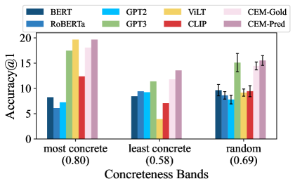
Concreteness level. We examine the performance of each model for properties at different concreteness levels. From the properties available for a noun in Feature Norms,202020In this experiment, we use 411 nouns (out of 509) from Feature Norms which have at least two properties. we keep a single property as our ground truth for this experiment: (a) most concrete: the property with the highest concreteness score in the Brysbaert et al. (2014) lexicon; (b) least concrete: the property with the lowest concreteness score; (c) random: a randomly selected property.212121We report the mean and standard deviation on 10 trials. Figure 3 shows the top-1 Accuracy of the models for the properties in each concreteness band. Examples of nouns with their most and least concrete properties are given in Table 4. The results of this experiment confirm our initial assumption that MLMs (e.g., CLIP and ViLT) are better at capturing concrete properties, and LMs (e.g., RoBERTa and GPT-2) are better at identifying abstract ones. GPT-3 is the only LM that performs better for concrete than for abstract properties, while still falling behind CEM variations.
| Noun | Model | Top-3 Properties |
| swan | RoBERTa | male, white, black |
![[Uncaptioned image]](https://cdn.awesomepapers.org/papers/79b15335-9e38-4f64-90a1-e61403b7d590/swan.jpg) |
CLIP | white, graceful, gentle |
| GPT-3 | graceful, regal, stately | |
| CEM-Gold | white, large, graceful | |
| CEM-Pred | white, endangered, graceful | |
| ox | RoBERTa | male, white, black |
![[Uncaptioned image]](https://cdn.awesomepapers.org/papers/79b15335-9e38-4f64-90a1-e61403b7d590/ox.jpg) |
CLIP | endangered, wild, harvested |
| GPT-3 | strong, muscular, brawny | |
| CEM-Gold | large, wild, friendly | |
| CEM-Pred | large, wild, hairy | |
| plum | RBTa | edible, yellow, red |
| CLIP | purple, edible, picked | |
| CEM | edible, purple, harvested | |
| GPT-3 | tart, acidic, sweet | |
| orange | RoBERTa | edible, yellow, orange |
![[Uncaptioned image]](https://cdn.awesomepapers.org/papers/79b15335-9e38-4f64-90a1-e61403b7d590/orange.jpg) |
CLIP | orange, citrus, juicy |
| GPT-3 | tart, acidic, sweet | |
| CEM-Gold | orange, edible, healthy | |
| CEM-Pred | orange,edible,citrus | |
| cape | RoBERTa | black, white, fashionable |
![[Uncaptioned image]](https://cdn.awesomepapers.org/papers/79b15335-9e38-4f64-90a1-e61403b7d590/cape.jpg) |
CLIP | cozy, dressy, cold |
| GPT-3 | tart, acidic, sweet | |
| CEM-Gold | fashionable, dark, grey | |
| CEM-Pred | fashionable,grey,dark | |
Rank Improvement.
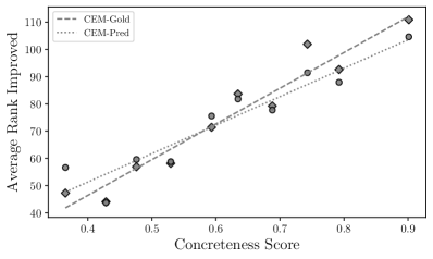
We investigate the relationship between the performance of CEM and the concreteness score of the properties in Concept Properties-test. We measure the rank improvement (RI) for a property () that occurs when using CEM compared to when RoBERTa is used as follows:
| (7) |
A high RI score for means that its rank is improved with CEM compared to RoBERTa. We calculate the RI for properties at different concreteness levels. We sort the 400 properties in Concept Properties-test by increasing the concreteness score and group them into ten bins of 40 properties each. We find a clear positive relationship between the average RI and concreteness scores within each bin, as shown in Figure 4. This confirms that both CEM-Pred and CEM-Gold perform better with concrete properties.
Ensemble Weight Selection.
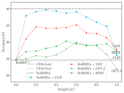
We explore whether a dynamic concreteness-based ensemble weight outperforms a fixed one. We experiment with different model combinations (RoBERTa with BERT, GPT-2, and ViLT) with an interpolation weight that takes values in the range [0,1]. If the weight is close to 0, CEM relies more on RoBERTa; if it is 1, CEM relies more on the second model.
| (8) |
We also run the best performing RoBERTa + CLIP combination again using weights fixed in this way, i.e. without recourse to the properties’ concreteness score as in CEM-Pred and in CEM-Gold. Note that we do not expect the combination of two text-based LMs to improve Accuracy a lot compared to RoBERTa alone. Our intuition is confirmed by the results obtained on Feature Norms and shown in Figure 5.
The dashed and dotted straight lines in the figure represent the top-1 Accuracy of CEM-Gold and CEM-Pred, respectively, when the weights used are not the ones on the x-axis, but the gold and predicted concreteness scores (cf. Equation 6). To further highlight the importance of concreteness in interpolating the models, we provide additional results and comparisons in Appendix D.2. Note that CEM-Gold and CEM-Pred have highly similar performance and actual output.
On average over all nouns, they propose 4.35 identical properties at top-5 for nouns in Feature Norms, and 4.41 for nouns in Concept Properties-test.
We observe a slight improvement in top-1 Accuracy (5%) when ensembling two text-based LMs (RoBERTa + BERT or RoBERTa + GPT-2). Text-based LMs have similar output distributions, hence combining them does not change the final distribution much. The RoBERTa + ViLT ensemble model achieves higher performance due to the interpolation with an image-based model, but it does not reach the Accuracy of the CEM models (RoBERTa + CLIP). The ViLT model gets lower performance than CLIP when combined with RoBERTa, because it was exposed to much less data than CLIP during training (400M vs. 30M). Finally, we notice that the best performance of RoBERTa + CLIP with fixed weight is slightly lower than that of the CEM models. This indicates that using a fixed weight to ensemble two models hurts performance compared to calibrating their mutual contribution using the concreteness score. Another advantage of the concreteness score is that it is more transferable since it does not require tuning on new datasets.
Properties Quality.
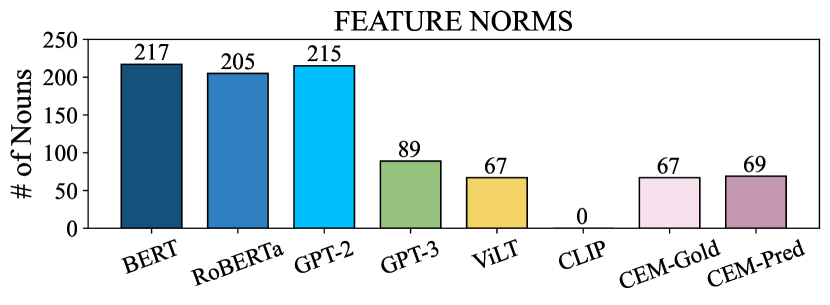
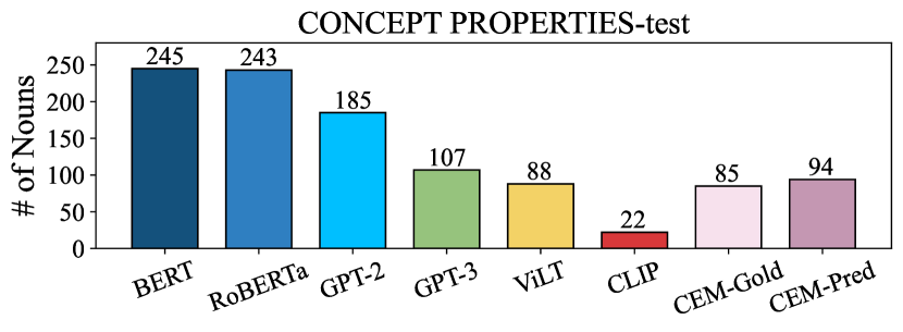
Table 5 shows a random sample of the top-3 predictions made by each model for nouns in Concept Properties-test. We notice that the properties proposed by the two flavors of CEM are both perceptual and abstract, due to their access to both a language and a vision model. We further observe that CEM retrieves rarer and more varied properties for different nouns, compared to the language models. 222222Details on the frequency of the properties retrieved by each model are reported in Appendix E.1. We provide more randomly sampled qualitative examples in Appendix E.5.
Figure 6 shows the number of nouns for which a model made the exact same top-3 predictions.232323Refer to E.3 for the number of nouns with exact same top-K predictions for different values of K. For example GPT-3 proposed the properties [tart, acidic, sweet, juicy, smooth] for 20 different nouns242424apple, plum, grapefruit, tangerine, orange, lime, lemon, grape, rhubarb, cherry, cap, cape, blueberry, strawberry, pine, pineapple, prune, raspberry, nectarine, cranberry in the same order. Note that better prompt engineering might decrease the number of repeated properties. However, we are already prompting GPT-3 with one shot, whereas the other models, including CEM are zero-shot. RoBERTa predicted [male, healthy, white, black, small] for both mittens and penguin, and [male, black, white, brown, healthy] for owl and flamingo. We observe that CEM-Pred and CEM-Gold are less likely to retrieve the same top-K predictions for a noun than language models. CEM combines the variability and accuracy of CLIP with the benefits of text-based models, which are exposed to large volumes of texts during pre-training.
5 Conclusion
We propose a new ensemble model for noun property prediction which leverages the strengths of language models and multimodal (vision) models.
Our model, CEM, calibrates the contribution of the two types of models in a property ranking task by relying on the properties’ concreteness level. The results show that the CEM model, which combines RoBERTa and CLIP outperforms powerful text-based language models (such as GPT-3) with significant margins in three evaluation datasets. Additionally, our methodology yields better performance than alternative ensembling techniques, confirming our hypothesis that concrete properties are more accessible through images, and abstract properties through text. The Accuracy scores obtained on the larger datasets
show that there is still room for improvement for this challenging task.
6 Limitations
Our experiments address concreteness at the lexical level, specifically using scores assigned to adjectives in an external resource Brysbaert et al. (2014) or predicted using Charbonnier and Wartena (2019). Another option would be to use the concreteness of the noun phrases formed by the adjectives and the nouns they modify. We would expect this to be different than the concreteness of adjectives in isolation since the concreteness of the nouns would have an impact on that of the resulting phrase
(e.g., useful knife vs. useful idea). We were not able to evaluate the impact of noun phrase concreteness on property prediction because the property datasets used in our experiments mostly contain concrete nouns. Another limitation of our methodology is the reliance on pairing images with nouns. In particular, we use a search engine to retrieve images corresponding to nouns in order to get grounded predictions from the vision model. Finally, we only evaluate our methodology in English and leave experimenting with other languages to future work, since this would require the collection of multi-lingual semantic association datasets and/or the translation of existing ones. We did not pursue this extension for this paper as Multilingual Clip model weights only became available very recently.
7 Acknowledgements
We thank Marco Baroni for his feedback on an earlier version of the paper. This research is based upon work supported in part by the DARPA KAIROS Program (contract FA8750-19-2-1004), the DARPA LwLL Program (contract FA8750-19-2-0201), the IARPA BETTER Program (contract 2019-19051600004), and the NSF (Award 1928631). Approved for Public Release, Distribution Unlimited. The views and conclusions contained herein are those of the authors and should not be interpreted as necessarily representing the official policies, either expressed or implied, of DARPA, IARPA, NSF, or the U.S. Government.
References
- Aghajanyan et al. (2021) Armen Aghajanyan, Anchit Gupta, Akshat Shrivastava, Xilun Chen, Luke Zettlemoyer, and Sonal Gupta. 2021. Muppet: Massive Multi-task Representations with Pre-Finetuning. In Proceedings of the 2021 Conference on Empirical Methods in Natural Language Processing, pages 5799–5811.
- Alayrac et al. (2022) Jean-Baptiste Alayrac, Jeff Donahue, Pauline Luc, Antoine Miech, Iain Barr, Yana Hasson, Karel Lenc, Arthur Mensch, Katie Millican, Malcolm Reynolds, et al. 2022. Flamingo: a visual language model for few-shot learning. arXiv preprint arXiv:2204.14198.
- Apidianaki and Garí Soler (2021) Marianna Apidianaki and Aina Garí Soler. 2021. ALL dolphins are intelligent and SOME are friendly: Probing BERT for nouns’ semantic properties and their prototypicality. In Proceedings of the Fourth BlackboxNLP Workshop on Analyzing and Interpreting Neural Networks for NLP, pages 79–94, Punta Cana, Dominican Republic. Association for Computational Linguistics.
- Barnard and Johnson (2005) Kobus Barnard and Matthew Johnson. 2005. Word sense disambiguation with pictures. Artificial Intelligence, 167(1-2):13–30.
- Barsalou and Wiemer-Hastings (2005) Lawrence W. Barsalou and Katja Wiemer-Hastings. 2005. Situating abstract concepts. pages 129–163.
- Bojanowski et al. (2017) Piotr Bojanowski, Edouard Grave, Armand Joulin, and Tomas Mikolov. 2017. Enriching word vectors with subword information. Transactions of the Association for Computational Linguistics, 5:135–146.
- Bouraoui et al. (2020) Zied Bouraoui, José Camacho-Collados, and Steven Schockaert. 2020. Inducing Relational Knowledge from BERT. In The Thirty-Fourth AAAI Conference on Artificial Intelligence, pages 7456–7463, New York, NY, USA. AAAI Press.
- Brants and Franz (2009) Thorsten Brants and Alex Franz. 2009. Web 1T 5-gram, 10 European languages version 1. Linguistic Data Consortium, Philadelphia.
- Bruni et al. (2012) Elia Bruni, Gemma Boleda, Marco Baroni, and Nam-Khanh Tran. 2012. Distributional semantics in technicolor. In Proceedings of the 50th Annual Meeting of the Association for Computational Linguistics (Volume 1: Long Papers), pages 136–145, Jeju Island, Korea. Association for Computational Linguistics.
- Bruni et al. (2014) Elia Bruni, Nam Khanh Tran, and Marco Baroni. 2014. Multimodal Distributional Semantics. J. Artif. Int. Res., 49(1):1–47.
- Brysbaert et al. (2014) Marc Brysbaert, Amy Beth Warriner, and Victor Kuperman. 2014. Concreteness ratings for 40 thousand generally known english word lemmas. Behavior research methods, 46(3):904–911.
- Byrne (1974) Brian Byrne. 1974. Item concreteness vs spatial organization as predictors of visual imagery. Memory & Cognition, 2(1):53–59.
- Charbonnier and Wartena (2019) Jean Charbonnier and Christian Wartena. 2019. Predicting word concreteness and imagery. In Proceedings of the 13th International Conference on Computational Semantics-Long Papers, pages 176–187. Association for Computational Linguistics.
- Devereux et al. (2014) Barry J Devereux, Lorraine K Tyler, Jeroen Geertzen, and Billi Randall. 2014. The Centre for Speech, Language and the Brain (CSLB) concept property norms. Behavior research methods, 46(4):1119–1127.
- Devlin et al. (2019) Jacob Devlin, Ming-Wei Chang, Kenton Lee, and Kristina Toutanova. 2019. BERT: Pre-training of deep bidirectional transformers for language understanding. In Proceedings of the 2019 Conference of the North American Chapter of the Association for Computational Linguistics: Human Language Technologies, Volume 1 (Long and Short Papers), pages 4171–4186, Minneapolis, Minnesota. Association for Computational Linguistics.
- Ettinger (2020) Allyson Ettinger. 2020. What BERT is not: Lessons from a new suite of psycholinguistic diagnostics for language models. Transactions of the Association for Computational Linguistics, 8:34–48.
- Friendly et al. (1982) Michael Friendly, Patricia E Franklin, David Hoffman, and David C Rubin. 1982. The Toronto Word Pool: Norms for imagery, concreteness, orthographic variables, and grammatical usage for 1,080 words. Behavior Research Methods & Instrumentation, 14(4):375–399.
- Gordon and Van Durme (2013) Jonathan Gordon and Benjamin Van Durme. 2013. Reporting Bias and Knowledge Acquisition. In Proceedings of the 2013 Workshop on Automated Knowledge Base Construction, AKBC ’13, page 25–30, New York, NY, USA. Association for Computing Machinery.
- Herbelot and Vecchi (2015) Aurélie Herbelot and Eva Maria Vecchi. 2015. Building a shared world: Mapping distributional to model-theoretic semantic spaces. In Proceedings of the 2015 Conference on Empirical Methods in Natural Language Processing, pages 22–32.
- Hewitt et al. (2018) John Hewitt, Daphne Ippolito, Brendan Callahan, Reno Kriz, Derry Tanti Wijaya, and Chris Callison-Burch. 2018. Learning translations via images with a massively multilingual image dataset. In Proceedings of the 56th Annual Meeting of the Association for Computational Linguistics (Volume 1: Long Papers), pages 2566–2576, Melbourne, Australia. Association for Computational Linguistics.
- Kiela et al. (2014) Douwe Kiela, Felix Hill, Anna Korhonen, and Stephen Clark. 2014. Improving multi-modal representations using image dispersion: Why less is sometimes more. In Proceedings of the 52nd Annual Meeting of the Association for Computational Linguistics (Volume 2: Short Papers), pages 835–841, Baltimore, Maryland. Association for Computational Linguistics.
- Kiela et al. (2016) Douwe Kiela, Anita Lilla Verő, and Stephen Clark. 2016. Comparing data sources and architectures for deep visual representation learning in semantics. In Proceedings of the 2016 Conference on Empirical Methods in Natural Language Processing, pages 447–456, Austin, Texas. Association for Computational Linguistics.
- Kim et al. (2021) Wonjae Kim, Bokyung Son, and Ildoo Kim. 2021. Vilt: Vision-and-language transformer without convolution or region supervision. In International Conference on Machine Learning, pages 5583–5594. PMLR.
- Kiros et al. (2018) Jamie Kiros, William Chan, and Geoffrey Hinton. 2018. Illustrative language understanding: Large-scale visual grounding with image search. In Proceedings of the 56th Annual Meeting of the Association for Computational Linguistics (Volume 1: Long Papers), pages 922–933.
- Lazaridou et al. (2015) Angeliki Lazaridou, Nghia The Pham, and Marco Baroni. 2015. Combining language and vision with a multimodal skip-gram model. In Proceedings of the 2015 Conference of the North American Chapter of the Association for Computational Linguistics: Human Language Technologies, pages 153–163, Denver, Colorado. Association for Computational Linguistics.
- Lazaridou et al. (2016) Angeliki Lazaridou, Nghia The Pham, and Marco Baroni. 2016. The red one!: On learning to refer to things based on discriminative properties. In Proceedings of the 54th Annual Meeting of the Association for Computational Linguistics (Volume 2: Short Papers), pages 213–218, Berlin, Germany. Association for Computational Linguistics.
- Li et al. (2019) Liunian Harold Li, Mark Yatskar, Da Yin, Cho-Jui Hsieh, and Kai-Wei Chang. 2019. Visualbert: A simple and performant baseline for vision and language. arXiv preprint arXiv:1908.03557.
- Liu et al. (2019) Yinhan Liu, Myle Ott, Naman Goyal, Jingfei Du, Mandar Joshi, Danqi Chen, Omer Levy, Mike Lewis, Luke Zettlemoyer, and Veselin Stoyanov. 2019. Roberta: A robustly optimized bert pretraining approach. arXiv preprint arXiv:1907.11692.
- Lu et al. (2019) Jiasen Lu, Dhruv Batra, Devi Parikh, and Stefan Lee. 2019. Vilbert: Pretraining task-agnostic visiolinguistic representations for vision-and-language tasks. Advances in neural information processing systems, 32.
- McRae et al. (2005) Ken McRae, George S Cree, Mark S Seidenberg, and Chris McNorgan. 2005. Semantic feature production norms for a large set of living and nonliving things. Behavior research methods, 37(4):547–559.
- Mikolov et al. (2018) Tomas Mikolov, Edouard Grave, Piotr Bojanowski, Christian Puhrsch, and Armand Joulin. 2018. Advances in Pre-Training Distributed Word Representations. In Proceedings of the International Conference on Language Resources and Evaluation (LREC 2018).
- Mostafazadeh et al. (2016) Nasrin Mostafazadeh, Ishan Misra, Jacob Devlin, Margaret Mitchell, Xiaodong He, and Lucy Vanderwende. 2016. Generating natural questions about an image. In Proceedings of the 54th Annual Meeting of the Association for Computational Linguistics (Volume 1: Long Papers), pages 1802–1813, Berlin, Germany. Association for Computational Linguistics.
- Norlund et al. (2021) Tobias Norlund, Lovisa Hagström, and Richard Johansson. 2021. Transferring knowledge from vision to language: How to achieve it and how to measure it? In Proceedings of the Fourth BlackboxNLP Workshop on Analyzing and Interpreting Neural Networks for NLP, pages 149–162, Punta Cana, Dominican Republic. Association for Computational Linguistics.
- Paik et al. (2021) Cory Paik, Stéphane Aroca-Ouellette, Alessandro Roncone, and Katharina Kann. 2021. The World of an Octopus: How Reporting Bias Influences a Language Model’s Perception of Color. In Proceedings of the 2021 Conference on Empirical Methods in Natural Language Processing, pages 823–835, Online and Punta Cana, Dominican Republic. Association for Computational Linguistics.
- Paivio et al. (1968) Allan Paivio, John C Yuille, and Stephen A Madigan. 1968. Concreteness, imagery, and meaningfulness values for 925 nouns. Journal of experimental psychology, 76(1p2):1.
- Pennington et al. (2014) Jeffrey Pennington, Richard Socher, and Christopher D Manning. 2014. Glove: Global vectors for word representation. In Proceedings of the 2014 conference on empirical methods in natural language processing (EMNLP), pages 1532–1543.
- Petroni et al. (2019) Fabio Petroni, Tim Rocktäschel, Sebastian Riedel, Patrick Lewis, Anton Bakhtin, Yuxiang Wu, and Alexander Miller. 2019. Language models as knowledge bases? In Proceedings of the 2019 Conference on Empirical Methods in Natural Language Processing and the 9th International Joint Conference on Natural Language Processing (EMNLP-IJCNLP), pages 2463–2473, Hong Kong, China. Association for Computational Linguistics.
- Radford et al. (2021) Alec Radford, Jong Wook Kim, Chris Hallacy, Aditya Ramesh, Gabriel Goh, Sandhini Agarwal, Girish Sastry, Amanda Askell, Pamela Mishkin, Jack Clark, et al. 2021. Learning transferable visual models from natural language supervision. In International Conference on Machine Learning, pages 8748–8763. PMLR.
- Radford et al. (2019) Alec Radford, Jeffrey Wu, Rewon Child, David Luan, Dario Amodei, Ilya Sutskever, et al. 2019. Language models are unsupervised multitask learners. OpenAI blog, 1(8):9.
- Sharma et al. (2018) Piyush Sharma, Nan Ding, Sebastian Goodman, and Radu Soricut. 2018. Conceptual captions: A cleaned, hypernymed, image alt-text dataset for automatic image captioning. In Proceedings of the 56th Annual Meeting of the Association for Computational Linguistics (Volume 1: Long Papers), pages 2556–2565.
- Shwartz and Choi (2020) Vered Shwartz and Yejin Choi. 2020. Do neural language models overcome reporting bias? In Proceedings of the 28th International Conference on Computational Linguistics, pages 6863–6870, Barcelona, Spain (Online). International Committee on Computational Linguistics.
- Silberer et al. (2013) Carina Silberer, Vittorio Ferrari, and Mirella Lapata. 2013. Models of semantic representation with visual attributes. In Proceedings of the 51st Annual Meeting of the Association for Computational Linguistics (Volume 1: Long Papers), pages 572–582, Sofia, Bulgaria. Association for Computational Linguistics.
- Song et al. (2022) Haoyu Song, Li Dong, Weinan Zhang, Ting Liu, and Furu Wei. 2022. CLIP Models are Few-Shot Learners: Empirical Studies on VQA and Visual Entailment. In Proceedings of the 60th Annual Meeting of the Association for Computational Linguistics (Volume 1: Long Papers), pages 6088–6100.
- Su et al. (2022) Yixuan Su, Tian Lan, Yahui Liu, Fangyu Liu, Dani Yogatama, Yan Wang, Lingpeng Kong, and Nigel Collier. 2022. Language Models Can See: Plugging Visual Controls in Text Generation. arXiv preprint arXiv:2205.02655.
- Takase and Kiyono (2021) Sho Takase and Shun Kiyono. 2021. Lessons on parameter sharing across layers in transformers. arXiv preprint arXiv:2104.06022.
- Tan and Bansal (2019) Hao Tan and Mohit Bansal. 2019. LXMERT: Learning Cross-Modality Encoder Representations from Transformers. In Proceedings of the 2019 Conference on Empirical Methods in Natural Language Processing and the 9th International Joint Conference on Natural Language Processing (EMNLP-IJCNLP), pages 5100–5111.
- Tsimpoukelli et al. (2021) Maria Tsimpoukelli, Jacob L Menick, Serkan Cabi, SM Eslami, Oriol Vinyals, and Felix Hill. 2021. Multimodal few-shot learning with frozen language models. Advances in Neural Information Processing Systems, 34:200–212.
- Vaswani et al. (2017) Ashish Vaswani, Noam Shazeer, Niki Parmar, Jakob Uszkoreit, Llion Jones, Aidan N Gomez, Łukasz Kaiser, and Illia Polosukhin. 2017. Attention is all you need. Advances in neural information processing systems, 30.
- Wu et al. (2016) Yonghui Wu, Mike Schuster, Zhifeng Chen, Quoc V. Le, Mohammad Norouzi, Wolfgang Macherey, Maxim Krikun, Yuan Cao, Qin Gao, Klaus Macherey, Jeff Klingner, Apurva Shah, Melvin Johnson, Xiaobing Liu, Łukasz Kaiser, Stephan Gouws, Yoshikiyo Kato, Taku Kudo, Hideto Kazawa, Keith Stevens, George Kurian, Nishant Patil, Wei Wang, Cliff Young, Jason Smith, Jason Riesa, Alex Rudnick, Oriol Vinyals, Greg Corrado, Macduff Hughes, and Jeffrey Dean. 2016. Google’s Neural Machine Translation System: Bridging the Gap between Human and Machine Translation. arXiv preprint:1609.08144.
- Yamada et al. (2020) Ikuya Yamada, Akari Asai, Hiroyuki Shindo, Hideaki Takeda, and Yuji Matsumoto. 2020. LUKE: Deep Contextualized Entity Representations with Entity-aware Self-attention. In Proceedings of the 2020 Conference on Empirical Methods in Natural Language Processing (EMNLP), pages 6442–6454.
- Yang et al. (2021a) Yue Yang, Joongwon Kim, Artemis Panagopoulou, Mark Yatskar, and Chris Callison-Burch. 2021a. Induce, edit, retrieve: Language grounded multimodal schema for instructional video retrieval. arXiv preprint arXiv:2111.09276.
- Yang et al. (2021b) Yue Yang, Artemis Panagopoulou, Qing Lyu, Li Zhang, Mark Yatskar, and Chris Callison-Burch. 2021b. Visual goal-step inference using wikihow. In Proceedings of the 2021 Conference on Empirical Methods in Natural Language Processing, pages 2167–2179.
- Yun et al. (2021) Tian Yun, Chen Sun, and Ellie Pavlick. 2021. Does vision-and-language pretraining improve lexical grounding? In Findings of the Association for Computational Linguistics: EMNLP 2021, pages 4357–4366, Punta Cana, Dominican Republic. Association for Computational Linguistics.
- Zhang et al. (2022) Chenyu Zhang, Benjamin Van Durme, Zhuowan Li, and Elias Stengel-Eskin. 2022. Visual commonsense in pretrained unimodal and multimodal models. arXiv preprint arXiv:2205.01850.
- Zhang et al. (2021) Lisai Zhang, Qingcai Chen, Joanna Siebert, and Buzhou Tang. 2021. Semi-supervised Visual Feature Integration for Language Models through Sentence Visualization. In Proceedings of the 2021 International Conference on Multimodal Interaction, pages 682–686.
Appendix A Prompt Selection
A.1 Language Model Prompts
In our experiments with language models, we use the 11 prompts proposed by Apidianaki and Garí Soler (2021) for retrieving noun properties. As shown in Table 6, these involve nouns in singular and plural forms. The performance achieved by each language model with these prompts on the Concept Properties development set is given in Table 8. The results show that model performance varies significantly with different prompts. The best-performing prompt is different for each model. For BERT and GPT-2, the “most + PLURAL” obtains the highest Recall and MRR scores. The best performing prompt for RoBERTa-large is “SINGULAR + generally”, and “PLURAL” for ViLT.
| Prompt Type | Prompt Example |
| SINGULAR | a motorcycle is [MASK]. |
| PLURAL | motorcycles are [MASK]. |
| SINGULAR + usually | a motorcycle is usually [MASK]. |
| PLURAL + usually | motorcycles are usually [MASK]. |
| SINGULAR + generally | a motorcycle is generally [MASK]. |
| PLURAL + generally | motorcycles are generally [MASK]. |
| SINGULAR + can be | a motorcycle can be [MASK]. |
| PLURAL + can be | motorcycles can be [MASK]. |
| most + PLURAL | most motorcycles are [MASK]. |
| all + PLURAL | all motorcycles are [MASK]. |
| some + PLURAL | some motorcycles are [MASK]. |
A.2 CLIP Prompts
For CLIP, we handcraft ten prompts and report their performance on the Concept Properties development set in Table 7. Similar to what we observed with language models, CLIP performance is also sensitive to the prompts used. We select for our experiments the prompt “An object with the property of [MASK].”, which obtains the highest average Accuracy and MRR score on the Concept Properties development set.
| Prompt Type | Acc@1 | R@5 | R@10 | MRR |
| [MASK] | 26.0 | 13.1 | 21.9 | .097 |
| This is [MASK]. | 28.0 | 9.6 | 13.6 | .089 |
| A [MASK] object. | 22.0 | 13.2 | 18.9 | .089 |
| This is a [MASK] object. | 22.0 | 12.0 | 17.2 | .087 |
| The item is [MASK]. | 18.0 | 7.5 | 17.2 | .074 |
| The object is [MASK]. | 24.0 | 10.5 | 16.2 | .088 |
| The main object is [MASK]. | 24.0 | 10.3 | 20.3 | .091 |
| An object which is [MASK]. | 28.0 | 13.7 | 19.9 | .106 |
| An object with the property of [MASK]. | 32.0 | 12.3 | 20.0 | .108 |
| Prompt Type | BERT-large | RoBERTa-large | GPT-2-large | ViLT | ||||||||
| R@5 | R@10 | MRR | R@5 | R@10 | MRR | R@5 | R@10 | MRR | R@5 | R@10 | MRR | |
| SINGULAR | 8.9 | 17.3 | .067 | 17.1 | 23.6 | .092 | 14.0 | 27.5 | .097 | 12.6 | 18.2 | .085 |
| PLURAL | 11.5 | 21.9 | .070 | 10.5 | 21.1 | .085 | 14.9 | 23.7 | .098 | 15.5 | 24.5 | .105 |
| SINGULAR + usually | 12.7 | 24.5 | .082 | 15.5 | 26.5 | .098 | 16.2 | 25.3 | .107 | 11.8 | 18.7 | .088 |
| PLURAL + usually | 14.4 | 27.6 | .107 | 13.3 | 23.7 | .106 | 17.8 | 24.6 | .113 | 15.6 | 21.7 | .091 |
| SINGULAR + generally | 14.3 | 23.6 | .087 | 17.7 | 27.9 | .119 | 18.7 | 29.2 | .114 | 12.7 | 19.4 | .083 |
| PLURAL + generally | 15.0 | 26.7 | .097 | 16.0 | 25.3 | .105 | 17.4 | 26.7 | .128 | 9.8 | 18.6 | .075 |
| SINGULAR + can be | 12.4 | 23.9 | .102 | 14.7 | 22.7 | .090 | 14.3 | 24.7 | .105 | 9.2 | 14.1 | .056 |
| PLURAL + can be | 16.0 | 26.4 | .107 | 12.1 | 17.7 | .073 | 10.2 | 18.3 | .096 | 10.0 | 14.2 | .060 |
| most + PLURAL | 16.7 | 27.3 | .107 | 12.6 | 25.7 | .098 | 20.0 | 33.4 | .122 | 12.6 | 20.8 | .095 |
| all + PLURAL | 13.4 | 20.5 | .083 | 8.2 | 13.5 | .073 | 19.6 | 31.3 | .113 | 14.4 | 20.4 | .103 |
| some + PLURAL | 11.2 | 21.5 | .082 | 16.4 | 23.5 | .100 | 15.4 | 31.5 | .097 | 10.7 | 17.2 | .091 |
| Feature Norms | Concept Properties-test | Memory Colors | |||||||||
| Acc@1 | R@5 | R@10 | MRR | Acc@1 | R@5 | R@10 | MRR | Acc@1 | Acc@3 | Acc@5 | |
| CLIP-ViT/B32 | 24.8 | 24.8 | 36.1 | .172 | 27.6 | 13.0 | 19.6 | .097 | 83.5 | 95.4 | 99.1 |
| CLIP-ViT/B16 | 25.3 | 27.4 | 38.9 | .184 | 28.3 | 14.3 | 22.0 | .103 | 87.2 | 96.3 | 98.2 |
| CLIP-ViT/L14 | 26.1 | 29.2 | 43.3 | .192 | 29.2 | 15.0 | 24.9 | .113 | 82.6 | 96.3 | 99.1 |
A.3 GPT-3 Prompts
Since we do not have complete control of GPT-3 at this moment, we treat GPT-3 as a question-answering model using the following prompt in a one-shot example setting:
Use ten adjectives to describe
the properties of kiwi:\n
1. tart\n2. acidic\n3. sweet\n
4. juicy\n5. smooth\n6. fuzzy\n
7. green\n8. brown\n9. small\n
10. round\n
Use ten adjectives to describe
the properties of [NOUN]:\n
We use the text-davinci-001 engine of GPT-3 which costs $0.06 per 1,000 tokens. On average, it costs $0.007 to generate 10 properties for each noun.
Appendix B Inference Times
Table 10 provides details about the runtime of the experiments. The second column of the Table indicates whether a model uses images. Training the concreteness predictor for CEM-Pred takes 10 minutes. Inference for all nouns in the datasets with CEM-Pred only takes a couple of seconds. Note that CEM-Pred is faster than CEM-Gold, since CEM-Gold leverages the longest matching subsequence heuristic (LMS) or GloVe vector cosine similarity in order to find the concreteness score of the most similar word in Brysbaert et al. (2014) for properties without a gold concreteness score. The times reported in the table for image feature pre-computation correspond to the time needed for computing embeddings for 200 images for each noun in a dataset, which is only computed once for each dataset. We, however, only use 10 of them for the final CEM models (cf. Appendix C.1).
| Feature Norms | Concept Properties-test | Memory Colors | |||||||||||
| Model | Img | Time |
|
Time |
|
Time |
|
||||||
| GloVe | ✗ | 11 sec. | - | 12 sec. | - | 10 sec. | - | ||||||
| Google Ngram | ✗ | 15 min. | - | 15 min. | - | 15 min. | - | ||||||
| BERT-large | ✗ | 3 min. 18 sec. | - | 7 min 33 sec. | - | 4 sec. | - | ||||||
| RoBERTa-large | ✗ | 2 min. 31 sec. | - | 5 min 50 sec | - | 3 sec. | - | ||||||
| GPT2-large | ✗ | 48 min. 2 sec. | - | 1 hr. 39 min. | - | 38 sec. | - | ||||||
| GPT3-davinci | ✗ | 6 min. 50 sec. | - | 8 min 7 sec | - | 1 min. 27 sec. | - | ||||||
| ViLT | ✓ | 1 hr. 40 min. | 2 hr. 50 min. | 2 hr. 45 min. | 3 hr. 20 min. | 57 sec. | 33 min. | ||||||
| CLIP-ViLT/L14 | ✓ | 52 seconds | 5 hr. 40 min. | 2 min. 10 sec. | 6 hr. 41 min. | 13 sec. | 1 hr. 13 min | ||||||
| CEM-gold (GloVE) | ✓ | 4 min. 14 sec. | 5 hr. 40 min. | 10 min. 4 sec. | 6 hr. 41 min. | 28 sec. | 1 hr. 13 min | ||||||
| CEM-gold (LMS) | ✓ | 3 min. 30 sec. | 5 hr. 40 min. | 8 min. 12 sec. | 6 hr. 41 min. | 20 sec. | 1 hr. 13 min | ||||||
| CEM-pred | ✓ | 4 min. 29 sec. | 5 hr. 40 min. | 7 min. 20 sec. | 6 hr. 41 min. | 49 sec. | 1 hr. 13 min | ||||||
Appendix C Implementation of CLIP
C.1 Number of Images
For each noun, we collected 200 images from Bing. Given that it is not practical to use such a high number of images for a large-scale experiment, we investigate the performance of CLIP with different number of images. We first filter the 200 images collected for each noun to remove duplicates. We then sort the remaining images based on the cosine similarity of each image with the sentence “A photo of [NOUN].”.
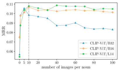
We pick the top-M images and gradually increase the value of M.252525When M = 0, we use the CLIP text encoder to encode the noun as the image embedding. Figure 7 shows the MRR obtained by CLIP on the Concept Properties development set with a varying number of images. We observe that the model’s MRR score increases with a higher number of images. Nevertheless, the improvement is marginal when the number of images is higher than ten and starts to overfit when the number is higher than 20. Therefore, we decided to use ten images for all experiments involving CLIP.
C.2 CLIP Size
We evaluate three sizes of CLIP, from small to large: CLIP-ViT/B16, CLIP-ViT/B32, and CLIP-ViT/L14. As shown in Figure 7, the performance positively correlates with the model size. The largest model, CLIP-ViT/L14 has a higher MRR score than the other two models. We also report the performance of the three CLIP models on Feature Norms, Concept Properties-test, and Memory Colors in Table 9, indicating that the larger CLIP model yields better performance across metrics.
| Model | Images | Non-Prototypical | Prototypical | ||||||||
| Acc@5 | Acc@10 | R@5 | R@10 | MRR | Acc@5 | Acc@10 | R@5 | R@10 | MRR | ||
| Random | ✗ | 4.13 | 7.67 | 2.73 | 4.96 | 0.030 | 4.66 | 8.03 | 2.15 | 3.84 | 0.025 |
| GloVe | ✗ | 22.59 | 33.20 | 16.99 | 26.76 | 0.124 | 30.05 | 44.56 | 15.68 | 26.71 | 0.124 |
| Google-Ngram | ✗ | 45.19 | 57.96 | 39.22 | 58.80 | 0.240 | 39.64 | 56.99 | 24.06 | 36.47 | 0.142 |
| BERT-large | ✗ | 35.76 | 51.28 | 30.22 | 48.12 | 0.197 | 45.60 | 58.81 | 28.16 | 39.42 | 0.191 |
| RoBERTa-large | ✗ | 35.76 | 48.92 | 28.53 | 46.39 | 0.176 | 47.67 | 63.73 | 28.95 | 43.08 | 0.200 |
| GPT2-large | ✗ | 36.35 | 48.92 | 29.92 | 45.79 | 0.181 | 40.93 | 55.96 | 24.12 | 37.23 | 0.166 |
| GPT3-davinci | ✗ | 30.84 | 40.67 | 25.77 | 39.42 | - | 55.18 | 64.51 | 38.30 | 49.66 | - |
| ViLT | ✓ | 34.97 | 46.76 | 28.85 | 42.70 | 0.211 | 38.34 | 53.63 | 23.52 | 36.57 | 0.159 |
| CLIP-ViT/L14 | ✓ | 32.22 | 43.81 | 25.08 | 37.95 | 0.159 | 52.59 | 69.95 | 33.67 | 49.82 | 0.226 |
| CEM-Gold (Ours) | ✓ | 41.85 | 54.03 | 35.88 | 49.55 | 0.217 | 64.77 | 75.39 | 43.11 | 56.06 | 0.289 |
| CEM-Pred (Ours) | ✓ | 41.65 | 51.47 | 35.11 | 46.46 | 0.211 | 65.80 | 74.87 | 44.67 | 56.20 | 0.306 |
| Feature Norms | Concept Properties-test | Memory Colors | |||||||||
| Acc@1 | R@5 | R@10 | MRR | Acc@1 | R@5 | R@10 | MRR | Acc@1 | Acc@3 | Acc@5 | |
| CEM-Gold | 40.1 | 40.5 | 53.3 | .252 | 48.3 | 26.9 | 39.1 | .171 | 82.6 | 96.3 | 99.1 |
| CEM-Pred | 39.9 | 40.4 | 52.5 | .251 | 49.9 | 28.1 | 40.0 | .175 | 84.4 | 97.2 | 99.1 |
| CEM-random | 35.4 | 38.3 | 51.0 | .232 | 46.3 | 25.3 | 36.5 | .162 | 62.4 | 90.8 | 94.5 |
| CEM-average | 38.7 | 41.0 | 53.0 | .249 | 48.3 | 28.0 | 40.2 | .173 | 71.6 | 92.7 | 99.1 |
| CEM-max | 36.9 | 38.4 | 51.3 | .238 | 48.6 | 26.7 | 38.1 | .167 | 67.0 | 90.8 | 96.3 |
| CEM-min | 25.1 | 34.2 | 50.1 | .204 | 30.1 | 21.2 | 34.1 | .135 | 69.7 | 95.4 | 98.2 |
Appendix D CEM Variations
D.1 Concretess Prediction Model
In Table 12, we report the results obtained by the CEM model using predicted concreteness values (instead of gold standard ones). We predict these values by training the model of Charbonnier and Wartena (2019) using the concreteness scores of 40k words (all parts-of-speech) in the Brysbaert et al. (2014) dataset. We exclude 425 adjectives that are found in the Feature Norms, Concept Properties, and Memory Colors datasets.262626In total, the three datasets contain 487 distinct properties (adjectives). The concreteness prediction model uses FastText embeddings Mikolov et al. (2018) enhanced with POS and suffix features. We evaluate the model on the 425 adjectives that were left out during training and for which we have ground truth scores. The Spearman correlation between the predicted and gold scores is 0.76, showing that our automatically predicted scores can be safely used in our ensemble model instead of the gold standard ones.
D.2 CEM Weight Selection
We also experiment with different ways for generating scores and combining the property ranks proposed by the models. (a) CEM-pred:We generate a concreteness score using the model of Charbonnier and Wartena (2019) and FastText embeddings Bojanowski et al. (2017). We train the model on the 40k concreteness dataset Brysbaert et al. (2014), excluding the 425 adjectives found in our evaluation datasets. The model obtains a high Spearman correlation of 0.76 against the ground truth scores of the adjectives in our test sets, showing that automatically predicted scores are a good alternative to manually defined ones. (b) CEM-random: We randomly generate a score for each property and use it to combine the ranks from two models. (c) CEM-average: We use the average of the property ranks; (d) CEM-high: We use the maximum rank of the property; (e) CEM-low: We use the minimum rank of the property. Table 12 shows the comparison between CEM-Pred, CEM-Gold and models that rely on these alternative weight generation and ensembling methods on Feature Norms. CEM achieves the highest performance across all metrics, indicating that concreteness offers a reliable criterion for model ensembling under unsupervised scenarios.
Appendix E Qualitative Analysis
E.1 Unigram Prediction Frequency
In Table 13, we report the mean Google unigram frequency Brants and Franz (2009) for all properties in the top 5 predictions of each model. We observe that our CEM model – which achieves the best performance among the tested models, as shown in Table 3 – often predicts medium-frequency words. This is a desirable property of our model compared to models which would instead predict highly frequent or rare words (highly specific or technical terms).
This is the case for GPT3 and CLIP, which propose rarer attributes but obtain lower performance than CEM. It is worth noting that, contrary to CLIP, GPT3 retrieves properties from an open vocabulary.
Given that Google NGrams frequencies are computed based on text, many common properties might not be reported. For example, Feature Norms propose as typical attributes of an “ambulance”: loud, white, fast, red, large, orange. The frequency of the corresponding property-noun bigrams (e.g., loud ambulance, white ambulance) are: 0, 687, 50, 193, 283, and 0. Meanwhile, the bigrams formed with less typical properties (e.g., old, efficient, modern, and independent) have a higher frequency (1725, 294, 314, and 457). While language models rely on text and, thus, suffer from reporting bias, vision-based models can retrieve properties that are rarely stated in the text.
| Model | Concept Properties-test | Feature Norms | ||
| Unigram Freq. | Bigram Freq. | Unigram Freq. | Bigram Freq. | |
| BERT | 53M | 11.6K | 55M | 7.6K |
| RoBERTa | 50M | 6.8K | 53M | 6K |
| GPT-2 | 96M | 10.3K | 78M | 6.4K |
| GPT-3 | 24M | 6.5K | 25M | 2.8K |
| ViLT | 50M | 6.2K | 40M | 3.8K |
| CLIP | 11M | 5.3K | 18M | 2.2K |
| CEM-Gold | 32M | 7.4K | 33M | 4.1K |
| CEM-Pred | 34M | 7.1K | 31M | 6.1K |
E.2 Prototypical Property Retrieval
We carry out an additional experiment aimed at estimating the performance of the models on prototypical vs. non-prototypical properties. Prototypical properties are the ones that apply to most of the objects in the class denoted by the noun (e.g., red strawberries); in contrast, non-prototypical properties describe attributes of a smaller subset of the objects denoted by the noun (e.g., delicious strawberry). We make the assumption that prototypical properties are common and, often, visual or perceptual; we expect them to be more rarely stated in texts and, hence, harder to retrieve using language models than using images.
We use the split of the Feature Norms dataset performed by Apidianaki and Garí Soler (2021) into prototypical and non-prototypical properties, based on the quantifier annotations found in the Herbelot and Vecchi (2015) dataset.272727Three native English speakers were asked to rate properties in Feature Norms based on how often they describe a noun, by choosing a label among [NO, FEW, SOME, MOST, ALL]. The first split (Prototypical) contains 785 prototypical adjective-noun pairs (for 386 nouns) annotated with at least two all labels, or with a combination of all and most (healthy banana [all-all-all]). The second set (Non-Prototypical) contains 807 adjective-noun pairs (for 509 nouns) with adjectives in the ground truth that are not included in the Prototypical set. In Table 11, we report the performance of each model in retrieving these properties. In the ALL, MOST column we consider properties that have at least 2 ALL annotations, with the combination of a MOST annotation, and in the SOME column, we consider all properties that do not contain NO and FEW annotations, and have at least one SOME annotation. The results confirm our intuition that non-prototypical properties are more frequently mentioned in the text. This is reflected in the score of the Google NGram baseline for these properties. For prototypical properties, our CEM model outperforms all other models.
E.3 Same Top-K Predictions by Different Nouns
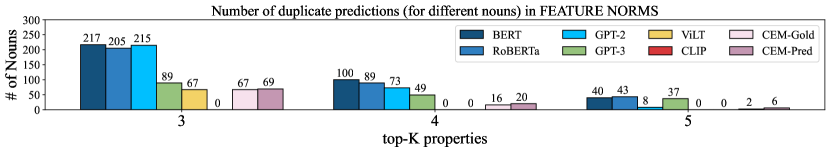
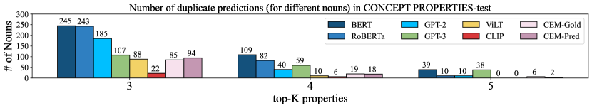
Figure 8 shows the number of nouns in the Feature Norms and Concept Properties-test datasets for which a model made the exact same top-K predictions. We observe that LMs consistently repeat the same properties for different nouns, while MLMs exhibit a higher variation in their predictions.
E.4 Multi-piece Performance
| Model | Feature Norms | |||||
| # Multi-piece Properties | Acc@5 | Acc@10 | R@5 | R@10 | MRR | |
| BERT-large | 106 | 0.0 | 0.0 | 0.0 | 0.0 | 0.009 |
| RoBERTa-large | 590 | 23.77 | 32.02 | 22.64 | 32.27 | 0.182 |
| GPT2-large | 12 | 0.0 | 0.0 | 0.0 | 0.0 | 0.018 |
| GPT3-davinci | 0 | - | - | - | - | - |
| ViLT | 106 | 1.57 | 2.55 | 7.51 | 13.0 | 0.060 |
| CLIP-ViT/L14 | 45 | 4.72 | 5.50 | 55.95 | 66.67 | 0.401 |
| CEM-Gold (Ours) | 590/45 | 36.54/1.2 | 43.81/3.14 | 37.65/13.10 | 49.59/35.71 | 0.245/0.124 |
| CEM-Pred (Ours) | 590/45 | 32.22/1.77 | 41.85/3.73 | 33.7/20.24 | 46.76/42.86 | 0.165/0.122 |
| Model | Concept Properties-test | |||||
| # Multi-piece Properties | Acc@5 | Acc@10 | R@5 | R@10 | MRR | |
| BERT-large | 429 | 0.0 | 0.33 | 0.0 | 0.59 | 0.006 |
| RoBERTa-large | 1939 | 45.42 | 59.56 | 19.12 | 27.65 | 0.120 |
| GPT2-large | 60 | 0.0 | 0.0 | 0.0 | 0.0 | 0.010 |
| GPT3-davinci | 27 | 0.33 | 0.50 | 7.41 | 11.11 | - |
| ViLT | 429 | 1.66 | 3.99 | 2.43 | 5.77 | 0.029 |
| CLIP-ViT/L14 | 300 | 16.47 | 20.13 | 39.12 | 49.12 | 0.029 |
| CEM-Gold (Ours) | 1939/300 | 54.58/6.49 | 68.39/9.65 | 26.24/13.03 | 38.92/20.96 | 0.161/0.095 |
| CEM-Pred (Ours) | 1939/300 | 56.99/5.63 | 69.87/9.62 | 27.31/12.12 | 39.35/21.05 | 0.165/0.078 |
Each model splits words into a different number of word pieces. Table 14 shows the number of multi-piece properties for each model, and its performance on these properties. We observe that all models perform worse than average (refer to Table 3 for the average performance) on the multi-piece properties, however, CEM has the smallest reduction in performance compared to the average values. This could be because CEM relies on information from two models with different tokenizers.
E.5 Qualitative Examples
Table 15 contains more examples of the top-5 predictions for nouns in Concept Properties-test and Feature Norms.
| Noun | Image | Model | Top-5 Properties |
| wand | ![[Uncaptioned image]](https://cdn.awesomepapers.org/papers/79b15335-9e38-4f64-90a1-e61403b7d590/wand.jpg) |
RBTa | necessary,useful,unnecessary,white,small |
| CLIP | magical,magic,cunning,fizzy,extendable | ||
| GPT-3 | long,thin,flexible,smooth,light | ||
| CEM-Gold | magical,long,brown,magic,adjustable | ||
| CEM-Pred | magical,brown,magic,long,golden | ||
| horse | ![[Uncaptioned image]](https://cdn.awesomepapers.org/papers/79b15335-9e38-4f64-90a1-e61403b7d590/horse.jpg) |
RBTa | healthy,white,black,stable,friendly |
| CLIP | stable,majestic,fair,free,wild | ||
| GPT-3 | strong,fast,powerful,muscular,big | ||
| CEM-Gold | stable,friendly,free,wild,healthy | ||
| CEM-Pred | stable,friendly,free,wild,healthy | ||
| raven | ![[Uncaptioned image]](https://cdn.awesomepapers.org/papers/79b15335-9e38-4f64-90a1-e61403b7d590/raven.jpg) |
RBTa | black,white,harmless,aggressive,solitary |
| CLIP | unlucky,nocturnal,dark,solitary,cunning | ||
| GPT-3 | black,glossy,sleek,shiny,intelligent | ||
| CEM-Gold | solitary,black,dark,harmless,rare | ||
| CEM-Pred | solitary,black,dark,harmless,rare | ||
| surfboard | ![[Uncaptioned image]](https://cdn.awesomepapers.org/papers/79b15335-9e38-4f64-90a1-e61403b7d590/surfboard.jpg) |
RBTa | expensive,white,comfortable,small,waterproof |
| CLIP | paddled,overfished,aerodynamic,concave,beachwear | ||
| GPT-3 | hard,smooth,slick,colorful,long | ||
| CEM-Gold | waterproof,paddled,beachwear,long,cool | ||
| CEM-Pred | waterproof,long,cheap,cool,durable | ||
| limousine | RBTa | expensive,black,white,empty,large | |
| CLIP | luxurious,decadent,ostentatious,expensive,showy | ||
| GPT-3 | long,sleek,spacious,luxurious,comfortable | ||
| CEM-Gold | expensive,luxurious,large,long,comfortable | ||
| CEM-Pred | expensive,luxurious,large,long,comfortable | ||
| violin | ![[Uncaptioned image]](https://cdn.awesomepapers.org/papers/79b15335-9e38-4f64-90a1-e61403b7d590/violin.jpg) |
RBTa | expensive,white,small,black,electric |
| CLIP | acoustic,fiddly,strummed,traditional,rhythmic | ||
| GPT-3 | wooden,long,thin,stringed,musical | ||
| CEM-Gold | acoustic,fiddly,small,cheap,unique | ||
| CEM-Pred | acoustic,small,unique,cheap,brown | ||
| barn | RBTa | large,white,small,red,common | |
| CLIP | old-fashioned,run-down,harvested,red,old | ||
| GPT-3 | old,large,red,wooden,rusty | ||
| CEM-Gold | red,large,old,spacious,portable | ||
| CEM-Pred | red,old,spacious,large,rectangular | ||
| oak | RBTa | healthy,white,green,tall,harvested | |
| CLIP | green,sticky,edible,large,harvested | ||
| GPT-3 | strong,sturdy,hard,dense,heavy | ||
| CEM-Gold | green,harvested,large,edible,brown | ||
| CEM-Pred | green,harvested,large,edible,brown | ||
| radish | ![[Uncaptioned image]](https://cdn.awesomepapers.org/papers/79b15335-9e38-4f64-90a1-e61403b7d590/radish.jpg) |
RBTa | edible,poisonous,delicious,white,small |
| CLIP | edible,nutritious,healthy,harvested,young | ||
| GPT-3 | crunchy,peppery,spicy,earthy,pungent | ||
| CEM-Gold | edible,healthy,harvested,delicious,white | ||
| CEM-Pred | edible,white,harvested,healthy,delicious | ||
| toilet | ![[Uncaptioned image]](https://cdn.awesomepapers.org/papers/79b15335-9e38-4f64-90a1-e61403b7d590/toilet.jpg) |
RBTa | portable,dirty,open,common,small |
| CLIP | sinkable,brown,emptied,round,short | ||
| GPT-3 | dirty,smelly,clogged,rusty,filthy | ||
| CEM-Gold | large,white,small,brown,sinkable | ||
| CEM-Pred | portable,white,uncomfortable,waterproof,dirty | ||
| bluejay | ![[Uncaptioned image]](https://cdn.awesomepapers.org/papers/79b15335-9e38-4f64-90a1-e61403b7d590/bluejay.jpg) |
RBTa | male,black,small,healthy,white |
| CLIP | blue,gentle,crunchy,wild,friendly | ||
| GPT-3 | blue,small,blue,blue,blue | ||
| CEM-Gold | blue,friendly,edible,small,endangered | ||
| CEM-Pred | blue,endangered,small,friendly,wild | ||
| donkey | ![[Uncaptioned image]](https://cdn.awesomepapers.org/papers/79b15335-9e38-4f64-90a1-e61403b7d590/donkey.jpg) |
RBTa | black,male,white,healthy,brown |
| CLIP | humorous,annoying,short,brown,darned | ||
| GPT-3 | stubborn,strong,sure-footed,intelligent,social | ||
| CEM-Gold | brown,grey,large,short,slow | ||
| CEM-Pred | brown,large,slow,hairy,friendly |