Visualizing Attractors of the Three-Dimensional Generalized Hénon Map
Abstract
We study dynamics of a generic quadratic diffeomorphism, a 3D generalization of the planar Hénon map. Focusing on the dissipative, orientation preserving case, we give a comprehensive parameter study of codimension-one and two bifurcations. Periodic orbits, born at resonant, Neimark-Sacker bifurcations, give rise to Arnold tongues in parameter space. Aperiodic attractors include invariant circles and chaotic orbits; these are distinguished by rotation number and Lyapunov exponents. Chaotic orbits include Hénon-like and Lorenz-like attractors, which can arise from period-doubling cascades, and those born from the destruction of invariant circles. The latter lie on paraboloids near the local unstable manifold of a fixed point.
Since Hénon’s observation of strange, chaotic attractors in his eponymous two-dimensional map,Hénon (1976) this quadratic map has become a pivotal model to understand chaotic dynamics in the plane, see Refs. [Guckenheimer and Holmes, 2002; Kuznetsov, 2004]. It is of much interest to understand the dynamics of higher-dimensional generalizations of this map as models for the onset and development of chaotic dynamics. As a prototypical model, we study the so-called 3D generalized Hénon map,Gonchenko et al. (2005) which is a quadratic normal form for several bifurcation scenarios. Extending upon previous work, we study the periodic and aperiodic dynamics of this map using a variety of visualizations in both parameter and phase space. For example, Arnold tongues, or resonant regions, in parameter space correspond to attracting periodic orbits in phase space. We compute heteroclinic trajectories between orbits in the tongues as well as in period-doubling cascades. We also follow the evolution of invariant circles as they bifurcate, some of which can become complex chaotic attractors.
I Introduction
The two-dimensional Hénon mapHénon (1976) is the quadratic diffeomorphism of the plane: every such diffeomorphism is conjugate to a map in the two-parameter Hénon family. Prominent rigorous results for this diffeomorphism include that of Devaney and Nitecki, Devaney and Nitecki (1979) who showed that the dynamics of its bounded orbits are conjugate to a Smale horseshoe in some parameter regimes, and that of Benedicks and Carleson,Benedicks and Carleson (1991) who showed that when the Jacobian is sufficiently small there are cases for which the map has a transitive attractor with a positive Lyapunov exponent. It was also shown that the horseshoe in this map can be thought of as arising from an anti-integrable limit, where the dynamics becomes non-deterministic.Sterling and Meiss (1998)
Some of these results have been generalized to higher-dimensional maps. For the three-dimensional (3D) case it was shown in Ref. [Lomelí and Meiss, 1998] that every quadratic diffeomorphism with a quadratic inverse is conjugate to the map
| (1) | ||||
This analysis was later generalized to include 3D quadratic diffeomorphisms that have quartic inverses, Elhadj and Sprott (2009) and to higher dimensions. Lenz, Lomelí, and Meiss (1999) The diffeomorphism (1) arises as a normal from in the volume preserving () case near a fixed point with three unit multipliers.Dullin and Meiss (2008, 2009) It has also been shown to be a normal form near a map with a saddle-focus fixed point that has a quadratic homoclinic tangency. Gonchenko et al. (2005); Gonchenko, Meiss, and Ovsyannikov (2006) The theory of anti-integrability also applies to these maps when , see e.g., Ref. [Hampton and Meiss, 2022].
The map has seven parameters, six in the quadratic polynomial and , the Jacobian determinant. This parameter set can be reduced, as noted in Ref. [Lomelí and Meiss, 1998]: whenever and ,***If one of these is violated, other scaling transformations can be found to eliminate two of the parameters. an affine coordinate transformation allows one to set
| (2) |
Using this simplification, (1) depends only on and the Jacobian .
The case has been called “the 3D Hénon map” since it only has one nonlinear term, similar to the classical Hénon map.Hénon (1976) In a series of papers starting with Refs. [Gonchenko et al., 2005; Gonchenko, Meiss, and Ovsyannikov, 2006], Gonchenko and collaborators focus on the formation of chaotic attractors for this map.††† In their notation . These attractors are shown to be “wild hyperbolic”‡‡‡Nearby maps have Newhouse tangencies between its stable and unstable manifolds. Turaev and Shilnikov (1998) near the parameters , where a pair of fixed points are born with multipliers . These attractors are also “pseudo-hyperbolic,”§§§Its tangent space splits into a a strong stable subspace and a complementary subspace that exponentially expands volume. like the Lorenz attractor, implying that every orbit in the attractor has at least one positive and one negative Lyapunov exponent. According to Ref. [Gonchenko and Gonchenko, 2016], there are five types of such attractors formed from the unstable manifold of a fixed point, including “Lorenz-like” and several “figure-eight” attractors.Gonchenko, Simo, and Vieiro (2013) Moreover, there are infinite cascades in parameter space of nearby systems with Lorenz-like attractors.Gonchenko and I. (2017) Chaotic attractors for the non-orientable case have also been studied.Gonchenko et al. (2021a)
Following Gonchenko et al., we will primarily study the 3D Hénon case using the scaling (2) and taking , so that the map is volume contracting and orientation preserving. We focus on two examples:
-
(SC)
Strongly Contracting: ,
-
(MC)
Moderately Contacting: ,
allowing to vary. In §II, we recall basic bifurcation behavior of periodic orbits for a 3D map using the trace and second trace of the Jacobian. These bifurcation conditions are transformed to conditions on for the fixed points of (1) in §III. Similar bifurcation criterion were obtained for the 3D Hénon map in Ref. [Zhao et al., 2017] for the case that , as well as in Ref. [Richter, 2002] when for three and more dimensions. In §IV, we prove that all bounded orbits of the 3D Hénon map lie within a finite cube about origin, following the proof of a related theorem in Ref. [Lomelí and Meiss, 1998].
The simplest bounded orbits are stable and periodic. Parameter regions in the -plane containing such attractors, analogous to Arnold tongues, are computed in §V, where we also compute heteroclinic manifolds between stable and unstable orbits. In §VI, we study aperiodic attractors, computing the maximal Lyapunov exponent to distinguish between regular and chaotic cases. Regular aperiodic attractors come in the form of invariant circles, which we study in §VI.1 extending the volume-preserving case studied in Ref. [Dullin and Meiss, 2009]. In §VI.2, we find Hénon-like attractors for case (SC) and discrete, Lorenz-like attractorsGonchenko et al. (2021b) for case (MC). Additionally, we observe chaotic attractors arising from bifurcations of invariant circles that are unlike those in Refs. [Gonchenko et al., 2014; Gonchenko, Gonchenko, and Turaev, 2021]; these also do not seem to be related to the generalizations of Smale’s horseshoe to 3D found by Ref. [Zhang, 2016].
II Bifurcations for 3D Maps
For a fixed point of a 3D map , the eigenvalues of the Jacobian are given by the characteristic polynomial
| (3) |
We refer to these as the multipliers of the fixed point. Here is the trace and . An expression for the “second trace”, , can be obtained from the Cayley-Hamilton theorem: a matrix satisfies its own characteristic polynomial, . Multiplying this by implies that . Finally, multiplying the Cayley polynomial by and taking the trace gives
| (4) |
Of course, the multipliers can be related to the coefficients of (3) by the symmetric polynomials,
| (5) | ||||
More generally, for an orbit, , that has period , , the Jacobian becomes
Thus, using the same process as above, we can find a general expression for the trace and second trace of a period- orbit:
Following Ref. [Kuznetsov and Meijer, 2019], the simplest, local codimension-one bifurcations—saddle-node, period-doubling and Neimark-Sacker—occur when at least one multiplier has unit modulus. Each of these occurs on a surface in , given in Table 1. Sections through these surfaces for four values of are shown in Fig. 1; similar figures can be found in Ref. [Lomelí and Meiss, 1998] for the case and in Ref. [Gonchenko and Gonchenko, 2016], where they are referred to as “saddle-charts.”
| CoD | Bifurcation | Multiplier | ||
| 1 | Saddle-Node | (SN) | ||
| Period Doubling | (PD) | |||
| Neimark-Sacker | (NS) | |||
| 2 | (R1) | |||
| (R2) | ||||
| (R3) | ||||
| (R4) | ||||
| Saddle-Node Flip | (SNf) | |||
Saddle-node (SN) bifurcations require a unit multiplier, so that (3) gives . This corresponds to a line in the -plane, shown in blue in Fig. 1. A period-doubling (PD) bifurcation occurs when there is a multiplier, or ; shown in red in Fig. 1. The third codimension-one bifurcation, the Neimark-Sacker (NS), occurs when there is a pair of complex multipliers with unit modulus; it generically results in the creation of an invariant circle or pair of periodic orbits with differing stabilities. Since , (5) gives , so that . The resulting line, , is shown in black in Fig. 1. Solving for the complex multipliers gives
| (6) |
or that , for rotation number .
Some codimension-two bifurcations occur along the NS line when , and generically result in the birth of a pair of period- orbits. The endpoints of the NS line occur where it intersects the SN and PD lines at and , labeled (R1) and (R2), respectively, in Table 1. The table also shows the period-three (R3) and period-four (R4) cases. Finally, the saddle-node flip (SNf) bifurcation point, with multipliers is at the intersection of the PD and SN lines.
A curve in parameter space along which there is a double multiplier, say , for , corresponds to the transition from real to complex multipliers. Using (5), this occurs when along the parametric curve
| (7) |
This curve has two branches when , one of which has a cusp at , i.e., at . When , this curve is tangent to the SN line and crosses the R1 point, and when the curve is tangent to the PD line and crosses the R2 point. Four segments of these curves, labelled by ranges of the double multiplier, are shown in Fig. 1.
We also include representative configurations of the multipliers in the complex plane relative to the unit circle for each region of the plane in Fig. 1. For , there exists a small triangular region with all stable multipliers () that is bounded by the SN, PD and NS lines with vertices R1, R2, and SNf. Otherwise, the SN and PD lines divide the plane into four regions where stability types of the multipliers of the fixed points alternate between having one unstable and two stable multipliers and two unstable and one stable multiplier.


III Fixed Points of the Quadratic Map
We now apply the results of §II to fixed points of (1) with parameter convention (2). The fixed points have the form where
| (8) | ||||
provided . These are born in a saddle-node bifurcation when with . Thinking of as a bifurcation parameter, the form (8) implies that there is a fixed point at , say, when whenever , or equivalently when
| (9) |
The stability of the fixed points is determined by the linearization of (1),
This is in companion form, implying that at a fixed point the trace and second trace are
| (10) |
and the Jacobian is .
The fixed points lie on a line in the -plane that can be found by eliminating and from (10),
| (11) |
and are born at the intersection of this line with the SN line from Table 1,
Moreover, (10) gives
Since , this implies that lies below and above the SN line in the plane. Therefore when , if there exists an attracting fixed point, it must be .
Using the equations for the SN and PD lines in Table 1, the fixed points are born above the PD line when , or
Provided , one of the fixed points undergoes a period-doubling bifurcation at
| (12) |
An expression for the period doubling value of is obtained from (9): . Note that for a fixed point to ‘double,’ it needs to exist, thus we must have . In addition, when , the fixed point doubles, and when , the point doubles.
Similarly, using (10) and the expression in Table 1 for the NS bifurcation gives
| (13) |
provided the denominator is nonzero. Of course, this bifurcation only exists if the fixed points intersect the NS line on the interval .Again, (9) can be used to determine the bifurcation value, .
When the parameters are fixed, the generic bifurcation diagrams of Fig. 1 can be transformed to corresponding diagrams for a fixed point in the plane; details are given in Appendix A, including criteria for codimension-two bifurcations. The results are shown in Fig. 2 for the fixed point —as this is the only fixed point that can be attracting—for cases (SC) and (MC).


IV Bounded Orbits
In Ref. [Lomelí and Meiss, 1998], it was shown that if the quadratic form is positive definite and , then there is a cube that contains all bounded orbits of (1); equivalently, all points outside of this cube escape to infinity. We show in this section that a similar argument can be used for the case , where is semi-definite, for any .
Lemma 1.
If , , and , then all bounded orbits of the map (1) are contained within the cube where
| (14) |
Proof.
For an orbit of the map (1), and , so the map is equivalent to the forward and backward difference equations
| (15) | ||||
| (16) |
There are three cases to consider that depend on which term in the sequence is largest.
-
1.
: then (15) gives
giving a lower bound to the forward iterate. Notice this inequality implies that the next iterate lies above an even, piecewise-parabolic curve with negative vertical intercept. Thus there exists such that whenever , we have
Here is the maximum root of , given by (14). This implies that . Recursively applying this argument to each forward step implies that
This is a monotone increasing sequence that cannot have a finite limit: if it were to converge, it would have to converge to one of the fixed points , (8), but this is impossible since, by simple calculation, .
-
2.
: then (16) gives
giving an upper bound to the preimage. This inequality is the space below an even, downward facing piecewise parabola with a positive vertical-intercept. As before, when ,
Applying this argument recursively implies that is a monotone decreasing sequence. Again, the sequence must be unbounded.
- 3.
Thus, bounded orbits of the map (1) with , and must lie within a -cube about origin. ∎
To illustrate this result, we compute the volume of bounded orbits, i.e. the volume of the basin of any attractors, for the cases (SC) and (MC), see Fig. 3. For each point on a grid in the -plane for which the fixed points (8) exist (), we choose initial conditions on a uniform grid in a cube with bounds (14) that vary with . An orbit is declared to be unbounded if it leaves the -cube within iterates.
The selected parameters in Fig. 3 focus on the triangular regions of Fig. 2 where is an attracting fixed point. The bifurcation curves (dashed) and codimension-two points are also shown (refer to the legend in Fig. 2). Note that near the SN line, the volume of bounded orbits in the -cube is small since most are found near the fixed points, which are close together.

V Periodic Attractors
In this section we compute regions in parameter space for which (1) has attracting periodic orbits. If there is a unique, bounded attractor, it can easily be found by choosing an appropriate initial condition within the cube of Lem. 1 and iterating until the orbit limits on the attractor. Once the transient is removed, parameter regions of periodic behavior can be computed by looking for recurrence.
Computed periodic regions are shown in Fig. 4 for the two cases, (SC) and (MC). To compute these, the initial point is set to when neither of the fixed points exist (i.e., to the right of the SN line in the -plane) or to , near the fixed point. For each on a grid, the map (1) is iterated times to eliminate transients. The orbit is declared to diverge (white region) if for some , where is the maximum of (14) over the studied parameter region ( for (SC) and for (MC)). Otherwise the point is iterated up to more steps, checking for return time, defined as the first time, , for which the distance
| (17) |
Thus we find approximately periodic orbits up to period ; the period is indicated by the color map in Fig. 4. If an orbit is not periodic by this definition, the point is colored black or gray; we will discuss the dynamics in these regions in §VI.

The number of transient iterations, recurrence tolerance, and grid size were chosen to provide sufficient detail at the pictured resolution but still lessen the computational expense.
Note that since this method uses a single initial condition, it cannot find cases where there are multiple attractors. Additionally, it is possible that the chosen initial condition leads to an unbounded orbit when there is still an attractor somewhere in the -cube. Nevertheless, for almost all points that have bounded orbits in Fig. 3, the orbit iterated in Fig. 4 is also bounded; therefore, with a few exceptions, it does not appear that the orbit of is unbounded when there are other bounded orbits. We plan to discuss such exceptional cases and the case of multiple attractors in future papers.
The largest, blue regions in Fig. 4 correspond to period-one, where is attracting. This region is bounded by the SN, PD, and NS curves seen in Fig. 2. When the fixed point loses stability at the PD curve an attracting period-two orbit is born; the period-two (vivid orange) region is prominent in Fig. 4(a), though there is also a thin period-two region just below the PD curve in Fig. 4(b). Period-doubling bifurcations leading to period-four (magenta) and eight (red) are also seen in Fig. 4(a). By contrast, in Fig. 4(b), the period-two orbit in (MC) looses stability by a NS bifurcation, so a doubling cascade is not seen in this case.
Resonant “tongues”, analogous to the Arnold tongues found in circle maps, start along the NS curve where is rational; these are prominent in Fig. 4(b). Especially visible are the (yellow), (magenta), (dark green), and (brown) tongues. Bifurcation points along the NS curve for the first two of these were indicated in Fig. 2 as R3 and R4.
Enlargements of case (SC), shown in Fig. 5, and of case (MC), Fig. 7, provide more detail. In the following two subsections, we show a few examples of the corresponding orbits in phase space for the period-doubling cascade and resonant tongues.

V.1 Period-Doubling Cascade
A supercritical period doubling bifurcation generically occurs when a real multiplier of an attracting periodic orbit passes through , the PD line of Fig. 1, and results in the creation of a stable orbit of twice the period. As is well known from studies of 1D maps, this behavior often recurs, resulting in a cascade of doubling bifurcations that accumulates leading to the formation of a chaotic attractor.Guckenheimer and Holmes (2002); Kuznetsov (2004) Such a cascade is prominent in case (SC) seen in Fig. 4(a) and its enlargement Fig. 5. Cascades are also often seen at the ends of the resonant tongues; most apparent for case (MC) in Fig. 7, which shows a multitude of tongues radiating from the attracting fixed point region.
To visualize the progression of the period-doubling cascade in case (SC), we fix along the line segment shown in Fig. 5 and vary . The four points (triangles) along this segment correspond to the parameters used to find the orbits seen in Fig. 6, which are pictured using triangles of the same color. Figure 6 also shows the heteroclinic orbit that lies on the unstable manifold of the fixed point (black triangle), to the attracting orbit. The unstable manifold of the fixed point is traced out by iterates of a set of initial conditions starting in a ball of radius 0.01 about . The first point, at , is a stable period-one orbit. It period doubles at , creating an attracting period-2 orbit, shown for (orange triangles). The unstable manifold of is also shown in orange. As continues to decrease the doubling recurs forming next a stable period-4 (magenta) and then a stable period-8 (red). The parameters for these are listed in Table 2.
Also prominent in Fig. 5 are a number of shrimps, common structures seen in two-parameter families of one Gallas (1994); MacKay and Tresser (1987) and two-dimensional maps. Façanha, Oldeman, and Glass (2013) Shrimps are prototypical structures formed by saddle-node bifurcations of periodic orbits in a ‘sea of chaos.’ These structures will not be discussed further in this paper.
| Case | Behavior | Color | |
| fixed point | black | ||
| doubling bifurcation | |||
| period-2 attractor | orange | ||
| quadrupling bifurcation | |||
| period-4 attractor | magenta | ||
| octupling bifurcation | |||
| period-8 attractor | red | ||
| period-3 attractor | yellow | ||
| period-4 attractor | magenta |

V.2 Resonant Tongues

At a resonant point, , on the NS curve, a pair of period orbits are born when . These period- orbits exist in a “tongue”-shaped region bounded by curves of SN bifurcations. While a pair of periodic orbits still exist for the strongly resonant cases, , the resonant regions can be more complexKuznetsov (2004). Near the NS curve of the fixed point, one of these orbits is stable and is easily detected by our recurrence algorithm. Such tongues are especially prominent in Fig. 7 for case (MC).
The pair of orbits found within the tongues can be used to find heteroclinic orbits from the period- saddle to its attracting counterpart. Examples for and 4 are seen for case (MC) in Fig. 8. Parameters are chosen in the respective tongues are indicated in Fig. 7 by triangles and listed in Table 2. To visualize the heteroclinic orbits, a set of initial conditions are chosen in a ball of radius 0.01 about a point on the period- saddle, which is found by numerically solving for a fixed point of . The first iterates of these points, shown in Fig. 8, trace out the unstable manifold of the saddle, and lie on the stable manifold of the period- attractor.


VI Aperiodic Attractors
We now discuss the black and gray regions seen in Fig. 4, and its enlargements Fig. 5 and Fig. 7. These represent parameters for which there is an attractor that is either aperiodic or periodic with period larger than . Possible aperiodic attractors include invariant circles formed at an NS bifurcation with irrational , as well as more complex, possibly chaotic cases. In this section, we will distinguish between regular and chaotic cases by computing the maximal Lyapunov exponent. In a number of studies, multiple Lyapunov exponents were calculated to characterize the dimensionality of the unstable spaces of attractors.Gonchenko et al. (2021b); Gonchenko and Gonchenko (2016) Here we only compute one, as our focus is simply the distinction between chaotic and regular.
Formally, the Lyapunov exponent is
| (18) |
for an initial point , and an initial vector , which evolves linearly as . Note for a generic initial vector, , this limits to the maximal exponent (MLE). If there exists an attracting regular orbit, then any initial condition in its basin will have a non-positive MLE, whereas chaotic orbits will have .
Numerically, we approximate the of (18) by choosing an increment , and computing
| (19) |
This approximates (18) for a “large” enough and , up to some tolerance. We estimate the MLEs for those bounded orbits that have periods larger than 90. The initial point used for (19) is the point used in the recurrence algorithm described in §V found after iterates, and the initial vector is set to . To avoid overflow, the length of is renormalized every 10 iterates. As is well known, it is computationally expensive to achieve convergence of MLEs. Indeed, since the ostensible error for (19) is , we chose a threshold appropriate for : an orbit is deemed regular if, . We selected the interval as it gave reasonable convergence for a number of trials. The time in (19) is increased in steps of until the error , or until reaches . In this case, the MLE is set to . For the results in Fig. 4, is set to for of the calculations for case (MC) and for case (SC).
Orbits with are declared to be “chaotic”, and colored gray, and those with smaller MLEs are declared “regular” and colored black in the figures. As seen in Fig. 4. there is a qualitative difference between the two cases. For case (SC), there are very few regular, aperiodic orbits— these are confined to a narrow strip along the NS curve at the top of the bounded region ( of the aperiodic orbits). For case (MC), however, there are large regions of regular, aperiodic behavior to the left of the NS curve ( of the aperiodic orbits). In the following subsections, we illustrate this difference by looking at the corresponding behavior of orbits in phase space.
VI.1 Regular Attractors
Regular, aperiodic orbits are primarily born on the NS curve when the rotation number, , in (6), is irrational. Such a bifurcation generically gives rise to an invariant circle that persists for an interval along a curve in parameter space that starts on the NS curve. Kuznetsov (2004) The rotation number will become rational when the curve enters a resonant tongue. To explore the structure of such circles, we study the development of orbits in phase space for (MC) along two lines in the -plane that start at an irrational NS point, as illustrated in Fig. 7:
| (20) | |||||||
| (21) |
The Rg segment starts at ), the NS bifurcation for the golden mean, , and the Rs segment starts at , the NS bifurcation for the silver mean, . Each segment has fixed and ends when reaches the edge of the bounded region.
Figure 9 shows orbits along (20), starting just below and moving towards in six panels. These are projected onto the plane orthogonal to the line that contains the fixed points. This plane is spanned by the orthogonal vectors
| (22) |
and these are used as the axes in the figures. We observe that the invariant circles appear to have a one-to-one projection onto this plane and enclose the projected fixed point , which projects to the origin (black triangle). Each panel consists of several orbits; corresponding values of are given. As decreases, an invariant circle grows, deforms, and bifurcates to periodic orbits when the segment passes through resonant tongues.
An alternative visualization of the dynamics along (20) is through its bifurcation diagram, seen in Fig. 10(top, left). This shows a 1D projection onto the -axis for varying . Invariant circles correspond to dense segments and periodic attractors to isolated points in this diagram.


Following the analysis of Ref. [Dullin and Meiss, 2009], we compute the rotation number of the orbits. Since the projection onto the plane is one-to-one and encircles the origin, the rotation number can be computed by measuring the angle at time counterclockwise from the vector using the full range atan2 function. The time approximation of the rotation number is then
| (23) |
This sum is computed from the initial conditions used for Fig. 7, after removing the transient as before. We choose to be the return time (17), or, if there is no such time, .

The rotation number and corresponding Lyapunov exponent, (19), are shown as a function of in the bottom row of Fig. 10, aligned with the corresponding bifurcation diagrams for (20) and (21).
We do not observe chaotic orbits along (20)— is essentially nonpositive, though small oscillations up to the threshold reflect the difficulty in computing the MLE. Note that when the dynamics are conjugate to a rigid rotation (i.e., the orbit lies on a circle), then there is a zero Lyapunov exponent. Since the circle is attracting, this is what we observe for the MLE in Fig. 7. When , the rotation number , as expected, and as decreases, the rotation number grows monotonically. When the orbit passes through a resonant tongue, becomes a constant rational value and since the resulting periodic orbit is attracting. These align with the periodic windows in the bifurcation diagram. Periodic windows visible in Fig. 10(left) are the period eight () and the period 11 and 22 tongues. For the latter, , and—when the orbit doubles—, the same value. Near the period doubling in the tongue, grows as decreases, reaching zero at the bifurcation point . The orbit diverges when .
The segment (21) crosses multiple tongues and chaotic regions, as seen in Fig. 10(right). When , , but as decreases the rotation number is not monotone. Note that when , calculations for do not converge well since the orbit is chaotic. As before, in the resonant tongues, and is constant, and when there is an attracting invariant circle, is close to zero. The most visible tongues correspond to orbits of period 24 (), 31 and 62 (), and 7 and 14 (). Note that there are chaotic regions both before and after the last tongue.
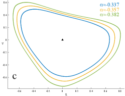
Phase portraits along (21) projected onto the plane (22) are shown in a series of six panels in Fig. 11; each corresponds to an interval annotated in Fig. 10(right). Near , we observe a family of growing invariant circles that pass through windows of periodicity as decreases. Panels (c),(d), and (f) show chaotic attractors; these occur when the segment (21) passes through gray regions, so that , in Fig. 10(right). These attractors are born with a structure like the invariant circle, but also seem to fold around the neighboring, no-longer stable periodic orbits. In panel (f) the outer boundary of the chaotic attractor appears relatively smooth, and aligns with the former invariant circle, but its interior is much more complex. This attractor is also shown in 3D in Fig. 13(a).


VI.2 Chaotic Attractors
As we have known since Feigenbaum’s classic studies of 1D maps, chaos can arise from a self-similar accumulation of period-doubling bifurcations, i.e., a period-doubling cascade. Guckenheimer and Holmes (2002); Kuznetsov (2004) As we have seen for (1), cascades from the fixed point , Fig. 5, or from higher period orbits, at the ‘ends’ of the tongues, Fig. 7, do indeed lead to chaos.
When is small, the resulting chaotic attractors can resemble that of the 2D Hénon map. For case (SC), where , the heteroclinic orbits of Fig. 6 show the beginning of the development of a Hénon-like attractor through a period-doubling cascade of the fixed point. Continuing beyond the endpoint of the segment in Fig. 5 leads to the attractor is shown in Fig. 12(a), with a nearly 2D, horseshoe-like shape. Note that for , the map (1) is essentially 2D,¶¶¶ It becomes a semi-direct product of a linear map and a 2D quadratic map. Hampton and Meiss (2022) and for , its dynamics correspond to the classic Hénon map. Hénon (1976) Even when , these parameters are at the very edge of the chaotic region after the period-doubling cascade of the fixed point, close to an arm of the period- shrimp in Fig. 5. The attractor for this case is shown in Fig. 12(b).


In Ref. [Gonchenko et al., 2021b], parameters were found so that a 3D quadratic map conjugate to (1) has a a discrete Lorenz-like attractor. The corresponding parameters for (1) are . This case lies within the chaotic region below the NS bifurcation of the period-two orbit shown in Fig. 4(b). The resulting Lorenz-like attractor (with a lacuna) is shown in Fig. 12(c). We refer to the works of Gonchenko et al. Gonchenko and Gonchenko (2016); Gonchenko et al. (2021b) for more discussion of such attractors.
In §VI.1, we saw the development of chaotic attractors as decreased along the segment (21), recall Fig. 11(c,d,f). A three-dimensional plot of panel (f) is shown in Fig. 13(a) to better illustrate that it appears to lie near a paraboloid that opens up in the positive direction along the line , which is near the local unstable manifold of the fixed point . To illustrate some of the variations in geometry that can occur, five additional cases, using parameters in the gray region of Fig. 4(b) for case (MC), are also pictured in Fig. 13. As before, each of these appears to lie near a paraboloid. The attractors in panels (a) and (b) have arms or tentacles, some of which appear to go towards the fixed point . By contrast, in panels (b) and (c), the attractors more closely resemble invariant circles with additional folds. Finally, in panels (e) and (f) the attractors have an internal flower-like structure that fills out an annular region on the paraboloid.


VII Conclusions
Previous research on quadratic 3D maps has focused on the volume-preserving caseLomelí and Meiss (1998); Dullin and Meiss (2009) or on the existence and development of chaotic attractors. Gonchenko et al. (2005); Gonchenko and Gonchenko (2016); Gonchenko et al. (2021b) Here, we have explored a broader range of parameters and studied periodic and aperiodic, regular and chaotic attractors.
The simplest bifurcations of a 3D map were discussed in §II using the trace and second trace of the Jacobian as primary parameters and fixing the Jacobian determinant. These results were applied to the fixed points of the map (1) in §III. We focused on two primary parameters: the more “structural” parameter , that controls the type of bifurcation and, what can be viewed as the “primary unfolding” parameter, . Note that in our previous work on anti-integrability, it was the limit that corresponded to a non-deterministic limit where the dynamics is conjugate to a shift on a set of symbols.Hampton and Meiss (2022)
For our numerical studies, we chose two cases for the Jacobian : a strongly contracting case (SC)—where the map is nearly 2D—and a moderately contracting case (MC).
We showed in §IV that all bounded orbits of the orientation preserving 3D Hénon map lie within a cube about origin as illustrated in Fig. 3. Most of the region of bounded orbits correspond to nonchaotic situations, which could be an attracting fixed point or orbits that arise from this point by doubling or Neimark-Sacker bifurcations. However this figure also shows protruding spikes from the region of stability, that may be related to attractors not born from the fixed point. We hope to study these further in the future.
To classify the behavior of bounded orbits, we computed resonant regions in parameter space in §V; these are analogous to the Arnold tongues of circle maps. The resulting partition of the bounded region, Fig. 4, shows periodic and aperiodic attractors. Using this, we are able to understand the development of attracting periodic orbits and visualize their codimension-one and -two bifurcations. Note that our computations used the attractor arising from a single initial condition. There will be cases with multiple attractors and cases for which the chosen orbit is unbounded even when there might be attractors elsewhere. But given the similarity between Fig. 3 and Fig. 4, the latter possibility is rare. We plan to investigate the more complex, outlying cases in future research.
Aperiodic attractors (defined to be attractors with period greater than ), were studied in §VI. We also followed the evolution of invariant circles along several curves in parameter space starting at points on the NS bifurcation curve where the rotation number was irrational. We did not attempt to follow a circle with fixed rotation number, though we expect such a curve exists in a two-dimensional parameter space and plan to do this in future research. Along the parameter curves that we did follow, the invariant circle has a varying rotation number. When this becomes rational, the circle undergoes a resonant bifurcation, generically breaking up into a pair of periodic orbits. As the curve leaves a resonant tongue, an invariant circle can reform. In some cases the destruction of the circle gave rise to chaotic attractors.
Some of the chaotic attractors we studied are well-known: the discrete Lorenz and Hénon attractors found in Refs. [Gonchenko et al., 2021b; Hénon, 1976; Hampton and Meiss, 2022]. More unusual are the chaotic attractors with a paraboloid structure that arise from the destruction of the invariant circles, recall Fig. 13. These are not classified in Ref. [Gonchenko and Gonchenko, 2016] and are not obviously related to the 3D generalized horseshoes studied by Ref. [Zhang, 2016]. We believe that further study of such cases could lead to a broader understanding of attractors that lie within higher-dimensional generalizations of the Smale horseshoe. We plan to analyze these further in future research.
Appendix A Parameter space conversion
Here, the conditions for codimension-one and -two bifurcations as seen in the last column of Table 1 in terms of the trace and second trace are converted to conditions on . We are interested in the fixed point of (1), given by (8), thus, and are given by (10), and . We assume that , as in (2).
Provided that there are no singularities, the codimension-one bifurcation curves are easily found using (9):
| (SN) | (24) | |||||
| (PD) | ||||||
| (NS) |
for , and given by, (12), (13), respectively. The NS bifurcation is restricted to the interval .
Again, provided there are no singularities, the codimension-two bifurcations are all points that satisfy (9), but also require an expression for . The SNf bifurcation occurs at . Using to solve for the fixed point, then gives
| (SNf) | ||||
where is dependent on .
A Neimark-Sacker bifurcation with rotation number occurs at . Solving for the fixed point then gives
| (R) | ||||
where, again, is dependent on .
Acknowledgements.
The authors acknowledge support from the National Science Foundation grant DMS-1812481.Data Availability Statement
The data that supports the findings of this study are available within the article.
References
- Hénon (1976) M. Hénon, “A two-dimensional mapping with a strange attractor,” Comm. Math. Phys. 50, 69–77 (1976), https://doi.org/10.1007/BF01608556.
- Guckenheimer and Holmes (2002) J. Guckenheimer and P. Holmes, Nonlinear Oscillations, Dynamical Systems, and Bifurcations of Vector Fields, Appl. Math. Sci., Vol. 42 (Springer-Verlag, New York, 2002) https://doi.org/10.1007/978-1-4612-1140-2.
- Kuznetsov (2004) Y. Kuznetsov, Elements of Bifurcation Theory, 3rd ed., Appl. Math. Sci., Vol. 112 (Springer-Verlag, New York, 2004) https://doi.org/10.1007/978-1-4757-3978-7.
- Gonchenko et al. (2005) S. Gonchenko, I. I. Ovsyannikov, C. Simó, and D. Turaev, “Three-dimensional hénon-like maps and wild lorenz-like attractors,” Int. J. of Bifurcation and Chaos 15, 3493–3508 (2005), https://doi.org/10.1142/S0218127405014180.
- Devaney and Nitecki (1979) R. Devaney and Z. Nitecki, “Shift automorphisms in the Hénon mapping,” Communications in Mathematical Physics 67, 137–146 (1979), http://projecteuclid.org/euclid.cmp/1103905161.
- Benedicks and Carleson (1991) M. Benedicks and L. Carleson, “The dynamics of the Hénon map,” Annals of Math. 133, 73–169 (1991), https://doi.org/10.2307/2944326.
- Sterling and Meiss (1998) D. Sterling and J. Meiss, “Computing periodic orbits using the anti-integrable limit,” Phys. Lett. A 241, 46–52 (1998), https://doi.org/10.1016/S0375-9601(98)00094-2.
- Lomelí and Meiss (1998) H. Lomelí and J. Meiss, “Quadratic volume-preserving maps,” Nonlinearity 11, 557–574 (1998), https://doi.org/10.1088/0951-7715/11/3/009.
- Elhadj and Sprott (2009) Z. Elhadj and J. Sprott, “Classification of three-dimensional quadratic diffeomorphisms with constant Jacobian,” Front. Phys. China 4, 111–121 (2009), https://doi.org/10.1007/s11467-009-0005-y.
- Lenz, Lomelí, and Meiss (1999) K. Lenz, H. Lomelí, and J. Meiss, “Quadratic volume preserving maps: An extension of a result of Moser,” Regul. Chaotic Dyn. 3, 122–130 (1999), https://doi.org/10.1070/RD1998v003n03ABEH000085.
- Dullin and Meiss (2008) H. Dullin and J. Meiss, “Nilpotent normal forms for a divergence-free vector fields and volume-preserving maps,” Physica D 237, 155–166 (2008), https://doi.org/10.1016/j.physd.2007.08.014.
- Dullin and Meiss (2009) H. Dullin and J. Meiss, “Quadratic volume-preserving maps: Invariant circles and bifurcations,” SIAM J. Appl. Dyn. Sys. 8, 76–128 (2009), https://doi.org/10.1137/080728160.
- Gonchenko, Meiss, and Ovsyannikov (2006) S. V. Gonchenko, J. Meiss, and I. Ovsyannikov, “Chaotic dynamics of three-dimensional Hénon maps that originate from a homoclinic bifurcation,” Regul. Chaotic Dyn. 11, 191–212 (2006), https://doi.org/10.1070/RD2006v011n02ABEH000345.
- Hampton and Meiss (2022) A. Hampton and J. Meiss, “Anti-integrability for three-dimensional quadratic maps,” SIAM J. Appl. Dyn. Sys. 21, 650–675 (2022), https://doi.org/10.1137/21M1433289.
- Turaev and Shilnikov (1998) D. Turaev and L. Shilnikov, “An example of a wild strange attractor,” Mat. Sb. 189, 137–160 (1998), https://doi.org/10.1070/SM1998v189n02ABEH000300.
- Gonchenko and Gonchenko (2016) A. S. Gonchenko and S. Gonchenko, “Variety of strange pseudohyperbolic attractors in three-dimensional generalized Hénon maps,” Physica D: Nonlinear Phenomena 337, 43–57 (2016), https://doi.org/10.1016/j.physd.2016.07.006.
- Gonchenko, Simo, and Vieiro (2013) S. Gonchenko, C. Simo, and A. Vieiro, “Richness of dynamics and global bifurcations in systems with a homoclinic figure-eight,” Nonlinearity 26, 621–678 (2013), https://doi.org/10.1088/0951-7715/26/3/621.
- Gonchenko and I. (2017) S. V. Gonchenko and O. I., “Homoclinic tangencies to resonant saddles and discrete Lorenz attractors,” Discrete and Continuous Dynamical Systems - S 10, 273–288 (2017), https://doi.org/10.3934/dcdss.2017013.
- Gonchenko et al. (2021a) A. S. Gonchenko, M. S. Gonchenko, A. D. Kozlov, and E. A. Samylina, “On scenarios of the onset of homoclinic attractors in three-dimensional non-orientable maps,” Chaos: An Interdisciplinary Journal of Nonlinear Science 31, 043122 (2021a), https://doi.org/10.1063/5.0039870.
- Zhao et al. (2017) M. Zhao, C. Li, J. Wang, and Z. Feng, “Bifurcation analysis of the three-dimensional Hénon map,” Discrete Contin. Dynamical Systems - S 10, 625–645 (2017), https://doi.org/10.3934/dcdss.2017031.
- Richter (2002) H. Richter, “The generalized Hénon maps: Examples for higher-dimensional chaos,” Int. J. Bif. Chaos 12, 1371–1384 (2002), https://doi.org/10.1142/S0218127402005121.
- Gonchenko et al. (2021b) S. Gonchenko, A. Gonchenko, A. Kazakov, and E. Samylina, “On discrete Lorenz-like attractors,” Chaos 31, 023117 (2021b), https://doi.org/10.1063/5.0037621.
- Gonchenko et al. (2014) A. Gonchenko, S. V. Gonchenko, A. Kazakov, and D. Turaev, “Simple scenarios of onset of chaos in three-dimensional maps,” Int. J. Bif. Chaos 24, 1440005 (2014), https://doi.org/10.1142/S0218127414400057.
- Gonchenko, Gonchenko, and Turaev (2021) A. Gonchenko, S. Gonchenko, and D. Turaev, “Doubling of invariant curves and chaos in three-dimensional diffeomorphisms,” Chaos 31, 113130 (2021), https://doi.org/10.1063/5.0068692.
- Zhang (2016) X. Zhang, “Chaotic polynomial maps,” Int. J. Bif. Chaos 26, 1650131 (2016), https://doi.org/10.1142/S0218127416501315.
- Kuznetsov and Meijer (2019) Y. Kuznetsov and H. Meijer, Numerical Bifurcation Analysis of Maps, Vol. 34 (Cambridge University Press, Cambridge, 2019) https://doi.org/10.1017/9781108585804.
- Gallas (1994) J. Gallas, “Dissecting shrimps: Results for some one-dimensional physical models,” Physica A: Statistical Mechanics and its Applications 202, 196–223 (1994), https://www.sciencedirect.com/science/article/pii/0378437194901740.
- MacKay and Tresser (1987) R. MacKay and C. Tresser, “Some flesh on the skeleton: The bifurcation structure of bimodal maps,” Physica D 27, 412–422 (1987), https://doi.org/10.1016/0167-2789(87)90040-6.
- Façanha, Oldeman, and Glass (2013) W. Façanha, B. Oldeman, and L. Glass, “Bifurcation structures in two-dimensional maps: The endoskeletons of shrimps,” Physics Letters A 377, 1264–1268 (2013), https://doi.org/10.1016/j.physleta.2013.03.025.