Visual Prompt Tuning in Null Space for Continual Learning

As can be seen in Figure 1, those outputs of LayerNorm and qkv-transformations corresponding to the image tokens remain unaffected by the updates to the prompts. Hence, the essence of attaining the consistency objective Eq. (10) can be turned into analyzing how to keep the output of self-attention in Eq. (3) unchanged as the prompts are updated, i.e., satisfying:

However, the nonlinear operation (i.e., $\mathrm{softmax}$) and the potential higher-order term ${\bf W}_{k}^{\top}{\bf Z}^{\top}{\bf Z}{\bf W}_{v}$ arising from ${\bf K}_{\bf Z}^{\top}{\bf V}_{\bf Z}$ in Eq. (3) complicate the direct resolution of this objective. Specifically, the non-injection property of the $\mathrm{softmax}$ function causes non-unique solutions. The multiplication between ${\bf K}_{{\bf Z}_{t+1}^{\top}}{\bf V}_{{\bf Z}_{t+1}}$ derives a quadratic term $\mathrm{LN}({\bf P}_{t}+\Delta{\bf P})^{\top}\mathrm{LN}({\bf P}_{t}+\Delta{\bf P})$, which result in difficult optimization for $\Delta{\bf P}$.

To address this issue, we propose two sufficient conditions consisting solely of linear operations. Specifically, we split the process of self-attention into two primary stages, i.e., the Affinity described by Eq. (4) and the Aggregation outlined in Eq. (6). We can achieve Eq. (11) by ensuring the consistency of each stage:

We first analyze the consistency objective of Affinity, i.e., Eq. (12), for ${\bf Z}_{t}$ and ${\bf Z}_{t+1}$:

where $\sqrt{D}$ is omitted for simplicity. Upon fulfilling Eq. (12), we can obtain ${\bf S}_{{\bf Z}_{t}}={\bf S}_{{\bf Z}_{t+1}}$, corresponding to the output of Eq. (5). Subsequently, we analyze the consistency objective of Aggregation in Eq. (13), yielding results for ${\bf Z}_{t}$ and ${\bf Z}_{t+1}$ as:

Based on Eq. (12$-$17), we are able to derive the following two equations, respectively:

Note that we expect to further deduce Eq. (18) and Eq. (19) to obtain equations among $\mathrm{LN}({\bf P}_{t})$, $\mathrm{LN}({\bf P}_{t}+\Delta{\bf P})$ and $\Delta{\bf P}$. However, due to the square root and quadratic terms in the expressions of the standard deviations $\boldsymbol{\sigma}_{{\bf P}_{t}}$ and $\boldsymbol{\sigma}_{{\bf P}_{t}+\Delta{\bf P}}$, it is difficult to express $\boldsymbol{\sigma}_{{\bf P}_{t}+\Delta{\bf P}}$ in terms of $\boldsymbol{\sigma}_{{\bf P}_{t}}$ and $\boldsymbol{\sigma}_{\Delta{\bf P}}$. Consequently, it is challenging to derive a straightforward equation that relates $\mathrm{LN}({\bf P}_{t})$ and $\mathrm{LN}({\bf P}_{t}+\Delta{\bf P})$ through $\Delta{\bf P}$.

To simplify the problem, we introduce an additional constraint on the distribution of prompts. Concretely, we require that the updated prompts ${\bf P}_{t}+\Delta{\bf P}$ retain the same distribution as ${\bf P}_{t}$, i.e., meeting the following assumption:

In this way, we can establish a straightforward mathematical relationship connecting $\mathrm{LN}({\bf P}_{t}+\Delta{\bf P})$, $\mathrm{LN}({\bf P}_{t})$ and $\Delta{\bf P}$:

Consequently, we can apply Eq. (21) to simplify Eq. (18) and (19) as:

It should be noted that in Eq. 22 and Eq. 23 , ${\bf W}_{k}$, ${\bf W}_{v}$ and $\boldsymbol{\alpha}$ are pre-trained parameters kept frozen throughout the continual learning process. ${\bf Q}_{{\bf X}_{t}}$ and ${\bf S}_{{\bf P}_{t}}$ are two matrices derived from the input ${\bf X}_{t}$. As our objective is to ensure that the above two equations remain valid for the variables ${\bf Q}_{{\bf X}_{t}}$ and ${\bf S}_{{\bf P}_{t}}$, it is sufficient to meet the following conditions, in which ${\bf W}_{v}$ can be ignored whereas ${\bf W}_{k}$ remains crucial:

Now we have obtained the simplified formulas expressed by $\Delta{\bf P}$ in Eq. (24) and (25).

To sum up, we convert the overall consistency equation Eq. (11) into two sufficient conditions Eq. (12) and (13) for Affinity and Aggregation, respectively. Consequently, we derive two corresponding consistency conditions Eq. (24) and (25) expressed by the prompt update $\Delta{\bf P}$, under the constraint of invariant prompt distribution formulated in Eq. (20). The deduced conditions can satisfy the consistency objective in Eq. (10), thereby achieving the goal of eliminating the interference of the new task on the old task for visual prompt tuning.

As ${\bf Q}_{{\bf X}_{t}}=\mathrm{LN}({\bf X}_{t}){\bf W}_{q}+\boldsymbol{b}_{q}$, Eq. (24) implies that if the (transposed) prompt update can be orthogonal to the normalized previous input image tokens ${\bf X}_{t}$ projected with a second-order transformation matrices ${\bf W}_{q}{\bf W}_{k}^{\top}$ of the pre-trained ViT, the consistency for Affinity can be guaranteed. When we ignore the normalization and the bias term in ${\bf Q}_{{\bf X}_{t}}$, Eq. (24) can be simplified as ${\bf X}_{t}{\bf W}_{q}{\bf W}_{k}^{\top}\Delta{\bf P}^{\top}=\mathbf{0}$. The simplified condition is still essentially different from the consistency condition of linear layers (i.e., Eq. (9)) and that deduced in [26] (i.e., ${\bf X}_{t}\Delta{\bf P}^{\top}=\mathbf{0}$). It indicates the interaction between the image tokens and prompts within ViT layers is fundamentally distinct, leading to a unique consistency condition related to the second-order transformation matrices ${\bf W}_{q}{\bf W}_{k}^{\top}$ of the pre-trained model. Moreover, Eq. (25) is also an essential condition served as one of the sufficient conditions for the consistency of the whole ViT layer. It implies that if the prompt update can be orthogonal to the activated attention map generated by the image queries (${\bf Q}_{\bf X}$) and prompt keys (${\bf K}_{\bf P}$), the consistency of Aggregation can be achieved.

To jointly optimize Eq. (24) and (25), we need to solve $\Delta{\bf P}$ that can meet both equations concurrently. Here, we employ a separate optimization approach to get an approximate solution efficiently. Initially, it ensures $\Delta{\bf P}^{\top}$ is orthogonal to the subspace spanned by ${\bf Q}_{{\bf X}_{t}}{\bf W}_{k}^{\top}$ to satisfy Eq. (24). Subsequently, it makes $\Delta{\bf P}$ orthogonal to the subspace spanned by ${\bf S}_{{\bf P}_{t}}$ to satisfy Eq. (25).

Specifically, we use ${\bf P}_{\mathcal{G}}$ to denote the candidate parameter update generated by the optimizer for the prompts. We aim to obtain a projection matrix $\mathcal{B}$ such that $\Delta{\bf P}=\mathcal{B}{\bf P}_{\mathcal{G}}$. Following the previously mentioned separate optimization strategy, we first ensure $\Delta{\bf P}^{\top}$ is orthogonal to ${\bf Q}_{{\bf X}_{t}}{\bf W}_{k}^{\top}$ by the projection matrix $\mathcal{B}_{1}$: $\Delta{\bf P}^{\top}=\mathcal{B}_{1}{\bf P}_{\mathcal{G}}^{\top}$. Then $\Delta{\bf P}$ is made orthogonal to ${\bf S}_{{\bf P}_{t}}$ by another projection matrix $\mathcal{B}_{2}$: $\Delta{\bf P}=\mathcal{B}_{2}{\bf P}_{\mathcal{G}}$. Therefore, the objective of the optimization turns into obtaining the two projection matrices $\mathcal{B}_{1}$ and $\mathcal{B}_{2}$ to satisfy Eq. (24) and (25). Inspired by the null-space projection method [36], the bases of $\mathcal{B}_{1}$ and $\mathcal{B}_{2}$ correspond to the null-space bases of ${\bf Q}_{{\bf X}_{t}}{\bf W}_{k}^{\top}$ and ${\bf S}_{{\bf P}_{t}}$, respectively. We use ${\bf U}_{1,0}\in\mathbb{R}^{D\times R_{1}}$ and ${\bf U}_{2,0}\times\mathbb{R}^{M\times R_{2}}$ to denote the bases of the null spaces for ${\bf Q}_{{\bf X}_{t}}{\bf W}_{k}^{\top}$ and ${\bf S}_{{\bf P}_{t}}$, where $R_{1}$ and $R_{2}$ indicate their nullities. ${\bf U}_{1,0}$ and ${\bf U}_{2,0}$ can be obtained from the right singular vectors associated with the zero singular values, through the process of singular value decomposition (SVD) applied by $\mathrm{SVD}(({\bf Q}_{{\bf X}_{t}}{\bf W}_{k}^{\top})^{\top}{\bf Q}_{{\bf X}_{t}}{\bf W}_{k}^{\top})$ and $\mathrm{SVD}({\bf S}_{{\bf P}_{t}}^{\top}{\bf S}_{{\bf P}_{t}})$, respectively. In this way, we get the projection matrices $\mathcal{B}_{1}={\bf U}_{1,0}{\bf U}_{1,0}^{\top}\in\mathbb{R}^{D\times D}$ and $\mathcal{B}_{2}={\bf U}_{2,0}{\bf U}_{2,0}^{\top}\in\mathbb{R}^{M\times M}$, which are the solutions enabling $\Delta{\bf P}$ to jointly satisfy Eq. (24) and (25):

For the constraint Eq. (20), we incorporate an additional loss function aimed at penalizing the drift of prompt distribution, hence realizing a relaxed version of this constraint:

In Eq. (27), $\boldsymbol{\mu}_{{\bf P}_{t}}$ and $\boldsymbol{\sigma}_{{\bf P}_{t}}$ represent the target prompt distribution obtained in task $\mathcal{T}_{t}$, while $\boldsymbol{\mu}_{{\bf P}_{t+1}}$ and $\boldsymbol{\sigma}_{{\bf P}_{t+1}}$ denote the distribution to be optimized in task $\mathcal{T}_{t+1}$.

To sum up, we use Eq. (26) to realize Eq. (24) and (25), and use Eq. (27) to meet Eq. (20), thereby achieving the consistency objective Eq. (10) for anti-forgetting. We provide a full algorithm of our approach in the appendix A .

We further extend the consistency conditions Eq. (24) and (25) to multi-head self-attention, a common feature in current transformer-based models. Suppose there are $H$ heads and $d=D/H$ represents the dimension of each token in a head. We use ${\bf Q}_{{\bf X}_{t}.h}\in\mathbb{R}^{N\times d}$, ${\bf W}_{k.h}\in\mathbb{R}^{D\times d}$ and ${\bf S}_{{\bf P}_{t}.h}\in\mathbb{R}^{N\times M}$ to denote the corresponding matrices in Eq. (24) and (25) for the $h$-th head, respectively. The objective is to ensure these conditions are met across all heads, i.e., ${\bf Q}_{{\bf X}_{t}.h}{\bf W}_{k.h}^{\top}\Delta{\bf P}^{\top}=\mathbf{0}$ and ${\bf S}_{{\bf P}_{t}.h}\Delta{\bf P}=\mathbf{0}$, $\forall h\in\{1,2,\cdots,H\}$. Let $\mathbf{\Omega}_{1,t}=[{\bf Q}_{{\bf X}_{t}.1}{\bf W}_{k.1}^{\top};\cdots;{\bf Q}_{{\bf X}_{t}.H}{\bf W}_{k.H}^{\top}]\in\mathbb{R}^{HN\times D}$ and $\mathbf{\Omega}_{2,t}=[{\bf S}_{{\bf P}_{t}.1};\cdots;{\bf S}_{{\bf P}_{t}.H}]\in\mathbb{R}^{HN\times M}$ represent the concatenated matrices from all the heads, respectively. Based on block matrix properties, those two sets of conditions can be formulated as $\mathbf{\Omega}_{1,t}\Delta{\bf P}^{\top}=\mathbf{0}$ and $\mathbf{\Omega}_{2,t}\Delta{\bf P}=\mathbf{0}$. To sum up, The main difference between single-head and multi-heads is that the parameter update should be orthogonal to the subspace spanned by the concatenation matrices from all heads for multi-heads self-attention. Therefore, for the multi-heads variant, only an additional step of concatenation of the matrices from all heads is required in our algorithm.

In our experiments, we mainly utilize the VPT [13] with a ViT-B/16 backbone [9] pre-trained on ImageNet-21k. Additionally, we validate the effectiveness on the CLIP [27] model, wherein the visual prompts are inserted into the image encoder. Our experiments are conducted across 4 class-incremental benchmarks: 10- and 20-split CIFAR-100, 10-split ImageNet-R and 10-split DomainNet. We report the mean values of the final average accuracy and final average forgetting over 3 runs with different random seeds. Given that the null spaces of ${\bf Q}_{{\bf X}_{t}}{\bf W}_{k}^{\top}$ and ${\bf S}_{{\bf P}_{t}}$ may not always exist in practice, we compute the approximate null spaces and determine the nullities $R_{1}$ and $R_{2}$ in an adaptive manner, rather than the way suggested in [36]. For more detailed information regarding the experimental setups, please refer to Appendix B.

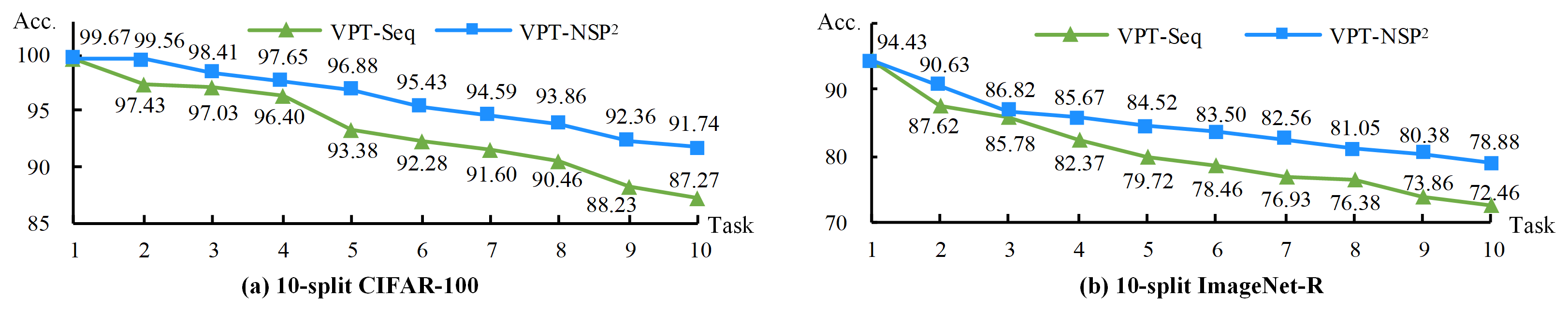
Validation of Effectiveness: The comparison between our approach and the sequential fine-tuning VPT and CLIP baselines is shown in Table 1 . For the VPT model, the proposed NSP² achieves 4.47%$\sim$10.26% improvements in accuracy on the 4 benchmarks. Meanwhile, it reduces the forgetting by 9.05%$\sim$17.11%. As to the CLIP model, the NSP² improves the accuracy by 6.48%$\sim$9.31%, and reduces the forgetting by 2.68%$\sim$17.27%. We calculate the accuracy across all previously encountered tasks after completing training on each task. The accuracy curves of VPT-Seq and VPT-NSP² on 10-split CIFAR-100 and 10-split ImageNet-R are displayed in Figure 2. They demonstrate our approach consistently outperforms the baseline throughout the sequential learning of tasks.

We conduct additional experiments with the VPT model, utilizing the weights pre-trained on different datasets as well as different paradigms, as shown in Figure 3 . The pre-training paradigms and datasets include: naive classification on ImageNet-1k [30], DINO [3] on ImageNet-1k, MIIL [29] on ImageNet21k-P and CLIP on LAION-2B [6] (we only use its image encoder). As can be seen from the figure, our approach not only significantly enhances accuracy but also markedly mitigates forgetting. These results further demonstrate the generalizability of the proposed approach.

Comparison with Existing Methods: We compare our method with existing methods in Table 2, where the competitors include many recent works. The proposed VPT-NSP² achieves state-of-the-art performance on the four benchmarks, with surpassing the second best approach by an average of 1.49% in accuracy. The forgetting of our approach is not the lowest, which is reasonable since our approach sacrifices some stability for a better trade-off between stability and plasticity. The outperforming accuracy can demonstrate the superiority of our method.

Ablation Study: The two consistency conditions Eq. (24) and (25), along with the constraint Eq. (20), constitute the main components of our approach. They correspond to $\mathcal{B}_{1}$, $\mathcal{B}_{2}$ in Eq. (26), and $\mathcal{L}_{\mathrm{LN}}$ in Eq. (27). We study their effects on the four benchmarks using VPT-NSP², with results presented in Table 3. We can see that the projection for Affinity ($\mathcal{B}_{1}$) plays a crucial role, which brings 3.31%$\sim$9.03% improvement in accuracy and 5.42%$\sim$14.76% decline in forgetting. Furthermore, the projection for Aggregation ($\mathcal{B}_{2}$) and the loss $\mathcal{L}_{\mathrm{LN}}$ for invariant prompt distribution are indispensable as well for minimizing forgetting. Optimal accuracy is achieved when all three conditions are applied.

Model Analysis: We analyze the evolution of training losses on the 10-split CIFAR-100 and 10-split ImageNet-R benchmarks, as shown in Figure 4 . Each point on the curve represents the training loss of the data in $\mathcal{T}_{1}$/$\mathcal{T}_{2}$ after the model has been trained on subsequent tasks. As can be seen, the losses of VPT-NSP² on previous tasks can be almost retained, confirming that our approach can effectively mitigate the interference of new tasks on old tasks.

Trade-off between Stability and Plasticity: We first adaptively determine the nullities $R_{1}$ and $R_{2}$ for $\mathcal{B}_{1}$ and $\mathcal{B}_{2}$ to achieve near-minimum forgetting. Based on this, we assign two weights $\eta_{1}$ and $\eta_{2}$ to the projection matrices to control the trade-off between stability and plasticity: $\Delta{\bf P}=\left[\eta_{2}\mathcal{B}_{2}+(1-\eta_{2}){\bf I}\right]{\bf P}_{\mathcal{G}}\left[\eta_{1}\mathcal{B}_{1}+(1-\eta_{1}){\bf I}\right]$, where ${\bf I}$ denotes the identity matrix. The effects of $\eta_{1}$ and $\eta_{2}$ which are set to a same value $\bar{\eta}$ is shown in Figure 5 . As the weight decreases, the accuracy increases first owing to better plasticity, and then decreases due to worse stability caused by the forgetting. It implies that a trade-off can be achieved by the two weights of projections.

Long-sequence Continual Learning We experiment on 5 benchmarks under the protocols of 50 tasks and 100 tasks to validate that our approach remains effective even within the context of long-sequence continual learning. The results are presented in Table 4. Despite lacking plasticity enhancement, VPT-NSP² can outperform existing state-of-the-art approaches and especially surpasses L2P by a large margin. This demonstrates that forgetting is still the predominant factor affecting performance in long sequence of tasks. With the plasticity enhancement, VPT-NSP² achieves significant increase in accuracy (by 1.1%$\sim$2.9%). This demonstrates that our plasticity enhancement is effective in learning new knowledge in long-sequence continual learning.

References

- [1] Lei Jimmy Ba, Jamie Ryan Kiros, and Geoffrey E. Hinton. Layer Normalization. CoRR, abs/1607.06450, 2016.
- [2] Benjamin Bowman, Alessandro Achille, Luca Zancato, Matthew Trager, Pramuditha Perera, Giovanni Paolini, and Stefano Soatto. À-la-carte Prompt Tuning (APT): Combining Distinct Data Via Composable Prompting. In IEEE/CVF Conference on Computer Vision and Pattern Recognition, pages 14984–14993, 2023.
- [3] Mathilde Caron, Hugo Touvron, Ishan Misra, Hervé Jégou, Julien Mairal, Piotr Bojanowski, and Armand Joulin. Emerging Properties in Self-Supervised Vision Transformers. In IEEE/CVF International Conference on Computer Vision, pages 9630–9640, 2021.
- [4] Arslan Chaudhry, Naeemullah Khan, Puneet K. Dokania, and Philip H. S. Torr. Continual Learning in Low-rank Orthogonal Subspaces. In Advances in Neural Information Processing Systems, 2020.
- [5] Kumar Chellapilla, Sidd Puri, and Patrice Simard. High performance convolutional neural networks for document processing. In Tenth international workshop on frontiers in handwriting recognition. Suvisoft, 2006.
- [6] Mehdi Cherti, Romain Beaumont, Ross Wightman, Mitchell Wortsman, Gabriel Ilharco, Cade Gordon, Christoph Schuhmann, Ludwig Schmidt, and Jenia Jitsev. Reproducible Scaling Laws for Contrastive Language-Image Learning. In IEEE/CVF Conference on Computer Vision and Pattern Recognition, pages 2818–2829, 2023.
- [7] Ekin D. Cubuk, Barret Zoph, Dandelion Mané, Vijay Vasudevan, and Quoc V. Le. AutoAugment: Learning Augmentation Strategies From Data. In IEEE/CVF International Conference on Computer Vision, pages 113–123, 2019.
- [8] Danruo Deng, Guangyong Chen, Jianye Hao, Qiong Wang, and Pheng-Ann Heng. Flattening Sharpness for Dynamic Gradient Projection Memory Benefits Continual Learning. In Advances in Neural Information Processing Systems, volume 34, pages 18710–18721, 2021.
- [9] Alexey Dosovitskiy, Lucas Beyer, Alexander Kolesnikov, Dirk Weissenborn, Xiaohua Zhai, Thomas Unterthiner, Mostafa Dehghani, Matthias Minderer, Georg Heigold, Sylvain Gelly, Jakob Uszkoreit, and Neil Houlsby. An Image is Worth 16x16 Words: Transformers for Image Recognition at Scale. In International Conference on Learning Representations, 2021.
- [10] Qiankun Gao, Chen Zhao, Yifan Sun, Teng Xi, Gang Zhang, Bernard Ghanem, and Jian Zhang. A Unified Continual Learning Framework with General Parameter-Efficient Tuning. In IEEE/CVF International Conference on Computer Vision, pages 11449–11459, 2023.
- [11] Zhanxin Gao, Jun Cen, and Xiaobin Chang. Consistent Prompting for Rehearsal-Free Continual Learning. CoRR, abs/2403.08568, 2024.
- [12] Wei-Cheng Huang, Chun-Fu Chen, and Hsiang Hsu. OVOR: OnePrompt with virtual outlier regularization for rehearsal-free class-incremental learning. In International Conference on Learning Representations, 2024.
- [13] Menglin Jia, Luming Tang, Bor-Chun Chen, Claire Cardie, Serge J. Belongie, Bharath Hariharan, and Ser-Nam Lim. Visual Prompt Tuning. In European Conference on Computer Vision, volume 13693, pages 709–727, 2022.
- [14] Dahuin Jung, Dongyoon Han, Jihwan Bang, and Hwanjun Song. Generating instance-level prompts for rehearsal-free continual learning. In IEEE/CVF International Conference on Computer Vision, pages 11813–11823, October 2023.
- [15] Muhammad Gul Zain Ali Khan, Muhammad Ferjad Naeem, Luc Van Gool, Didier Stricker, Federico Tombari, and Muhammad Zeshan Afzal. Introducing language guidance in prompt-based continual learning. In IEEE/CVF International Conference on Computer Vision, pages 11429–11439, October 2023.
- [16] Diederik P. Kingma and Jimmy Ba. Adam: A Method for Stochastic Optimization. In International Conference on Learning Representations, 2015.
- [17] Yajing Kong, Liu Liu, Zhen Wang, and Dacheng Tao. Balancing Stability and Plasticity Through Advanced Null Space in Continual Learning. In European Conference on Computer Vision, volume 13686, pages 219–236, 2022.
- [18] Muhammad Rifki Kurniawan, Xiang Song, Zhiheng Ma, Yuhang He, Yihong Gong, Yang Qi, and Xing Wei. Evolving Parameterized Prompt Memory for Continual Learning. In AAAI Conference on Artificial Intelligence, pages 13301–13309, 2024.
- [19] Zhuowei Li, Long Zhao, Zizhao Zhang, Han Zhang, Di Liu, Ting Liu, and Dimitris N. Metaxas. Steering Prototypes with Prompt-Tuning for Rehearsal-Free Continual Learning. In IEEE/CVF Winter Conference on Applications of Computer Vision, pages 2523–2533, 2024.
- [20] Yan-Shuo Liang and Wu-Jun Li. InfLoRA: Interference-free low-rank adaptation for continual learning. arXiv preprint arXiv:2404.00228, 2024.
- [21] Michael McCloskey and Neal J Cohen. Catastrophic interference in connectionist networks: The sequential learning problem. In Psychology of Learning and Motivation, volume 24, pages 109–165. Elsevier, 1989.
- [22] Mark D. McDonnell, Dong Gong, Amin Parvaneh, Ehsan Abbasnejad, and Anton van den Hengel. RanPAC: Random Projections and Pre-trained Models for Continual Learning. In Advances in Neural Information Processing Systems, 2023.
- [23] Thomas De Min, Massimiliano Mancini, Karteek Alahari, Xavier Alameda-Pineda, and Elisa Ricci. On the Effectiveness of LayerNorm Tuning for Continual Learning in Vision Transformers. In IEEE/CVF International Conference on Computer Vision Workshops, pages 3577–3586, 2023.
- [24] Adam Paszke, Sam Gross, Francisco Massa, Adam Lerer, James Bradbury, Gregory Chanan, Trevor Killeen, Zeming Lin, Natalia Gimelshein, Luca Antiga, Alban Desmaison, Andreas Köpf, Edward Z. Yang, Zachary DeVito, Martin Raison, Alykhan Tejani, Sasank Chilamkurthy, Benoit Steiner, Lu Fang, Junjie Bai, and Soumith Chintala. PyTorch: An Imperative Style, High-Performance Deep Learning Library. In Advances in Neural Information Processing Systems, pages 8024–8035, 2019.
- [25] Xingchao Peng, Qinxun Bai, Xide Xia, Zijun Huang, Kate Saenko, and Bo Wang. Moment Matching for Multi-Source Domain Adaptation. In IEEE/CVF International Conference on Computer Vision, pages 1406–1415, 2019.
- [26] Jingyang Qiao, Zhizhong Zhang, Xin Tan, Chengwei Chen, Yanyun Qu, Yong Peng, and Yuan Xie. Prompt Gradient Projection for Continual Learning. In International Conference on Learning Representations, 2024.
- [27] Alec Radford, Jong Wook Kim, Chris Hallacy, Aditya Ramesh, Gabriel Goh, Sandhini Agarwal, Girish Sastry, Amanda Askell, Pamela Mishkin, Jack Clark, Gretchen Krueger, and Ilya Sutskever. Learning Transferable Visual Models From Natural Language Supervision. In International Conference on Machine Learning, volume 139, pages 8748–8763, 2021.
- [28] Roger Ratcliff. Connectionist models of recognition memory: Constraints imposed by learning and forgetting functions. Psychological review, 97(2):285, 1990.
- [29] Tal Ridnik, Emanuel Ben Baruch, Asaf Noy, and Lihi Zelnik. ImageNet-21K Pretraining for the Masses. In NeurIPS Datasets and Benchmarks, 2021.
- [30] Olga Russakovsky, Jia Deng, Hao Su, Jonathan Krause, Sanjeev Satheesh, Sean Ma, Zhiheng Huang, Andrej Karpathy, Aditya Khosla, Michael S. Bernstein, Alexander C. Berg, and Li Fei-Fei. ImageNet Large Scale Visual Recognition Challenge. International Journal of Computer Vision, 115(3):211–252, 2015.
- [31] Gobinda Saha, Isha Garg, and Kaushik Roy. Gradient Projection Memory for Continual Learning. In International Conference on Learning Representations, 2021.
- [32] James Seale Smith, Leonid Karlinsky, Vyshnavi Gutta, Paola Cascante-Bonilla, Donghyun Kim, Assaf Arbelle, Rameswar Panda, Rogerio Feris, and Zsolt Kira. CODA-Prompt: COntinual Decomposed Attention-Based Prompting for Rehearsal-Free Continual Learning. In IEEE/CVF Conference on Computer Vision and Pattern Recognition, pages 11909–11919, June 2023.
- [33] Yu-Ming Tang, Yi-Xing Peng, and Wei-Shi Zheng. When Prompt-based Incremental Learning Does Not Meet Strong Pretraining. In IEEE/CVF International Conference on Computer Vision, pages 1706–1716, 2023.
- [34] Liyuan Wang, Jingyi Xie, Xingxing Zhang, Mingyi Huang, Hang Su, and Jun Zhu. Hierarchical Decomposition of Prompt-Based Continual Learning: Rethinking Obscured Sub-optimality. In Advances in Neural Information Processing Systems, 2023.
- [35] Runqi Wang, Xiaoyue Duan, Guoliang Kang, Jianzhuang Liu, Shaohui Lin, Songcen Xu, Jinhu Lv, and Baochang Zhang. AttriCLIP: A Non-Incremental Learner for Incremental Knowledge Learning. In IEEE/CVF Conference on Computer Vision and Pattern Recognition, pages 3654–3663, June 2023.
- [36] Shipeng Wang, Xiaorong Li, Jian Sun, and Zongben Xu. Training Networks in Null Space of Feature Covariance for Continual Learning. In IEEE/CVF Conference on Computer Vision and Pattern Recognition, pages 184–193, June 2021.
- [37] Yabin Wang, Zhiwu Huang, and Xiaopeng Hong. S-Prompts Learning with Pre-trained Transformers: An Occam’s Razor for Domain Incremental Learning. In Advances in Neural Information Processing Systems, 2022.
- [38] Yabin Wang, Zhiheng Ma, Zhiwu Huang, Yaowei Wang, Zhou Su, and Xiaopeng Hong. Isolation and Impartial Aggregation: A Paradigm of Incremental Learning without Interference. In AAAI Conference on Artificial Intelligence, pages 10209–10217, 2023.
- [39] Zifeng Wang, Zizhao Zhang, Sayna Ebrahimi, Ruoxi Sun, Han Zhang, Chen-Yu Lee, Xiaoqi Ren, Guolong Su, Vincent Perot, Jennifer G. Dy, and Tomas Pfister. DualPrompt: Complementary Prompting for Rehearsal-Free Continual Learning. In European Conference on Computer Vision, volume 13686, pages 631–648, 2022.
- [40] Zifeng Wang, Zizhao Zhang, Chen-Yu Lee, Han Zhang, Ruoxi Sun, Xiaoqi Ren, Guolong Su, Vincent Perot, Jennifer Dy, and Tomas Pfister. Learning to Prompt for Continual Learning. In IEEE/CVF Conference on Computer Vision and Pattern Recognition, pages 139–149, June 2022.
- [41] Ross Wightman. Pytorch image models. https://github.com/rwightman/pytorch-image-models, 2019.
- [42] Guanxiong Zeng, Yang Chen, Bo Cui, and Shan Yu. Continual Learning of Context-Dependent Processing in Neural Networks. Nature Machine Intelligence, 1(8):364–372, August 2019.
- [43] Gengwei Zhang, Liyuan Wang, Guoliang Kang, Ling Chen, and Yunchao Wei. SLCA: Slow Learner with Classifier Alignment for Continual Learning on a Pre-trained Model. In IEEE/CVF International Conference on Computer Vision, pages 19091–19101, October 2023.
- [44] Zhen Zhao, Zhizhong Zhang, Xin Tan, Jun Liu, Yanyun Qu, Yuan Xie, and Lizhuang Ma. Rethinking Gradient Projection Continual Learning: Stability/Plasticity Feature Space Decoupling. In IEEE/CVF Conference on Computer Vision and Pattern Recognition, pages 3718–3727, June 2023.
- [45] Da-Wei Zhou, Hai-Long Sun, Han-Jia Ye, and De-Chuan Zhan. Expandable Subspace Ensemble for Pre-Trained Model-Based Class-Incremental Learning. CoRR, abs/2403.12030, 2024.
Appendix: Visual Prompt Tuning in Null Space for Continual Learning
Appendix A Algorithm
An overview and algorithm of our approach are provided in Figure 6 and Algorithm 1 , respectively. We first initialize the overall uncentered covariance matrices [36] and , as well as the null-space projection matrices and . During training, the cross-entropy loss for classification and the loss of prompt distribution are jointly utilized for optimization. Subsequently, we get the candidate prompt updates computed by the optimizer. Then is projected by the null-space projection matrices and for updating the prompts. After the convergence, we obtain the matrices and to temporarily store and for the data of the current task. Then they are used to update the uncentered covariance matrices and by addition. Finally, we update the null-space projection matrices using the uncentered covariance matrices, which will be used in the next task.
Algorithm 2 shows the process of computing a null-space projection matrix. First, an input uncentered covariance matrix is decomposed by SVD, from which we can get the singular values and right singular vectors. Next, we determine the nullity (i.e., the dimension of null space) of according to the maximum second derivative, which is introduced in Section C . Then we select right singular vectors corresponding to the smallest singular values considered close to 0 as the bases of null space. Finally, we compute the normalized projection matrix, which provides an upper bound for the scale of the projected gradients and prevents excessive gradient magnitudes. In our implementation, the null-space projection matrix is added by an identity matrix with a weight (specifically for and for ). is a hyper-parameter for the trade-off between stability and plasticity, which is also introduced in Section C
Appendix B Experimental Setups and Implementation Details
Models: We validate our approach on the Vision Transformer (ViT) [9] and CLIP [27] models in the experiments, whose backbones are both ViT-Base/16 [9]. The ViT is pre-trained on ImageNet-21k, and we insert 4 prompts into each of the 12 layers for fine-tuning, which is referred to as "VPT" [13]. The classifiers are dependently trained in each task and the orthogonal projection is not applicable to them. All the classifiers from the available tasks are concatenated to make prediction during inference. For the CLIP model pre-trained on the WebImageText, we insert 4 prompts into each of the first 3 layers of the image encoder, while the text encoder is kept frozen. The logit scale that serves as a learnable scalar parameter to scale the cosine similarities between image features and text features is also set to trainable. We observed a serious cross-task confusion among the tasks in the CLIP model. Hence, we follow [43] to utilize the class-wise mean and covariance of previous features extracted before the embedding projection head (i.e., the last linear layer of the image encoder) to refine the projection head, after the prompt tuning stage in each task.
Benchmarks: We conduct experiments under the class-incremental learning protocol, where the classes in each task are disjoint, and task identity is unknown during inference. Four class-incremental benchmarks with three widely used datasets are adopted: 10- and 20-split CIFAR-100, 10-split ImageNet-R [39] and 10-split DomainNet [25, 38]. For the CIFAR-100 dataset, the total of 100 classes are randomly split into 10 or 20 tasks, which can evaluate the ability to handle different numbers of tasks. We follow [39] to randomly split the 200 classes in ImageNet-R into 10 tasks, which forms the 10-split ImageNet-R benchmark. For the 10-split DomainNet, we follow the same dataset protocol adopted in [38] and [11] to select the top 200 classes with the most images from the original DomainNet [25], and randomly split them into 10 tasks with 20 classes per task. 25% samples of the training data in each dataset are picked as a validation set for searching optimal hyper-parameters.
Metrics: Formally, the final average accuracy and final average forgetting are defined as:
where is the number of tasks, is the accuracy of the -th model on the -th task samples, and is the accuracy of the -th model on the -th task samples.
Higher accuracy means the model performs better, while lower forgetting means stronger stability (i.e., the ability to retain old knowledge). However, lower forgetting does not always generate higher accuracy since the accuracy is also affected by plasticity (i.e., the ability to learn new knowledge). The accuracy is the main metric we should focus on as it reflects the precision of classification in practice.
Implementations Details: For all the datasets and models, the images fed into the models are resized to pixels and augmented by AutoAugment [7] during training. For the VPT-based models, we use the Adam optimizer [16] with , and a weight decay of to train 100 epochs with an initial learning rate of 0.01 and a batch size of 256 on all benchmarks. The learning rate is scaled by a factor of 0.1 at the 50-th and 80-th epoch. Our training losses consist of the cross-entropy loss for classification and the loss in Eq. (27) whose coefficient is set to 1. Through cross validation on the validation set, we set the temperatures in the cross-entropy loss to 28, 25, 30 and 30 for the 10-split CIFAR100, 20-split CIFAR100, 10-split ImageNet-R and 10-split DomainNet benchmarks. There are two hyper-parameters and used for the trade-off between stability and plasticity in null-space projection as introduced in Section C , and we set both of them to be 0.97, 0.95, 0.94 and 0.95 for the four benchmarks by cross validation.
As to the CLIP-based models, the differences in training settings are as follows. We train them for 20 epochs with the batch size of 220 and the learning rate 0.001 which decays at the 10-th and 16-th epoch. The temperatures are all set to 1 since the logit scale is trainable. and are set to 0.98 which is a proper value for all the benchmarks. We refine the embedding projection head for 50 epochs using the SGD optimizer with a learning rate of 0.001, a momentum of 0.9 and a weight decay of .
Appendix C Trade-off between Stability and Plasticity
Given that the null space of covariance matrix does not always exist in practice, Wang et al. [36] suggest approximating it by selecting the bases whose associated singular values approach zero, where the singular values smaller than a specified multiple (denoted as in our paper) of the smallest one are selected. However, we experimentally find this strategy and the experience for selecting are not suitable for prompt tuning in ViTs to determine the nullities and for the uncentered covariance matrices and in Algorithm 1 , which will be introduced afterwards. To solve this problem, we propose an adaptive nullity strategy to determine the nullities in an adaptive manner. Utilizing the characteristic that the curve of descending singular values forms an "L" shape, we divide the curve into two parts by the point where the gradient changes fastest to cover most of the small singular values. It is realized by calculating the maximum second derivative of the points: