ViPErLEED package I: Calculation of curves and structural optimization
Abstract
Low-energy electron diffraction (LEED) is a widely used technique in surface-science laboratories. Yet, it is rarely used to its full potential. The quantitative information about the surface structure, contained in the modulation of the intensities of the diffracted beams as a function of incident electron energy, LEED , is underutilized. To acquire these data, only minor adjustments would be required in most experimental setups, but existing analysis software is cumbersome to use and often computationally inefficient. The ViPErLEED (Vienna package for Erlangen LEED) project lowers these barriers, introducing a combined solution for user-friendly data acquisition, extraction, and computational analysis. These parts are discussed in three separate publications. Here, the focus is on the computational part of ViPErLEED, which performs highly automated LEED- calculations and structural optimization. Minimal user input is required, and the functionality is significantly enhanced compared to existing solutions. Computation is performed by embedding the existing Erlangen tensor-LEED package (TensErLEED). ViPErLEED manages additional parallelization, monitors convergence, and processes all input and output. This makes LEED more accessible to new users while minimizing the potential for errors and the manual labor. Added functionalities include intelligent structure-dependent defaults for most calculation parameters, automatic detection of bulk and surface symmetries and their relationship, automated search procedures that preserve the symmetry and speed up convergence, adjustments to the TensErLEED code to handle larger systems than before, as well as parallelization and optimization. Modern file formats are used as input and output, and there is a direct interface to the Atomic Simulation Environment (ASE) package. The software is implemented primarily in Python (version ) and provided as an open-source package (GNU GPLv3 or any later version). A structure determination of the - surface is presented as an example for the application of the software.
I Introduction
I.1 History and motivation: The untapped potential of LEED
Low-energy electron diffraction (LEED) is a versatile, quick and easy-to-use characterization technique routinely used in many surface-science laboratories. Acquiring LEED images typically takes minutes, limited more by the time it takes to move a sample into position than the actual measurement. The resulting LEED pattern offers a reciprocal-space fingerprint of the surface unit cell, where each “spot” corresponds to a beam of diffracted electrons that fulfills the constructive-interference Bragg condition of the 2D periodicity of the surface. These data can indicate whether a given sample preparation yields the desired surface structure. However, this snapshot of the reciprocal lattice is only a fraction of the full information available from LEED. Spot-profile analysis (SPA)LEED [1, 2], as well as analysis of the background [3], can offer information about defects and surface order. LEED can yield accurate positions for the atoms in the unit cell. In LEED , the intensities of the scattered electron beams are measured as a function of electron energy, tuned via the accelerating voltage . Since these “ curves” can also be calculated theoretically, experimental LEED- data can be directly compared to a structural model of a surface. Comparison between calculations and experiment is performed through the so-called factor, which evaluates agreement across the entire beam set and breaks it down into a single value [4, 5]. Thus, with a relatively quick and simple laboratory-based experiment, one can confirm or reject hypothetical surface models, perform local optimizations of the atomic coordinates in such a model, or obtain a robust fingerprint to confirm the reproducibility of sample preparation [6, 7].

Crucially, the hardware for these experiments is already present in many surface-science laboratories, and only minor adjustments are required to upgrade most standard LEED setups to LEED- capability. The bigger hurdles are the analysis of the data and the calculation of the theoretical curves based on a given model. ViPErLEED, presented here, is a comprehensive package that combines a simple hardware add-on with software for acquiring and extracting the data, and for calculating and comparing to theoretical curves. Figure 1 shows the workflow with input and output.
The whole package consists of three parts, which are presented in three separate publications: The data acquisition (hardware), discussed in Part III [8]; the data extraction (spot tracking) and processing, discussed in Part II [9]; and the LEED- calculation and optimization, presented here. Specifically, this work discusses the software to calculate curves for a given reference structure and to optimize this structure based on the match with experimental data. While these three parts are optimized to be used together, they all employ standard file formats (such as comma-separated values — CSV) for input and output and can be used independently.
I.2 Basics of LEED
An extensive treatment of the theory of quantitative LEED, as well as the standard computational treatment, can be found in Refs. 10, 4, 11, 12, 13, 14, 7, 15, 16, 17, 6. These are only outlined briefly here to introduce important terms and concepts used in this work.
LEED is highly surface sensitive due to the low inelastic mean free path of electrons in solids (5–15 Å in the relevant energy range of up to 1000 eV [18]). Because of the strong electron–solid interaction, electrons typically experience multiple scattering events before leaving the surface [19]. Thus, calculations of LEED- spectra need to include paths with multiple scattering events. Crucially, small displacements (on the order of a few picometres) strongly affect the intensities of scattered beams. The high sensitivity to atomic positions gives LEED the potential for accurate determination of atomic coordinates. This, however, can only be achieved through a careful optimization process while comparing calculated and experimental curves.

Scattering of low-energy (–2000 eV) electrons with one atom in a solid is well approximated as occurring in a spherically symmetric potential (muffin-tin approximation) and conserving the angular momentum . Single scattering events of electrons with energy at a given site can then be described by partial-wave phase shifts . Electron–phonon scattering is included as an effective Debye–Waller factor, which depends on the vibration amplitudes of the atoms. Inelastic scattering is treated via an imaginary part of the inner potential, leading to an exponential decay with distance. The real part of the inner potential is defined by an approximate function, derived together with the scattering phase shifts with a boundary condition to the vacuum [25, 26]. With these few approximations, one can perform full-dynamic calculations of the multiple scattering of electrons, yielding theoretical curves that can be compared to experiment [10].
In a typical LEED calculation, the surface is split into “layers”, which should be separated along the surface normal by distances of at least Å. Each layer can consist of one or multiple atoms. Multiple scattering within each layer is then evaluated in angular-momentum space, resulting in layer-diffraction matrices. Propagation and scattering between the layers can be treated in a plane-wave representation [14, 10]. Figure 2 shows a typical layer definition for an example system of medium complexity: the - surface [24]. This system will be referred to several times below, and it is one of the examples given in the ViPErLEED documentation (see the Supplemental Material [27]). This layering scheme also allows for straightforward treatment of scattering far below the surface: One or two layers are defined as a bulk repeat unit (e.g., Layer 4 in Fig. 2) with a given bulk repeat vector. This bulk unit can then be stacked through repeated doubling until the norm of the reflection and transmission matrices of the bulk remains unchanged between successive steps [14].
I.3 The tensor-LEED approximation

The “full-dynamic” LEED calculations discussed so far are computationally demanding. The most expensive part is the inversion of matrices needed for intralayer scattering, which scales as (–3, depending on the algorithm) for matrices. Intralayer scattering matrices have for atoms in the layer and a maximum angular momentum [7]. As discussed in Section I.2, the high sensitivity to atomic coordinates on the picometre scale implies that basic comparisons of theoretical models to experimental data require local optimization of these coordinates, entailing numerous calculations. The number of optimization parameters also scales with system size, with a concomitant increase in the number of trial calculations [28].
The so-called tensor-LEED approximation makes these optimizations more efficient: A full-dynamic calculation is performed only for a reference structure; changes to the diffraction intensities through small modifications of the reference structure are treated by first-order perturbation theory [11, 12, 13]. This approach is ideal for structural optimization aimed at improving the agreement between theoretical and experimental curves, as the full-dynamic calculation only needs to be performed once. The optimization can then be performed using much cheaper evaluations of a set of perturbations, which scale linearly with the number of parameters under variation [12]. Importantly, the initial structural guess must be close to the target structure: The tensor-LEED approximation breaks down for displacements of more than Å [12], and significant errors are already introduced much sooner. This means that new reference calculations must be performed when changes to the original structure become too large. It is worth noting that the tensor-LEED approximation is not limited to purely geometrical perturbations of the reference structure. Changes of atomic vibration amplitudes [29] and statistical chemical substitutions [30] (including vacancies) can be treated with the same method and even concurrently [7, p. 135].
Several implementations exist for calculating LEED- curves, most of which are derived from the pioneering works of Pendry [16], Tong [31], and Van Hove [10]. Perhaps the most widely known is the Barbieri–Van Hove symmetrized automated LEED (SATLEED) package and its derivatives (MSATLEED, SATCLEED, ATLMLEED) [32, 33]. Alternatives include TensErLEED [14], described below, as well as DL_LEED [34], LEED90 [35], CAVLEED [36], CLEED [37] and LEEDFIT [38], though the latter four do not implement the tensor-LEED approximation, while DL_LEED has a partial tensor-LEED implementation [39]. The various packages encompass different capabilities, but none automates the structure-optimization process. Recently, the AQuaLEED package was published to simplify use of the SATLEED codes through a Python wrapper program [40, 41] in a similar, though much less broad, approach as the ViPErLEED package described here. A Python wrapper has also been recently developed for CLEED [42].
The theoretical foundation and code architecture of the TensErLEED package are described in detail in Ref. 14. Briefly, the package consists of three main modules, shown in Fig. 3(a), which perform different segments of the LEED- calculation. The “reference-calculation” module performs full-dynamic LEED- calculations, producing the complex amplitudes of the diffracted beams, , as implemented previously in the Van Hove–Tong code [10]. In addition, it also stores information necessary for the tensor-LEED approximation in separate output files, named “Tensors” in Ref. 14. The second TensErLEED segment is a “delta-amplitudes” calculation, which computes the changes for a small perturbation to the position, vibration amplitude, or site occupation (including mixing of chemical species as described by the average -matrix approximation [43]) of an atom . These are calculated for all atoms under variation and for each step in a given atom’s range of displacements. The third segment, the “search”, aims for the set of that, together with the reference amplitudes , minimizes the factor (i.e., the disagreement) between the calculated and experimental beams. Simply put, the full-dynamic reference calculation is a “precise” LEED calculation for a given reference structure, while the calculation and “search” compose the structural optimization using tensor LEED.
Altogether, the TensErLEED package [14] is a powerful and versatile tool for LEED- calculations, but it has shortcomings. Employing the package with its custom settings demands significant experience and poses a serious burden of entry for LEED- experimenters.
ViPErLEED drastically simplifies the user experience and expands the functionality and performance of existing solutions. The Python package controlling the computational aspects is named viperleed.calc. It manages the LEED- calculations — acting as a wrapper for the established TensErLEED modules — and contains higher-level logic and automation. By defining suitable defaults based on the theoretical structure and experimental data, viperleed.calc dramatically cuts down the required user input. Moreover, it provides additional functionality, such as optimization procedures not supported in the tensor-LEED formalism, automatic detection and preservation of surface and bulk symmetries during structural optimization, and acceleration of calculations through automated search procedures and parallelization.
viperleed.calc is designed with the vast scientific Python ecosystem in mind and leverages established numerical and scientific libraries such as NumPy [44], SciPy [45], Matplotlib [46], and Scikit-learn [47]. At the same time, it has an open application programming interface for future projects to exploit its novel features, such as the automated plane-group symmetry detection and structure symmetrization introduced in Section II.4.2.
II Program Description
As mentioned in Section I.3, ViPErLEED is based on the TensErLEED package [14] used to perform the core LEED- calculations. These include the “full-dynamic” reference calculations, the calculation of amplitude changes as a function of parameter variations, as well as the search for an optimal combination of these variations. Input and output processing, as well as most high-level logic, are handled in a Python module named viperleed.calc, described in more detail below. Direct user interaction with the TensErLEED scripts is not required at any point. Some aspects of TensErLEED are also updated to a version 2.0 that is being released with, but independent of, the viperleed.calc Python package. The updated TensErLEED version is more computationally efficient and supports calculations on larger systems. For completeness, these changes are also briefly discussed in Section II.7. Finally, a graphical user interface (GUI) provides LEED pattern previews and can be used to generate input for the spot-tracking program [9].
The viperleed.calc package is optimized for UNIX-based systems (Linux, MacOS, and Windows subsystem for Linux – WSL). Running natively on Windows is possible, but it involves some additional installation steps and configuration of the Fortran compilers. Installation instructions and details on setting up Fortran compilers can be found in the ViPErLEED documentation available online [48] or in the Supplemental Material [27].
II.1 ViPErLEED workflow
LEED- users wishing to work with existing solutions like TensErLEED, mostly based on the Van Hove–Tong codes [10], are faced with several challenges. The first hurdle regards the input files: Specific input formats are expected, and these may be difficult for new users to understand. Specifically, standardized structure files, often obtained as a result of density-functional theory (DFT) calculations, cannot be used as input directly. Instead, they have to be translated to “LEED formats” manually, which is tiresome and error prone. The standard output files are also problematic. To the best of the authors’ knowledge, none of the existing codes applying tensor-LEED calculations output the optimized structure in a standard crystal-structure format. As an example, TensErLEED optimization returns only a list of indices corresponding to the displacements of individual atoms that minimize the factor [14]. Translating these raw indices back to atomic coordinates of the best-fit structure is, again, cumbersome and a likely source of mistakes. When multiple optimization steps are required, all of these steps must be performed by hand repeatedly. Lastly, users are often required to manually compile the source code at runtime. This is for example the case for TensErLEED: many array dimensions depend on the input data and Fortran 77 does not allow dynamic memory allocation.
viperleed.calc addresses these issues. It accepts input in a standard format and automatically translates it into the custom format required by TensErLEED. Likewise, TensErLEED outputs are translated back to the same standard formats by keeping track of the inputs and variations. viperleed.calc also removes the need for manual compilation at runtime. For each TensErLEED segment, it performs the steps shown in Fig. 3(b): (i) Translate the user input into the format required by TensErLEED, (ii) compile the relevant TensErLEED code with appropriate array dimensions, (iii) execute the compiled code as a subprocess with adequate parallelization and with real-time monitoring if required, and (iv) process the TensErLEED output, producing user-readable output or input for the next TensErLEED segment. The compilation and execution of source code is a potential safety threat, as the source files may be modified with malicious intent. To ensure that only the expected TensErLEED code is executed, viperleed.calc contains hardcoded checksums for all expected Fortran files, and by default will only compile and run files conforming to these checksums.
Finally, ViPErLEED also includes a “bookkeeping” utility that keeps track of the performed calculations. It automatically updates a plain-text file (history.info) with information about the run segments, the resulting factors, and optional notes by the user. Additionally, it archives input and output files for every calculation into a history directory.
II.2 Main ViPErLEED input
The main input parameters defining viperleed.calc behavior are passed via the PARAMETERS input file. In the minimal case, this file defines which segments of TensErLEED should be executed and provides some information on how to interpret the structure files. However, the PARAMETERS file also allows in-depth control of TensErLEED calculation parameters and ViPErLEED defaults. More information on these parameters and the choice of defaults will be given in Section II.4. A comprehensive list of parameters and their default values is found in the ViPErLEED documentation [48].
Other than the general run parameters, the only input strictly required for calculating curves is the structural data, that is, an atomic model for the diffracting surface. The chosen standard is the POSCAR format used by the Vienna ab-initio simulation package (VASP) [49]. This choice is based on the assumption that many LEED- calculations start from a DFT-optimized structure; POSCAR files can easily be generated by standard structure viewers such as VESTA [50]. However, structural data can also be passed to ViPErLEED directly from the atomic simulation environment (ASE) package [51], which supports a variety of structural formats. Note that the surface is required to face the direction, with the first two unit-cell vectors and in the surface plane. Additionally, viperleed.calc assumes the bottommost layers (lowest coordinates) to be bulklike. This means that symmetric slabs commonly used in DFT are not allowed. However, a ViPErLEED-compatible slab can be obtained from a standard “DFT slab” by cutting below the “fixed” bulklike layers.
If structural optimization is to be performed, viperleed.calc requires two additional inputs: experimental curves (file EXPBEAMS.csv), and instructions on optimization parameters and ranges (file DISPLACEMENTS). For curves, ViPErLEED uses standard CSV formatting for all input and output. The DISPLACEMENTS file defines the range over which each structural parameter is varied during tensor-LEED optimization, and can contain instructions about the order in which the parameters are optimized. Structural parameters that can be varied are (i) atom positions, (ii) vibration amplitudes, and (iii) site occupation (including changes of statistical chemical composition through, e.g., vacancies, dopants, or alloy constituents). For convenience, the DISPLACEMENTS file supports a variety of shorthand forms to address groups of atoms by element, layer, specific site type, or atom number. The exact syntax for the DISPLACEMENTS file is described in the ViPErLEED documentation [48]. Plane-group symmetries of the surface are automatically preserved by viperleed.calc during displacements, such that symmetry-equivalent atoms in the input structure are kept symmetry equivalent during the optimization, unless the user explicitly reduces the symmetry by setting the desired plane group in the PARAMETERS file (see Section II.4.2).
Besides the mandatory input discussed above, users can optionally provide additional files. Otherwise, these are automatically generated by viperleed.calc:
-
•
First, an IVBEAMS file that specifies the curves to be calculated. This can be automatically generated to match available experimental data. When no experimental data is given, IVBEAMS must be supplied by the user.
-
•
Second, a starting guess for vibration amplitudes [52] and site occupations. This information can be included in the VIBROCC file. Otherwise, sites are assumed to be “chemically pure”. If vibration amplitudes are not specified, an initial guess can be generated based on the Debye temperature of the material and the experimental sample temperature — both specified in PARAMETERS (see the ViPErLEED documentation [48] for more details). In addition, a scaling factor may be defined for groups of atoms to reflect differences in the coordination environments. For example, undercoordinated atoms at the surface are expected to have a larger vibration amplitude. Since the vibration amplitudes themselves are parameters in the tensor-LEED optimization, this approximation is sufficient to obtain a reasonable starting point even when the Debye temperature is not known precisely.
-
•
Finally, energy-dependent phase shifts for electrons scattering on each type of atom in the structure. If not provided by the user (via a PHASESHIFTS file), these phase shifts will be generated automatically based on the input structure, using the EEASiSSS program [25], distributed with the ViPErLEED package with permission by the author.
II.3 Main ViPErLEED output
ViPErLEED output files use the same formats as the input files. This ensures that, if further optimization steps are required, output from previous ViPErLEED runs can be used directly as input for subsequent runs. The optimized structure is written to the files POSCAR_OUT and VIBROCC_OUT, and calculated curves are again written in CSV format. In addition, viperleed.calc generates PDF files with plots comparing the calculated beams to experimental data, annotated with factors for each beam. Some plots as output by viperleed.calc for the - example system are shown in Fig. 4. More examples can be found in the ViPErLEED documentation [48]. During structural optimization, a PDF file illustrating the search progress and state of convergence is generated in addition to the text-based log files (see Fig. S1 of the Supplemental Material [27]).
For diagnostic purposes, several supplementary files are written during each viperleed.calc run and stored in a directory called SUPP. These include the inputs and outputs of the TensErLEED programs, as well as modified POSCAR files generated during the structure analysis for troubleshooting.
II.4 Structure analysis and dynamic defaults
As discussed in Section II.2, one goal of ViPErLEED is to reduce the number of parameters required as user input. While some TensErLEED parameters can simply be set to a default value that is normally appropriate, others must be chosen in accordance with the structure in question. However, in most cases, it is still possible to define case-specific defaults through educated guesses.
To give an example, the scattering phase shifts depend on the angular momentum . At large , the phase shifts become small. Since the computing time strongly depends on the values (Section I.3), a cutoff must be defined. viperleed.calc automatically selects the cutoff such that phase-shift values at are smaller than a user-defined threshold (parameter PHASESHIFT_EPS). Similar considerations apply to many parameters that can be determined from the structural input. For most low-to-medium-complexity cases, viperleed.calc requires user input of less than ten parameters for a standard optimization. A full list of parameters, their defaults, and descriptions on how they are determined is given in the ViPErLEED documentation [48], and some example inputs are included in the Supplemental Material [27]. Here, the focus is on two non-trivial sets of parameters that viperleed.calc detects from the structural input: the repeat unit of the bulk, and plane-group symmetry.
II.4.1 Detecting and constructing the bulk
The shape of the curves is strongly affected by (multiple) scattering events deep within the bulk, especially at high energies, where the mean free path of the electrons is long. The number of layers to be considered is determined dynamically during the full-dynamic LEED calculations. Hence, it is not sensible to provide slabs of fixed thickness as input; rather, the structural input should include a construction rule defining how to add additional bulk layers as required during the calculations. As discussed in Section I.2, this is implemented in TensErLEED through a bulk-doubling scheme [14, 6]. Two ingredients are needed: the repeat unit of the bulk, and a bulk repeat vector that, when applied iteratively, reconstructs the bulk structure. Since typical structure formats (like the POSCAR file) do not contain this information, it is necessary to either determine it automatically, or to include it explicitly as a user input. Both options are supported in viperleed.calc.
Detecting bulk repeat.
The user can manually define how many layers at the bottom of the slab constitute a bulk repeat unit (parameter N_BULK_LAYERS), as well as the bulk repeat vector (parameter BULK_REPEAT, see Fig. 2). However, viperleed.calc can also detect these automatically. It can determine the bulk repeat vector if the repeat unit of the bulk is explicitly provided (via N_BULK_LAYERS). It can even identify both if the slab contains at least two layers that are sufficiently bulklike. In this case, users only need to specify the limit below which the slab is bulklike (parameter BULK_LIKE_BELOW). To find a repeat unit, the program iteratively tests downwards translations that shift atoms of the -th layer from the bottom to make them coincide with the position of the bottommost atom in the slab. Then, it compares the slabs before and after translation; if the atomic positions in the bulklike region are identical (within the tolerance given by parameter SYMMETRY_EPS), the translation vector is accepted as a bulk repeat vector. Note that even when the repeat unit of the bulk is detected automatically as discussed above, the N_BULK_LAYERS and BULK_REPEAT parameters are written to the PARAMETERS file explicitly. This causes BULK_LIKE_BELOW to be ignored in subsequent runs of viperleed.calc, ensuring that the repeat vector detected originally is preserved.
Detecting surface superstructures.
Another property that can be detected automatically in the initialization stage of the calculation is the relationship between the surface and bulk in-plane unit cells, that is, the periodicity of surface superstructures with respect to the bulk. Again, this relationship can be defined manually (parameter SUPERLATTICE, given either in Wood’s notation or as a transformation matrix). It can also be detected automatically by checking all candidate in-plane translations, then choosing the smallest possible bulk unit cell. It is worth noting that when dealing with non-trivial surface-to-bulk relationships there may be multiple choices for the bulk unit cell and its orientation, which impact the numbering of diffraction spots. In such scenarios, users should ensure proper labeling of experimental beams. For this purpose, viperleed.calc generates an experiment-symmetry.ini file during initialization, containing details about detected unit cells and symmetry. This file can be utilized as an input for the ViPErLEED GUI to generate a “pattern file”. When employed with the ViPErLEED spot tracker [9], this facilitates consistent beam labeling between experiment and calculations.
Diagnostic files for bulk detection.
viperleed.calc provides two diagnostic files to confirm the correct detection of the bulk: First, POSCAR_bulk, containing the bulk unit cell constructed from BULK_REPEAT and the two smallest unit vectors and in the surface plane; second, POSCAR_bulk_appended, which is the original POSCAR with additional bulk units added at the bottom using the BULK_REPEAT vector. This allows a quick visual check of whether the detected bulk cell is aligned correctly with the slab and reproduces the bulk in all directions.
II.4.2 Symmetry detection and structure symmetrization
The symmetry of crystal surfaces can be one of the 17 plane symmetry groups (also called “wallpaper groups”) defined by the unit cell and rotation axes, as well as mirror and glide planes of the structure (see Fig. 5). This symmetry may already be known from DFT calculations, from scanning-probe measurements, or from a qualitative comparison of the LEED beams. It is normally desirable to preserve such a symmetry during structural optimization. Symmetry reduces the dimensionality of the parameter space, drastically speeding up the structure search. In current implementations of LEED- calculations, the user is required to identify symmetry-equivalent atoms, and to ensure they are displaced in a symmetry-equivalent manner during optimization. While this is relatively straightforward for simple symmetry groups, it carries a high potential for user error, for example, when threefold rotation axes are involved. Figure 5 shows how the wallpaper groups constrain in-plane displacements for symmetry-equivalent atoms. viperleed.calc provides fully automatic detection of the plane symmetry group and by default preserves the symmetry during optimization.

Determining the minimal surface unit cell.
To enforce some conventions and highlight the symmetry, viperleed.calc applies several automatic modifications to the unit cell in the structural input and output. First, unit cells are reduced to a minimum-circumference form while preserving the area, as shown in Fig. 6(a). This ensures that no higher-symmetry representation of a given structure is missed. An example is oblique cells that are reducible to a rectangular form: enforcing this transformation allows to find potential mirror planes. Second, for reasons of convention and simplicity, rhombic and hexagonal cells are expected in obtuse form (angle between and greater than 90∘). Acute unit cells are automatically transformed into obtuse while preserving handedness [Fig. 6(b)]. Third, to avoid ambiguous beam labeling, the first unit-cell vector of the bulk should always be taken as the shorter one. For example, for a rectangular bulk unit cell, a supercell is closer to square than a cell. However, this third point is not enforced, and viperleed.calc will only output a warning if the vectors are swapped.
Detecting rotation axes, glide, and mirror planes.
Once the unit-cell shape is set, viperleed.calc searches for rotation axes, glide planes, and mirror planes. The algorithm for finding the symmetry is briefly described in the following. First, it considers all rotational symmetries possible for the given unit-cell type (e.g., three- and six-fold rotations are only checked for hexagonal cells), and detects the highest-order rotation axes. Since only 2D operations are of interest, it is most efficient to use the sublayer [53] with fewest atoms, as it yields the smallest set of candidate operations. Such candidates are then tested for the whole slab. If any rotation axes are found, the origin of the unit cell is shifted to the highest-order axis; if there are multiple highest-order rotation axes, the one closest to the original unit-cell origin is picked, as shown in Fig. 6(c). At this point, it is sufficient to check for mirror and glide planes going through the origin or through of the unit cell. As seen in Fig. 5, this procedure uniquely determines the plane symmetry group.

If no rotation axis is found, mirror and glide symmetries are detected in analogy to rotational symmetries. In the minimum-circumference form of the unit cell, only the unit-cell-vector directions and and the diagonals and (plus all 30∘-rotated directions , etc. for hexagonal cells) need to be considered to find all possible mirror/glide planes [54]. The unit-cell origin is again shifted (by the smallest possible distance) to coincide with a mirror plane, or with a glide plane if no mirror plane was found, as shown in Fig. 6(d). In cases where the orientation of the mirror/glide planes is ambiguous (groups pm, pg, cm and pmg), the symmetry can be fully specified by indicating the direction of the mirror or glide plane through the origin. For example, pm indicates pm symmetry with mirror planes parallel to the axis. The identified plane group symmetry is printed to the viperleed.calc log file and added as a comment in the POSCAR file.
Symmetrization.
Once the symmetry has been determined, viperleed.calc performs a symmetrization step to correct minor errors potentially introduced, for example, by not-fully-converged DFT relaxations. Positions of atoms that are equivalent within a given tolerance (parameter SYMMETRY_EPS) are averaged such that they are equivalent within floating-point precision. Atoms that should be locked to a rotation axis or mirror plane snap to that position, as shown in Fig. 6(e). This can be helpful since LEED- calculations are sensitive to position deviations in the picometre range.
The applied symmetry group can also be reduced manually, for example when the surface is suspected to possess a lower symmetry than the initial input structure. The SYMMETRY_FIX parameter allows to manually set any plane symmetry subgroup of the automatically detected group, including p1 if symmetry should be turned off entirely. In addition to the SYMMETRY_FIX parameter, which globally modifies the symmetry to be used, there is also a more local option to deactivate or reduce symmetry only for specific operations in the DISPLACEMENTS file with the SYM_DELTA tag. However, since this will result in breaking the symmetry in subsequent runs, users are discouraged from utilizing the SYM_DELTA tag except for highly specific cases. More details on both types of symmetry reductions are found in the ViPErLEED documentation [48].
Detecting beam equivalence and beam assignment.
Superstructures often exhibit different symmetry than the underlying bulk. Hence, single terraces of a sample may feature multiple “patches” of the same superstructure mirrored or rotated relative to one another, as induced by the plane group of the bulk. Additionally, different terrace orientations may be present when the bulk possesses screw or glide symmetry (some well-known cases are, e.g., Si(001) [55] or Fe3O4(001) [56]). This induces corresponding rotation or mirroring of the superstructures.
Since symmetry-induced domains normally have sizes larger than the typical coherence length of the electron beam, they contribute to the diffraction pattern incoherently. Such effect must be considered to correctly match calculated and experimental curves. viperleed.calc dramatically simplifies the user experience in this respect: instead of requiring the user to specify which calculated beams contribute to each experimental beam and should be averaged together, it detects beam equivalence automatically, assuming a statistical distribution of symmetry-induced domains. It also does not require the user to manually assign calculated to experimental beams: it does so automatically based on the beam labels [e.g., is the first-order diffraction spot in the direction of the first reciprocal unit-cell vector of the bulk, ]. The automatic beam averaging is enabled by viperleed.calc’s capability to detect symmetry (Section II.4.2). The same algorithm used for the whole slab is applied to the bulk, extending the search also to glide planes and screw axes with translation vectors parallel to the surface normal.
II.5 Automation and parallelization
A typical LEED- optimization with TensErLEED proceeds as follows: (i) execution of a full-dynamic calculation for the starting guess structure; (ii) optimization along a given displacement direction; (iii) further optimizations along other directions. [Steps (ii) and (iii) are distinct because the TensErLEED search module only supports 1D displacements for atom positions, such that multiple executions are required to fully optimize 3D atomic positions.] Steps (i) and (iii) are repeated until convergence. In TensErLEED, the user must perform all of these steps manually. This becomes especially cumbersome as one segment’s output must be manually translated into an input for the next segment. viperleed.calc simplifies the workflow. First, it handles the input/output processing internally. Second, it allows arbitrary queuing of segments with the RUN parameter. Finally, it allows to specify multiple sets of displacements in the DISPLACEMENTS file, such that they are automatically executed in the requested order. These optimizations can be looped until the factor converges, allowing for an autonomous search in a wide parameter space. The ViPErLEED documentation [48] gives more details on the RUN parameter and DISPLACEMENTS file. As described in Section S1 of the Supplemental Material [27], viperleed.calc also speeds up each optimization run in TensErLEED by monitoring the search progress and adjusting convergence parameters accordingly.
Besides automating the optimization workflow, viperleed.calc also enhances the parallelization of LEED- calculations. The parallelization offered by the native TensErLEED code is limited to the “search” module. viperleed.calc introduces additional parallelization at the Python level. Parallelization is applied to the full-dynamic calculation by assigning individual energies to separate processes. This is possible since each energy step can be calculated independently from the others. This approach enables further acceleration through a dynamic use of at each energy: At low energies, where phase shifts of large angular momenta are negligible, small values are used. Parallelization is also applied to the calculation. Here, the atoms under variation are independent and can be calculated in a parallel manner. Note that, since the single calculations are vastly more computationally expensive than the overhead, the parallelization offered by viperleed.calc comes close to the efficiency theoretically achievable with parallelization directly in the Fortran code.
II.6 Advanced optimization
II.6.1 Mixed-termination surfaces
Many systems can sustain coexisting surface reconstructions. In such cases, the intensities measured experimentally originate from an incoherent superposition of the diffracted beams from each termination. Some packages (like TensErLEED [14] and MSATLEED [33]) already implement optimization for this scenario.
viperleed.calc provides a simplified interface to the multi-domain optimization implemented in TensErLEED. A multi-domain calculation can be started either by supplying paths to the input structures or by providing pre-existing reference calculations (and corresponding Tensor files). In the latter case, viperleed.calc automatically performs a consistency check for compatibility of the input files. If the consistency check fails, viperleed.calc determines which parameters are shared between the different structures, harmonizes the input, and performs new, mutually compatible, full-dynamic calculations. Structural optimization is then performed using the tensor-LEED approximation including the fractional coverage of the domains as an additional parameter.
II.6.2 Full-dynamic optimization
viperleed.calc also provides an option for optimizing parameters that are inaccessible to the tensor-LEED approximation. Examples are the incidence angles (polar) and (azimuthal) of the primary electron beam, the imaginary part of the inner potential , and the lattice parameters of the input unit cell. For the latter, a scaling factor can be applied to one of the unit-cell vectors, to both in-plane unit-cell vectors at once, or to all three at once (i.e., scaling the volume of the unit cell).
Optimization of these parameters is enabled through repeated full-dynamic calculations. A “full-dynamic optimization” is set up using the OPTIMIZE parameter. It supports defining the parameter to optimize, the initial step size of variation, and convergence criteria. It is important to note that this kind of full-dynamic optimization is computationally significantly more expensive than tensor-LEED-based optimizations.
II.7 TensErLEED version 2.0
Although ViPErLEED is backwards compatible with the most recent version of TensErLEED at the time of writing (version 1.6), it was expedient during development to also make some improvements on the TensErLEED codebase. This resulted in a new version 2.0 of TensErLEED [57], which is released with ViPErLEED but can also be used independently. Changes include some minor bug fixes, increased precision of some computational variables, and improved computational performance, especially of the full-dynamic “reference” calculation. The speed-ups mainly come from replacing custom matrix-algebra routines by better-optimized BLAS and LAPACK versions [58], skipping redundant calculations, and refactoring certain routines for more efficient memory access.
The user interface (i.e., format of the input and output files) in TensErLEED 2.0 was modified to extend the size limits of systems that can be calculated. Previous TensErLEED versions severely limited the size of the unit cell, as well as related quantities such as the number of diffracted beams to calculate. The TensErLEED 2.0 input now allows larger values. Furthermore, some variables that were obsolete in the TensErLEED code but were still required in the input were removed, and others (e.g., imaginary part of the inner potential VPI and the filament work function WORKFN) were moved from hardcoded values in a runtime-created Fortran script (muftin.f) to standard input parameters.
Modifications to the TensErLEED code by the Solid-State Physics group in Erlangen and the ViPErLEED team are released together with ViPErLEED under the terms of the GNU General Public License version 3 (or any later version) [59].
II.8 Ongoing development
The ViPErLEED version 1.0 released with this work is a fully functional open-source package, licensed under the GNU General Public License version 3 or later [59]. Further development is in progress and will be published on the GitHub repository [60].
Already in version 1.0, ViPErLEED can start calculations based on structure input in the form of ASE Atoms objects [51]. This interface will be expanded to allow full control of all ViPErLEED features. This should, for the first time, allow easy high-throughput LEED- calculations for automatically generated surface structures. Many computational groups in the field are currently striving to solve complex surface structures without relying on human intuition [61, 62, 63, 64, 65, 66, 67]. As demonstrated in Ref. 68, the factor can be used as a cost function for guiding machine-learned structure prediction. The sensitive feedback provided by LEED may provide an attractive and new use of the technique for structure search in conjunction with total energies yielded by DFT calculations. A major benefit of using LEED for structure determination is its direct link to experimental data.
Another major change currently under development concerns a replacement for the TensErLEED optimization (“search”) algorithm. While ViPErLEED will continue to use the TensErLEED code for the full-dynamic calculations and calculations of amplitude changes , the TensErLEED algorithm for finding the combination of that minimizes the factor is somewhat dated. In the future, the current one-dimensional, grid-bound search may be replaced by a continuous search by calculating values on demand. This would allow direct application of, and free choice among established global optimization algorithms available from many optimized Python packages (e.g., SciPy [45], Scikit-Optimze [69], Keras [70], Ray [71], JAX [72]). Most of these modern evolutionary or (stochastic) gradient-based algorithms are likely to be much more effective at optimizing the structure than the original custom algorithm implemented in TensErLEED.
III Benchmark result: The termination of
The ViPErLEED documentation (see Supplemental Material [27]) guides the user through the application of ViPErLEED on a few example systems [among others, Ag(100), Ni(110), and Ir(100)-O]. This section outlines the main results obtained with ViPErLEED on a “medium-complexity” oxide surface: The termination of -oriented hematite (-Fe2O3) [20, 21, 22]. An introduction to the system and details on sample preparation are given in the Supplemental Material [27].
To ensure adequate sample conductivity of this wide-bandgap semiconducting material, LEED- data were acquired on a slightly Ti-doped (0.03 at.%) film (see Section S2 in the Supplemental Material [27] for details on the growth). The Ti-doped films expose atomically flat, single-crystalline surfaces; their and structures are identical to those of undoped crystals [23, 24]. The termination was prepared through repeated cycles of sputtering (10 min at 1 keV, mbar Ar, nA/mm2) and annealing (30 min at 550∘C, mbar O2, 20∘C/min ramp rate). Before each LEED measurement, the sample was heated for 10–20 min at ∘C to desorb H2O [73]. The cleanliness and quality of the surface was ensured by x-ray photoelectron spectroscopy and scanning tunneling microscopy.
LEED measurements were acquired at room temperature with an Omicron SpectaLEED (LaB6 cathode, three grids, one microchannel plate), and a DMK 33GX265 camera (The Imaging Source Europe GmbH, 80 ms exposure, 0 dB gain, 15-frames averaging, binning), using an electron energy range of 30–750 eV ( eV steps). The extracted data span a total energy range of keV after averaging symmetry-equivalent beams. Flat-field correction was performed by acquiring reference videos on the sample plate (see Part II [9] for more details). Intensities were normalized to the energy-dependent net beam current, , corrected for the energy-dependent current drawn by the LEED electronics, . To minimize artifacts from the LEED grids, the data were averaged from two sets of measurements acquired at sample–grid distances different by 2 mm (more details in Part II [9]). The data were taken during night to avoid magnetic-field fluctuations induced by streetcars traveling in front of the building. Static magnetic fields were compensated with the help of two coils mounted outside the vacuum chamber (see also Part III [8]). Since the sample has plane-group symmetry, the LEED intensities at perpendicular incidence have mirror symmetry in only one direction and no rotational symmetry. The crystal was rotated around the in-plane direction to ensure that the incident beam lies in the mirror plane of the LEED pattern, i.e., to achieve identical curves of the and spots. This ensures that the incidence plane is perpendicular to the surface. In turn, this allows to fix the azimuthal angle of incidence in the calculations, such that only the polar one requires fitting.

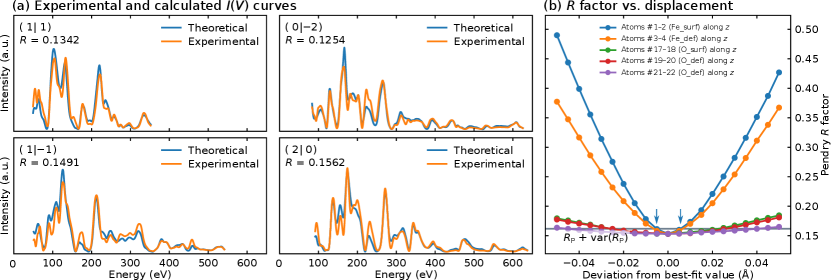
Figure 7 summarizes the outcome of a LEED- analysis performed with ViPErLEED on -. The Supplemental Material [27] includes the raw LEED data as well as final output files. It also describes in detail the steps leading to the optimization, as well as the parameters varied. Figure 7 shows two side views of the system, including values of atomic displacements predicted by the relaxed, lowest-energy DFT model (in parentheses), and by LEED- optimization. Figure 4(a) shows exemplary best-fit LEED- spectra to demonstrate the fit quality. All the experimental and calculated curves are plotted in Fig. S3 of the Supplemental Material [27]. The best-fit model of the structural analysis reproduces the measured LEED- spectra with an overall Pendry factor of . For educational purposes, LEED- optimization was started from a bulk-truncated slab [74] rather than the DFT-optimized model. The relaxations obtained by ViPErLEED and DFT are very close (within pm), and consistent within the uncertainty estimates that can be derived from LEED (see also Table S1 of the Supplemental Material [27]). The largest relaxations involve atoms of the topmost layer (cf. displacements marked in Fig. 7). At the surface, the Fe atoms relax downwards into the plane of the four surrounding O atoms, while O atoms from the first subsurface “sublayer” move closer to the surface. Effectively, this moves the Fe atoms of the topmost cation layer to coincide with the plane of their equatorial O atoms (distances from the plane decreased from pm to pm).
| Setup111Calculations were performed on the Vienna scientific cluster (VSC-4 [75]) on a node with two Intel® Xeon® Platinum 8174 processors, with a total of 96 logical cores, and 96 GB memory. The ifort compiler (version 2021.7.1) from the Intel® oneAPI® high-performance computing packages was used. All calculations used a maximum of two threads for LAPACK parallelization, by setting the oneAPI® math-kernel library MKL_NUM_THREADS environment variable. | 222Maximum angular momentum quantum number used for the expansion in spherical harmonics, as described in Section I.3. | N_CORES333Number of logical cores used for running calculations at different energies in parallel. See also Section II.5. | Execution time (min) |
|---|---|---|---|
| TensErLEED v1.6.0 | 12 | 1 | 89 |
| TensErLEED v2.0.0 | 12 | 1 | 69 |
| ViPErLEED444Using TensErLEED v2.0.0. | 6–12555Dynamically assigned by ViPErLEED with the default settings for the LMAX parameter. The same cutoff for phase shifts was employed in the calculation with dynamic as in the ones with fixed , but was evaluated independently at each energy, rather than using the determined at the highest beam energy for all calculations. | 1 | 63 |
| ViPErLEED4 | 6–125 | 48 |
Table 1 summarizes the duration of the full-dynamic calculations for the termination of reported in Fig. 7, as obtained with different setups. Through efficient use of parallelization, ViPErLEED produces results in less than 3 min, more than 30 times faster than the original TensErLEED configuration. This significant reduction of computation time not only enhances efficiency but also unlocks new opportunities for exploring larger, more complex, and previously inaccessible systems. More importantly, while harder to quantify, the time needed to set up this calculation with ViPErLEED is also on the order of minutes. In contrast, translating the structural and experimental data to TensErLEED input would be much more time intensive and error prone. For inexperienced users in particular, setting up the TensErLEED input for the first time can be daunting, given the numerous parameters with non-telling names that need definition. When the input contains mistakes, the Fortran modules crash, often without explanation. Instead, ViPErLEED requires only a handful of well-documented parameters. Moreover, it provides sensible feedback when executed, consisting of both fine-grained error messages, warnings based on a large number of “sanity checks”, as well as informative diagnostic files.
IV Conclusions
This work describes a new user-friendly and flexible open-source package for LEED- calculations and structural optimization, built on top and as an extension of the well-established TensErLEED package. This is part of the larger ViPErLEED project that also addresses data acquisition [8] and extraction [9]. Both the barrier of entry for new users and the potential for human error are significantly reduced by an expedient use of default parameters. The defaults are either static or automatically derived from properties of the experimental data and surface structure. Most significantly, surface symmetries are automatically detected and preserved during optimization. The program also automatically detects how calculated beams should be averaged and matched to an experimental beam set. All segments of LEED- calculations run under one combined user interface with standard input and output formats. Additional developments include simple optimization procedures for parameters inaccessible to the tensor-LEED approach, such as the incidence angle of the electron beam or the imaginary part of the inner potential. Computational performance of the TensErLEED package was improved both via top-level parallelization of the full-dynamic “reference” calculations and calculations of “delta amplitudes” , and through optimization directly in the TensErLEED code. This gain in speed and accuracy (in the sense of freedom from human errors) can be leveraged to perform LEED analysis of large systems that were previously impractical to tackle, as exemplified by a recent work on a surface-telluride phase with periodicity on Pt(111) [76].
Acknowledgements.
This research was funded in part by the Austrian Science Fund (FWF) under doi:10.55776/F81, Taming Complexity in Materials Modeling (TACO), and by the European Research Council (ERC) under the European Union’s Horizon 2020 research and innovation programme (grant agreement No. 883395, Advanced Research Grant ‘WatFun’). For the purpose of open access, the authors have applied a CC BY public copyright licence to any Author Accepted Manuscript version arising from this submission. Part of the LEED- calculations were performed on the Vienna Scientific Cluster (VSC). The authors extend their acknowledgments to all beta testers for reporting issues, and in particular to Jascha Bahlmann, Maximilian Buchta, Holger Diem, Julian Hochhaus, Jan Lachnitt, Matthias Meier, Simon Moser, Josef Mysliveček, Samuel Petrov, Karl-Michael Schindler, Alexander Schneider, and Martin Setvín for their valuable feedback. Furthermore, Matthias Blatnik, Jesús Carrete Montaña, Ralf Wanzenböck, Florian Buchner, Georg Madsen, Florian Libisch, and Christoph Schattauer are thanked for fruitful discussions. Finally, the authors are grateful for the permission to redistribute as part of ViPErLEED the EEASiSSS program for calculating phase shifts (John Rundgren) [25, 26, 38] and its dependencies (Eric Shirley) [77], as well as TensErLEED (Volker Blum and Klaus Heinz) [14]. Volker Blum, Klaus Heinz, and Eric Shirley are acknowledged for relicensing their contributions to TensErLEED and EEASiSSS under the terms of the GNU GPLv3 (or later).References
- Scheithauer et al. [1986] U. Scheithauer, G. Meyer, and M. Henzler, A new LEED instrument for quantitative spot profile analysis, Surf. Sci. 178, 441 (1986).
- Brand et al. [2024] C. Brand, A. Hucht, H. Mehdipour, G. Jnawali, J. D. Fortmann, M. Tajik, R. Hild, B. Sothmann, P. Kratzer, R. Schuetzhold, and M. Horn-von Hoegen, Critical behavior of the dimerized Si(001) surface: Continuous order-disorder phase transition in the two-dimensional Ising universality class, Phys. Rev. B 109, 134104 (2024).
- Starke et al. [1996] U. Starke, J. B. Pendry, and K. Heinz, Diffuse low-energy electron diffraction, Prog. Surf. Sci. 52, 53 (1996).
- Pendry [1980] J. B. Pendry, Reliability factors for LEED calculations, J. Phys. C 13, 937 (1980).
- Moore et al. [1982] W. T. Moore, D. C. Frost, and K. A. R. Mitchell, The Zanazzi-Jona and Pendry reliability indices compared in LEED crystallographic analyses for five surfaces, J. Phys. C 15, L5 (1982).
- Moritz and Van Hove [2022] W. Moritz and M. A. Van Hove, Surface Structure Determination by LEED and X-rays (Cambridge University Press, 2022).
- Heinz [2013] K. Heinz, Electron Based Methods: 3.2.1 Low-Energy Electron Diffraction (LEED), in Surface and Interface Science, edited by K. Wandelt (John Wiley & Sons, Ltd., 2013) Chap. 3.2, pp. 93–150.
- Dörr et al. [2024] F. Dörr, M. Schmid, L. Hammer, U. Diebold, and M. Riva, ViPErLEED package III: Data acquisition for low-energy electron diffraction, Phys. Rev. Research (2024).
- Schmid et al. [2024] M. Schmid, F. Kraushofer, A. M. Imre, T. Kißlinger, L. Hammer, U. Diebold, and M. Riva, ViPErLEED package II: Spot tracking, extraction and processing of curves, Phys. Rev. Research ADD DOI LINK (2024).
- Van Hove and Tong [1979] M. A. Van Hove and S. Y. Tong, Surface crystallography by LEED: theory, computation and structural results, Springer Series in Chemical Physics (Springer, Berlin, 1979).
- Rous et al. [1986] P. J. Rous, J. B. Pendry, D. K. Saldin, K. Heinz, K. Müller, and N. Bickel, Tensor LEED: A Technique for High-Speed Surface-Structure Determination, Phys. Rev. Lett. 57, 2951 (1986).
- Rous and Pendry [1989] P. J. Rous and J. B. Pendry, The theory of tensor LEED, Surf. Sci. 219, 355 (1989).
- Rous [1992] P. J. Rous, The tensor LEED approximation and surface crystallography by low-energy electron diffraction, Prog. Surf. Sci. 39, 3 (1992).
- Blum and Heinz [2001] V. Blum and K. Heinz, Fast LEED intensity calculations for surface crystallography using tensor LEED, Comput. Phys. Commun. 134, 392 (2001).
- Fauster et al. [2020] T. Fauster, L. Hammer, K. Heinz, and M. A. Schneider, Surface Physics: Fundamentals and methods, in Surface Physics (De Gruyter Oldenbourg, 2020).
- Pendry [1974] J. B. Pendry, Low Energy Electron Diffraction: The Theory and Its Application to Determination of Surface Structure, Techniques of Physics No. 2 (Academic Press, London, 1974).
- Van Hove et al. [1986] M. A. Van Hove, W. H. Weinberg, and C.-M. Chan, Low-Energy Electron Diffraction: Experiment, Theory and Surface Structure Determination, edited by G. Ertl and R. Gomer, Springer Series in Surface Sciences, Vol. 6 (Springer Verlag, Berlin, Heidelberg, 1986).
- Seah and Dench [1979] M. P. Seah and W. A. Dench, Quantitative electron spectroscopy of surfaces: A standard data base for electron inelastic mean free paths in solids, Surf. Interface Anal. 1, 2 (1979).
- foo [a] The multiple-scattering nature of electron–solid interaction is the main source of the high information density in LEED- data compared to, for example, surface-truncation rods in x-ray scattering.
- Henderson [2002] M. A. Henderson, Insights into the -to- phase transition of the -Fe2O surface using EELS, LEED and water TPD, Surf. Sci. 515, 253 (2002).
- Lad and Henrich [1988] R. J. Lad and V. E. Henrich, Structure of -Fe2O3 single-crystal surfaces following Ar+ ion-bombardment and annealing in O2, Surf. Sci. 193, 81 (1988).
- Tanwar et al. [2007] K. S. Tanwar, C. S. Lo, P. J. Eng, J. G. Catalano, D. A. Walko, G. E. Brown, Jr., G. A. Waychunas, A. M. Chaka, and T. P. Trainor, Surface diffraction study of the hydrated hematite surface, Surf. Sci. 601, 460 (2007).
- Franceschi et al. [2020] G. Franceschi, F. Kraushofer, M. Meier, G. S. Parkinson, M. Schmid, U. Diebold, and M. Riva, A model system for photocatalysis: Ti-doped single-crystalline films, Chem. Mater. 32, 3753 (2020).
- Kraushofer et al. [2018] F. Kraushofer, Z. Jakub, M. Bichler, J. Hulva, P. Drmota, M. Weinold, M. Schmid, M. Setvin, U. Diebold, P. Blaha, and G. S. Parkinson, Atomic-scale structure of the hematite “r-cut” surface, J. Phys. Chem. C 122, 1657 (2018).
- Rundgren [2003] J. Rundgren, Optimized surface-slab excited-state muffin-tin potential and surface core level shifts, Phys. Rev. B 68, 125405 (2003).
- Rundgren [2007] J. Rundgren, Elastic electron-atom scattering in amplitude-phase representation with application to electron diffraction and spectroscopy, Phys. Rev. B 76, 195441 (2007).
- [27] See Supplemental Material at URL for more details concerning: the sample; parameters used in the LEED- optimization and their best-fit value; DFT relaxation of the - structure; input files for the LEED- optimization, description of the optimization steps, and final outputs from both LEED and DFT; a copy of the ViPErLEED documentation; the source code for ViPErLEED version 1.0.0 and TensErLEED version 2.0.0; raw LEED- data for -. The Supplemental Material additionally cites Refs. 78, 79, 80, 81, 82, 83, 84, 85, 86, 87, 88, 89, 90, 91, 92, 93, 94, 95, 96, 97, 98, 99.
- Kottcke and Heinz [1997] M. Kottcke and K. Heinz, A new approach to automated structure optimization in LEED intensity analysis, Surf. Sci. 376, 352 (1997).
- Loffler et al. [1994] U. Loffler, R. Döll, K. Heinz, and J. B. Pendry, Investigation of surface atom vibrations by tensor LEED, Surf. Sci. 301, 346 (1994).
- Döll et al. [1993] R. Döll, M. Kottcke, and K. Heinz, Chemical substitution of surface atoms in structure determination by tensor low-energy electron diffraction, Phys. Rev. B 48, 1973 (1993).
- Tong [1975] S. Y. Tong, Theory of low-energy electron diffraction, Prog. Surf. Sci. 7, 1 (1975).
- Van Hove et al. [1993] M. A. Van Hove, W. Moritz, H. Over, P. J. Rous, A. Wander, A. Barbieri, N. Materer, U. Starke, and G. A. Somoraj, Automated-determination of complex surface-structures by LEED, Surf. Sci. Rep. 19, 191 (1993).
- [33] The Van Hove LEED packages are available for download on the internet, https://www.icts.hkbu.edu.hk/VanHove_files/leed/leedpack.html.
- Wander [2001] A. Wander, A new modular low energy electron diffraction package - DL_LEED, Comput. Phys. Commun. 137, 4 (2001).
- Blanco-Rey et al. [2004a] M. Blanco-Rey, P. de Andres, G. Held, and D. A. King, A FORTRAN-90 low-energy electron diffraction program (LEED90 v1.1), Comput. Phys. Commun. 161, 151 (2004a).
- Titterington and Kinniburgh [1980] D. J. Titterington and C. G. Kinniburgh, Calculation of LEED diffracted intensities, Comput. Phys. Commun. 20, 237 (1980).
- Held et al. [1996] G. Held, M. P. Bessent, S. Titmuss, and D. A. King, Realistic molecular distortions and strong substrate buckling induced by the chemisorption of benzene on Ni{111}, J. Chem. Phys. 105, 11305 (1996).
- Rundgren et al. [2021] J. Rundgren, B. E. Sernelius, and W. Moritz, Low-energy electron diffraction with signal electron carrier-wave wavenumber modulated by signal exchange-correlation interaction, J. Phys. Commun. 5, 105012 (2021).
- foo [b] Some integration modules for specific applications of LEED also exist in the literature [100, 101]. Structure-optimization algorithms dedicated to electron-diffraction data have also been developed [102, 103].
- Mayer et al. [2012] A. Mayer, H. Salopaasi, K. Pussi, and R. D. Diehl, A novel method for the extraction of intensity-energy spectra from low-energy electron diffraction patterns, Comput. Phys. Commun. 183, 1443 (2012).
- [41] https://github.com/andim/easyleed.
- [42] https://github.com/empa-scientific-it/cleedpy.
- Crampin and Rous [1991] S. Crampin and P. J. Rous, The validity of the average -matrix approximation for low-energy electron diffraction from random alloys, Surf. Sci. 244, L137 (1991).
- Harris et al. [2020] C. R. Harris, K. J. Millman, S. J. van der Walt, R. Gommers, P. Virtanen, D. Cournapeau, E. Wieser, J. Taylor, S. Berg, N. J. Smith, R. Kern, M. Picus, S. Hoyer, M. H. van Kerkwijk, M. Brett, A. Haldane, J. F. del Rio, M. Wiebe, P. Peterson, P. Gerard-Marchant, K. Sheppard, T. Reddy, W. Weckesser, H. Abbasi, C. Gohlke, and T. E. Oliphant, Array programming with NumPy, Nature 585, 357 (2020).
- Virtanen et al. [2020] P. Virtanen, R. Gommers, T. E. Oliphant, M. Haberland, T. Reddy, D. Cournapeau, E. Burovski, P. Peterson, W. Weckesser, J. Bright, S. J. van der Walt, M. Brett, J. Wilson, K. J. Millman, N. Mayorov, A. R. J. Nelson, E. Jones, R. Kern, E. Larson, C. J. Carey, I. Polat, Y. Feng, E. W. Moore, J. VanderPlas, D. Laxalde, J. Perktold, R. Cimrman, I. Henriksen, E. A. Quintero, C. R. Harris, A. M. Archibald, A. H. Ribeiro, F. Pedregosa, P. van Mulbregt, and SciPy 1.0 Contributors, SciPy 1.0: fundamental algorithms for scientific computing in Python, Nat. Methods 17, 261 (2020).
- Hunter [2007] J. D. Hunter, Matplotlib: A 2D graphics environment, Comput. Sci. Eng. 9, 90 (2007).
- Pedregosa et al. [2011] F. Pedregosa, G. Varoquaux, A. Gramfort, V. Michel, B. Thirion, O. Grisel, M. Blondel, P. Prettenhofer, R. Weiss, V. Dubourg, J. Vanderplas, A. Passos, D. Cournapeau, M. Brucher, M. Perrot, and É. Duchesnay, Scikit-learn: Machine learning in Python, J. Mach. Learn. Res. 12, 2825 (2011).
- vip [2024] The ViPErLEED documentation is available at https://www.viperleed.org and as part of the ViPErLEED GitHub repository [60] (2024).
- Kresse and Hafner [1993] G. Kresse and J. Hafner, Ab initio molecular dynamics for open-shell transition metals, Phys. Rev. B 48, 13115 (1993).
- Momma and Izumi [2011] K. Momma and F. Izumi, VESTA 3 for three-dimensional visualization of crystal, volumetric and morphology data, J. Appl. Crystallogr. 44, 1272 (2011).
- Hjorth Larsen et al. [2017] A. Hjorth Larsen, J. Jørgen Mortensen, J. Blomqvist, I. E. Castelli, R. Christensen, M. Dułak, J. Friis, M. N. Groves, B. Hammer, C. Hargus, E. D. Hermes, P. C. Jennings, P. Bjerre Jensen, J. Kermode, J. R. Kitchin, E. Leonhard Kolsbjerg, J. Kubal, K. Kaasbjerg, S. Lysgaard, J. Bergmann Maronsson, T. Maxson, T. Olsen, L. Pastewka, A. Peterson, C. Rostgaard, J. Schiøtz, O. Schütt, M. Strange, K. S. Thygesen, T. Vegge, L. Vilhelmsen, M. Walter, Z. Zeng, and K. W. Jacobsen, The atomic simulation environment – a Python library for working with atoms, J. Phys.: Condens. Matter 29, 273002 (2017).
- foo [c] The vibration amplitude as defined here (i.e., the square root of the value at temperature ) is based on the isotropic average of the squared 3D vibration displacements. These values may also include static disorder, such as small, random displacements due to defects or adsorbates.
- foo [d] A “sublayer” is defined as a set of chemically equivalent atoms with the same coordinate (within tolerance) to distinguish it from the notion of “layer” as used in TensErLEED: the latter is a composite object that may often be several ångströms thick. A “layer” is commonly composed of several “sublayers”.
- foo [e] Note that this approach implies that the correct symmetry may not be found if the POSCAR unit cell is not primitive in the surface plane. However, viperleed.calc will automatically recognize non-primitive unit cells, output a warning, and write a POSCAR_mincell file containing a slab with a primitive unit cell.
- Waltenburg and Yates [1995] H. N. Waltenburg and J. T. Yates, Surface-chemistry of silicon, Chem. Rev. 95, 1589 (1995).
- Bliem et al. [2014] R. Bliem, E. McDermott, P. Ferstl, M. Setvín, O. Gamba, J. Pavelec, M. A. Schneider, M. Schmid, U. Diebold, P. Blaha, L. Hammer, and G. S. Parkinson, Subsurface cation vacancy stabilization of the magnetite (001) surface, Science 346, 1215 (2014).
- [57] The source code for TensErLEED and EEASiSSS is hosted on GitHub. The TensErLEED code is currently maintained by the ViPErLEED team, https://github.com/viperleed/viperleed-tensorleed.
- Anderson et al. [1999] E. Anderson, Z. Bai, C. Bischof, S. Blackford, J. Demmel, J. Dongarra, J. Du Croz, A. Greenbaum, S. Hammarling, A. McKenney, and D. Sorensen, LAPACK Users’ Guide, 3rd ed. (Society for Industrial and Applied Mathematics, Philadelphia, PA, 1999).
- [59] https://www.gnu.org/licenses/gpl-3.0.en.html.
- [60] https://github.com/viperleed/viperleed.
- Noordhoek and Bartel [2024] K. Noordhoek and C. Bartel, Accelerating the prediction of inorganic surfaces with machine learning interatomic potentials, Nanoscale 16, 6365 (2024).
- Li et al. [2023] H. Li, Y. Jiao, K. Davey, and S.-Z. Qiao, Data-driven machine learning for understanding surface structures of heterogeneous catalysts, Angew. Chem., Int. Ed. 62, e202216383 (2023).
- Musa et al. [2022] E. Musa, F. Doherty, and B. R. Goldsmith, Accelerating the structure search of catalysts with machine learning, Curr. Opin. Chem. Eng. 35, 100771 (2022).
- Lee et al. [2023] Y. Lee, J. Timmermann, C. Panosetti, C. Scheurer, and K. Reuter, Staged training of machine-learning potentials from small to large surface unit cells: Efficient global structure determination of the RuO2(100)- reconstruction and (410) vicinal, J. Phys. Chem. C 127, 17599 (2023).
- Wanzenböck et al. [2022] R. Wanzenböck, M. Arrigoni, S. Bichelmaier, F. Buchner, J. Carrete, and G. K. H. Madsen, Neural-network-backed evolutionary search for SrTiO3(110) surface reconstructions, Digital Discovery 1, 703 (2022).
- Merte et al. [2022] L. R. Merte, M. K. Bisbo, I. Sokolović, M. Setvín, B. Hagman, M. Shipilin, M. Schmid, U. Diebold, E. Lundgren, and B. Hammer, Structure of an ultrathin oxide on Pt3Sn(111) solved by machine learning enhanced global optimization, Angew. Chem., Int. Ed. 61, e202204244 (2022).
- Hellström and Behler [2017] M. Hellström and J. Behler, Surface phase diagram prediction from a minimal number of DFT calculations: redox-active adsorbates on zinc oxide, Phys. Chem. Chem. Phys. 19, 28731 (2017).
- Primorac et al. [2016] E. Primorac, H. Kuhlenbeck, and H. J. Freund, LEED I/V determination of the structure of a MoO3 monolayer on Au(111): Testing the performance of the CMA-ES evolutionary strategy algorithm, differential evolution, a genetic algorithm and tensor LEED based structural optimization, Surf. Sci. 649, 90 (2016).
- Head et al. [2021] T. Head, M. Kumar, H. Nahrstaedt, G. Louppe, and I. Shcherbatyi, scikit-optimize/scikit-optimize (2021).
- Chollet et al. [2015] F. Chollet et al., Keras, https://keras.io (2015).
- Moritz et al. [2018] P. Moritz, R. Nishihara, S. Wang, A. Tumanov, R. Liaw, E. Liang, M. Elibol, Z. Yang, W. Paul, M. I. Jordan, and I. Stoica, Ray: A distributed framework for emerging AI applications, arXiv:1712.05889 (2018).
- Bradbury et al. [2018] J. Bradbury, R. Frostig, P. Hawkins, M. J. Johnson, C. Leary, D. Maclaurin, G. Necula, A. Paszke, J. VanderPlas, S. Wanderman-Milne, and Q. Zhang, JAX: composable transformations of Python+NumPy programs (2018).
- Jakub et al. [2019] Z. Jakub, F. Kraushofer, M. Bichler, J. Balajka, J. Hulva, J. Pavelec, I. Sokolovic, M. Müllner, M. Setvín, M. Schmid, U. Diebold, P. Blaha, and G. S. Parkinson, Partially dissociated water dimers at the water–hematite interface, ACS Energy Lett. 4, 390 (2019).
- Maslen et al. [1994] E. N. Maslen, V. A. Streltsov, N. R. Streltsova, and N. Ishizawa, Synchrotron x-ray study of the electron density in -Fe2O3, Acta Crystallogr. B 50, 435 (1994).
- [75] https://vsc.ac.at//systems/vsc-4/.
- Kißlinger et al. [2023] T. Kißlinger, A. Schewski, A. Raabgrund, H. Loh, L. Hammer, and M. A. Schneider, Surface telluride phases on Pt(111): Reconstructive formation of unusual adsorption sites and well-ordered domain walls, Phys. Rev. B 108, 205412 (2023).
- Shirley [1991] E. L. Shirley, Quasiparticle calculations in atoms and many-body core-valence partitioning, Ph.D. thesis, University of Illinois at Urbana-Champaign (1991).
- Kraushofer et al. [2021] F. Kraushofer, N. Resch, M. Eder, A. Rafsanjani-Abbasi, S. Tobisch, Z. Jakub, G. Franceschi, M. Riva, M. Meier, M. Schmid, U. Diebold, and G. S. Parkinson, Surface reduction state determines stabilization and incorporation of Rh on , Adv. Mater. Interfaces 8, 2001908 (2021).
- Kraushofer et al. [2022] F. Kraushofer, L. Haager, M. Eder, A. Rafsanjani-Abbasi, Z. Jakub, G. Franceschi, M. Riva, M. Meier, M. Schmid, U. Diebold, and G. S. Parkinson, Single Rh adatoms stabilized on by coadsorbed water, ACS Energy Lett. 7, 375 (2022).
- Gerhold et al. [2016] S. Gerhold, M. Riva, B. Yildiz, M. Schmid, and U. Diebold, Adjusting island density and morphology of the SrTiO3(110)- surface: Pulsed laser deposition combined with scanning tunneling microscopy, Surf. Sci. 651, 76 (2016).
- Blum et al. [2001] V. Blum, L. Hammer, W. Meier, K. Heinz, M. Schmid, E. Lundgren, and P. Varga, Segregation and ordering at Fe1-xAlx(100) surfaces – a model case for binary alloys, Surf. Sci. 474, 81 (2001).
- Ferstl et al. [2016] P. Ferstl, T. Schmitt, M. A. Schneider, L. Hammer, A. Michl, and S. Müller, Structure and ordering of oxygen on unreconstructed Ir(100), Phys. Rev. B 93, 235406 (2016).
- Johnson et al. [2000] K. Johnson, Q. Ge, S. Titmuss, and D. A. King, Unusual bridged site for adsorbed oxygen adatoms: Theory and experiment for Ir{100}-O, J. Chem. Phys. 112, 10460 (2000).
- Kißlinger et al. [2021] T. Kißlinger, M. A. Schneider, and L. Hammer, Submonolayer copper telluride phase on Cu(111): Ad-chain and trough formation, Phys. Rev. B 104, 155426 (2021).
- Sporn et al. [1998] M. Sporn, E. Platzgummer, S. Forsthuber, M. Schmid, W. Hofer, and P. Varga, The accuracy of quantitative LEED in determining chemical composition profiles of substitutionally disordered alloys: A case study, Surf. Sci. 416, 423 (1998).
- Kresse and Furthmüller [1996] G. Kresse and J. Furthmüller, Efficiency of ab-initio total energy calculations for metals and semiconductors using a plane-wave basis set, Comput. Mater. Sci. 6, 15 (1996).
- Blöchl [1994] P. E. Blöchl, Projector augmented-wave method, Phys. Rev. B 50, 17953 (1994).
- Kresse and Joubert [1999] G. Kresse and D. Joubert, From ultrasoft pseudopotentials to the projector augmented-wave method, Phys. Rev. B 59, 1758 (1999).
- Perdew et al. [1996] J. P. Perdew, K. Burke, and M. Ernzerhof, Generalized Gradient Approximation Made Simple, Phys. Rev. Lett. 77, 3865 (1996).
- Anisimov et al. [1991] V. I. Anisimov, J. Zaanen, and O. K. Andersen, Band theory and Mott insulators: Hubbard instead of Stoner , Phys. Rev. B 44, 943 (1991).
- Ovcharenko et al. [2016] R. Ovcharenko, E. Voloshina, and J. Sauer, Water adsorption and O-defect formation on Fe2O3(0001) surfaces, Phys. Chem. Chem. Phys. 18, 25560 (2016).
- Rollmann et al. [2004] G. Rollmann, A. Rohrbach, P. Entel, and J. Hafner, First-principles calculation of the structure and magnetic phases of hematite, Phys. Rev. B 69, 165107 (2004).
- George and Thompson [1967] P. K. George and E. D. Thompson, Debye temperature of nickel from 0 to 300 degrees K, J. Phys. Chem. Solids 28, 2539 (1967).
- Kim et al. [2001] J. G. Kim, K. H. Han, C. H. Lee, J. Y. Jeong, and K. H. Shin, Crystallographic and magnetic properties of nanostructured hematite synthesized by the sol-gel process, J. Korean Phys. Soc. 38, 798 (2001).
- De Grave et al. [1988] E. De Grave, L. H. Bowen, D. D. Amarasiriwardena, and R. E. Vandenberghe, Fe Mö-effect study of highly substituted aluminum hematites - determination of the magnetic hyperfine field distributions, J. Magn. Magn. Mater. 72, 129 (1988).
- Bødker et al. [2000] F. Bødker, M. F. Hansen, C. B. Koch, K. Lefmann, and S. Mørup, Magnetic properties of hematite nanoparticles, Phys. Rev. B 61, 6826 (2000).
- Morrish [1995] A. H. Morrish, Heat capacity and other thermodynamic quantities, in Canted Antiferromagnetism: Hematite (World Scientific Publishing Co. Pte. Ltd, Singapore, 1995) Chap. 5, pp. 76–80.
- Grønvold and Samuelsen [1975] F. Grønvold and E. J. Samuelsen, Heat-capacity and thermodynamic properties of -Fe2O3 in the region 300–1050 k. antiferromagnetic transition, J. Phys. Chem. Solids 36, 249 (1975).
- Catti et al. [1995] M. Catti, G. Valerio, and R. Dovesi, Theoretical study of electronic, magnetic, and structural properties of - (hematite), Phys. Rev. B 51, 7441 (1995).
- Blanco-Rey et al. [2004b] M. Blanco-Rey, P. de Andres, G. Held, and D. A. King, Molecular t-matrices for low-energy electron diffraction (TMOL v1.1), Comput. Phys. Commun. 161, 166 (2004b).
- de Andres and King [2001] P. L. de Andres and D. A. King, Anisotropic and anharmonic effects through the t-matrix for low-energy electron diffraction (TMAT v1.1), Comput. Phys. Commun. 138, 281 (2001).
- Blanco-Rey and de Andres [2006] M. Blanco-Rey and P. L. de Andres, Surface diffraction structure determination from combinatorial simultaneous optimization, Surf. Sci. 600, L91 (2006).
- Duncan et al. [2012] D. A. Duncan, J. I. J. Choi, and D. P. Woodruff, Global search algorithms in surface structure determination using photoelectron diffraction, Surf. Sci. 606, 278 (2012).