[table]style=plaintop \addauthorNumair [email protected] \addauthorMin H. [email protected] \addauthorJames [email protected] \addinstitution Brown University, USA \addinstitution KAIST, South Korea View-Consistent 4D Light Field Depth Estimation
View-consistent 4D Light Field
Depth Estimation
Abstract
We propose a method to compute depth maps for every sub-aperture image in a light field in a view consistent way. Previous light field depth estimation methods typically estimate a depth map only for the central sub-aperture view, and struggle with view consistent estimation. Our method precisely defines depth edges via EPIs, then we diffuse these edges spatially within the central view. These depth estimates are then propagated to all other views in an occlusion-aware way. Finally, disoccluded regions are completed by diffusion in EPI space. Our method runs efficiently with respect to both other classical and deep learning-based approaches, and achieves competitive quantitative metrics and qualitative performance on both synthetic and real-world light fields.
1 Introduction
Light fields allows high-quality depth estimation of fine detail by aggregating disparity information across many sub-aperture views. This typically results in a depth map for the central view of a light field only. However, in principle we can estimate depth for every pixel in the light field. Some applications require this ability, such as when editing a light field photograph when every output view will be seen on a light field display. Estimating depth reliably for disoccluded regions is difficult because it requires aggregating information from fewer samples. Few existing methods estimate depth for every light field pixel. These are typically computationally expensive [Wanner and Goldluecke(2012), Zhang et al.(2016)Zhang, Sheng, Li, Zhang, and Xiong] or not strictly occlusion aware. Jiang et al. [Jiang et al.(2019)Jiang, Shi, and Guillemot, Jiang et al.(2018)Jiang, Le Pendu, and Guillemot] presented the first practical view consistent method based on deep learning.
We present a counterpart first principles method with no learned priors, which produces comparable or better accuracy and view consistency than the current state of the art while being 2–4 faster. Our method is based around estimating accurate view-consistent disparity at edges, and then completing an occlusion-aware diffusion process to fill in missing regions.
Depth diffusion is a long-standing problem in which it is difficult to ensure both consistency and correctness in disoccluded regions. Our key contribution is an angular inpainting method that ensures depth consistency by design, while accounting for the visibility of points in disoccluded regions. In this way, we avoid the problem of trying to constrain or regularize view consistency after estimating depth spatially, and so can maintain efficiency.
Our code will be released as open source software at visual.cs.brown.edu/lightfielddepth.
2 Related Work
The regular structure of an Epipolar Plane Image (EPI) obviates the need for extensive angular regularization and, thus, many light field operations seek to exploit it. Khan et al.’s [Khan et al.(2019)Khan, Zhang, Kasser, Stone, Kim, and Tompkin] light field superpixel algorithm operates in EPI space to ensure a view consistent segmentation. The depth information implicit within an EPI is useful for disparity estimation algorithms. Zhang et al. [Zhang et al.(2016)Zhang, Sheng, Li, Zhang, and Xiong] propose an EPI spinning parallelogram operator for this purpose. This operator is similar in respects to the large Prewitt filters of Khan et al. [Khan et al.(2019)Khan, Zhang, Kasser, Stone, Kim, and Tompkin] but has a larger support, and provides more accurate estimates. A related method is presented by Tošić and Berkner [Tosic and Berkner(2014)] who create light field scale-depth spaces through convolution with a set of specially adapted kernels. Wang et al. [Wang et al.(2015)Wang, Efros, and Ramamoorthi, Wang et al.(2016)Wang, Efros, and Ramamoorthi] exploit the angular view presented by an EPI to address the problem of occlusion. Tao et al.’s [Tao et al.(2013)Tao, Hadap, Malik, and Ramamoorthi] work uses both correspondence and defocus in a higher-dimensional EPI space for depth estimation.
Beyond EPIs, Jeon et al.’s [Jeon et al.(2015)Jeon, Park, Choe, Park, Bok, Tai, and So Kweon] method exploits the relation between defocus and depth too. They shift light field images by small amounts to build a subpixel cost volume. Chuchwara et al. [Chuchvara et al.(2020)Chuchvara, Barsi, and Gotchev] present an efficient light-field depth estimation method based on superpixels and PatchMatch [Barnes et al.(2009)Barnes, Shechtman, Finkelstein, and Goldman] that works well for wide-baseline views. Efficient computation is also addressed by the work of Holynski and Kopf [Holynski and Kopf(2018)]. Their method estimates disparity maps for augmented reality applications in real-time by densifying a sparse set of point depths obtained using a SLAM algorithm. Chen et al. [Chen et al.(2018)Chen, Hou, Ni, and Chau] estimate occlusion boundaries with superpixels in the central view of a light field to regularize the depth estimation process.
With deep learning, methods have sought to bypass the large number of images in a light field by learning ‘priors’ that guide the depth estimation process. Huang et al.’s [Huang et al.(2018)Huang, Matzen, Kopf, Ahuja, and Huang] work can handle an arbitrary number of uncalibrated views. Alperovich et al. [Alperovich et al.(2018)Alperovich, Johannsen, and Goldluecke] showed that an encoder-decoder architecture can be used to perform light field operations like intrinsic decomposition and depth estimation for the central cross-hair of views. As one of the few depth estimation methods that operates on every pixel in a light field, Jiang et al. [Jiang et al.(2018)Jiang, Le Pendu, and Guillemot, Jiang et al.(2019)Jiang, Shi, and Guillemot] generate disparity maps for the entire light field and enforce view consistency. However, as their method uses low-rank inpainting to complete disoccluded regions, it fails to account for occluding surfaces in reprojected depth maps. Our method uses occlusion-aware edges to guide the inpainting process and so captures occluding surfaces in off-center views.
3 Occlusion-aware Depth Diffusion
A naive solution to estimate per-view disparity might be to attempt to compute a disparity map for each sub-aperture view separately. However, this is typically challenging for edge views and is highly inefficient, not only in terms of redundant computation but also due to the spatial domain constraints or regularization that must be added to ensure that depth maps are mutually consistent across views. Another simple approach might be to calculate a disparity map for a single view, and then reproject it into all other views. However, this approach fails to handle scene points that are not visible in the single source view. Such points cause holes in the case of disocclusions, or lead to inaccurate disparity estimates when the points lie on an occluding surface. While most methods try to deal with the former case through inpainting, for instance via diffusion, the latter scenario is more difficult to deal with as the occluding surface may have a depth label not seen in the original view. Thus, techniques like diffusion are insufficient on their own without additional guidance.
Our proposed method deals with this issue of depth consistency in subviews of light fields via an occlusion-aware diffusion process. We estimate sparse depth labels at edges that are explicitly defined across views, and then efficiently determine their visibility in each sub-aperture view. Given occlusion-aware edges which persist across views, these edge depth labels can be used as more reliable guides for filling any holes in reprojected views. Since the edge depth labels are not restricted to the source view, we capture any occluding surfaces not visible in the source view. This avoids the aforementioned problem of unseen depth labels. In addition, by performing our inpainting step in the angular rather than the spatial domain of the light field, we improve cross view consistency and occlusion awareness.
Edge Depth & Visibility Estimation
To begin, we estimate depth labels at all edges in the light field using the EPI edge detection algorithm proposed by Khan et al. [Khan et al.(2019)Khan, Zhang, Kasser, Stone, Kim, and Tompkin]. This filters each EPI with a set of large Prewitt filters, and then estimates a representation of each EPI edge as a parametric line. Lines in EPI space correspond to scene points, with the slope of the line being proportional to the depth of the point. Therefore, this line representation captures both position and disparity information of scene edges.
However, the parametric definition implies the line exists in all views, and, hence, the representation does not contain any visibility information for the point across light field views. We can address this by looking at local structure around the edge for point samples along the line: the point is visible if the local gradient matches the global line direction. We define a gradient-alignment-based visibility score for each sample, then threshold this score to decide which part of the line is actually visible in a given view [Khan et al.(2020)Khan, Kim, and Tompkin].
Given an EPI line , we sample it at locations to obtain a set of point samples on the EPI . Each sample corresponds to a projection of the original point in light field view , whose visibility can be determined as:
| (1) |
where denotes the characteristic function of a set beyond the visibility threshold, is the image gradient, is the direction perpendicular to the line , and .
The characteristic function was proposed by [Khan et al.(2020)Khan, Kim, and Tompkin] to generate a central view disparity map, and so only central view points were kept. By extending this idea to the entire light field, we retain all points along with their depth and visibility information, and use them to guide the disparity propagation into disoccluded and occluded regions. Since disparity directly at edges can often be ambiguous due to image resolution limits, the points are offset along the image gradient so that they lie on an actual surface. This is completed using the two-way propagation scheme of [Khan et al.(2020)Khan, Kim, and Tompkin], which also allows a disparity map for the central view to be generated using dense diffusion of the sparse point depths.
Cross-hair View Projection
The EPI line-fitting algorithm works on EPIs in the central cross-hair views—that is, the central row and column of light field images. While it is possible to run it on other rows and columns, this can become expensive, and the central set is usually sufficient to detect visible surfaces in the light field [Wanner and Goldluecke(2013)]. Hence, we project the estimated disparity map from the center view into all views along the cross-hair. Since gradients at depth edges in the estimated disparity map are not completely sharp, this leads to some edges being projected onto multiple pixels in the target view. We deal with this by sharpening the edges of the disparity map before projection, as shown in Shih et al. [Shih et al.(2020)Shih, Su, Kopf, and Huang], using a weighted median filter [Ma et al.(2013)Ma, He, Wei, Sun, and Wu] with parameters and . Omitting this step can cause inaccurate estimates around strong depth edges. The result is not very sensitive to parameters and since most parameter settings will target the error-prone strong edges.
Angular Inpainting
After depth reprojection, we must deal with the two problems highlighted in the overview: inpainting holes, and accounting for occluding surfaces in off-center sub-aperture views. We tackle this by using the edges from Section 3 to guide a dense diffusion process. Moreover, we ensure view consistency by performing diffusion in EPI space.
The EPI lines from the first stage constitute a set of cross-view edge features. is robust to occlusions in a single view as it exists in EPI space. As such, provides occlusion-aware sparse depth labels to guide dense diffusion in EPI space. Diffusion in EPI space has the added advantage of ensuring view consistency.
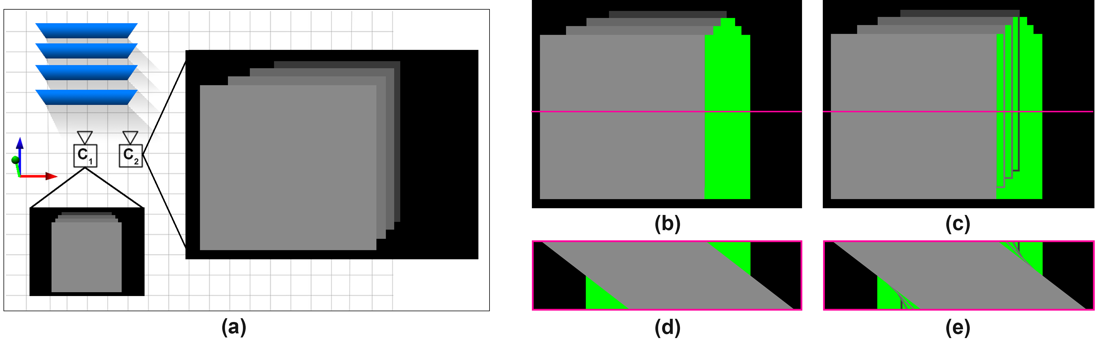
Let represent an angular slice of the disparity maps with values reprojected from the center view and with propagation guides (Figure 1). Then, we formulate diffusion as a constrained quadratic optimization problem:
| (2) |
where is the optimal depth labeling of the EPI, and is the set of four-connected neighboring pixels. The data and smoothness terms are defined as:
| (3) | ||||
| (4) |
We take the weight for the smoothness term from the EPI intensity image :
| (5) |
where . We define the weight for the data term as:
| (9) |
where is the edge-importance weight proposed by [Khan et al.(2020)Khan, Kim, and Tompkin], and and are the set of pixels coming from the reprojected center view disparity map and EPI line guides, respectively.
Equation (2) defines the optimal disparity map as one that minimizes divergence from the labeled data (Eq. (3)) while being as smooth as possible. Equation (4) measures smoothness as the similarity between disparities of neighboring pixels. We wish to relax the smoothness constraint for edges, so smoothness weight is chosen as the inverse of the image gradient (Eq. (5)). This allows pixels across edges to have a disparity difference without being penalized. The data weight (Eq. (9)) is determined empirically and works for all datasets.
Optimizing Equation (2) is a standard Poisson optimization problem. We solve this using the Locally Adaptive Hierarchical Basis Preconditioning Conjugate Gradient (LAHBPCG) solver [Szeliski(2006)] by posing the data and smoothness constraints in the gradient domain [Bhat et al.(2009)Bhat, Zitnick, Cohen, and Curless].
Non-cross-hair View Reprojection
We now have view-consistent disparity estimates for every pixel in the central cross-hair of light field views: , and . As noted, this set is usually large enough to cover every visible surface in the scene. Hence, all target views outside the cross-hair can be simply computed as the mean of the reprojection of the closest horizontal and vertical cross-hair view ( and , respectively).
4 Experiments
Baseline Methods
We compare our results to the state-of-the-art depth estimation methods of Jiang et al. [Jiang et al.(2018)Jiang, Le Pendu, and Guillemot] and Shi et al. [Shi et al.(2019)Shi, Jiang, and Guillemot]. Both methods use the deep-learning-based Flownet2.0 [Ilg et al.(2017)Ilg, Mayer, Saikia, Keuper, Dosovitskiy, and Brox] network to estimate optical flow between the four corner views of a light field, then use the result to warp a set of anchor views. In addition, Shi et al. further refine the edges of their depth maps using a second neural network trained on synthetic light fields. While Shi et al.’s method generates high-quality depth maps for each sub-aperture view, they do not have any explicit cross-view consistency constraint (unlike Jiang et al.).
Datasets
For our evaluation, we used both synthetic and real world light fields with a variety of disparity ranges. For the synthetic light fields, we used the HCI Light Field Benchmark Dataset [Honauer et al.(2016)Honauer, Johannsen, Kondermann, and Goldluecke]. This dataset consists of a set of four 9 9, 512 512 pixels light fields: Dino, Sideboard, Cotton, and Boxes. Each has a high-resolution ground-truth disparity map for the central view only. As such, we use this dataset to evaluate the accuracy of depth maps generated by our method and the baseline methods.
For real-world light field data, we use the EPFL MMSPG Light-Field Image Dataset [Rerabek and Ebrahimi(2016)] and the New Stanford Light Field Archive [sta(2008)]. The EPFL light fields are captured with a Lytro Illum and consist of views of pixels each. However, as the edge views tend to be noisy, we only use the central views in our experiments. We show results for the Bikes and Sphynx scenes. The light fields in the Stanford Archive are captured with a moving camera and have a larger baseline than the Lytro and synthetic scenes. Each scene consists of views with varying spatial resolution. We use all views from the Lego and Bunny scenes, scaled down to a spatial resolution of pixels.
Metrics
We evaluate both the accuracy and consistency of the depth maps. For accuracy, we use the mean-squared error (MSE) multiplied by a hundred, and the percentage of bad pixels. The latter metric represents the percentage of pixels with an error above a certain threshold. For our experiments we use the error thresholds 0.01, 0.03, and 0.07. The unavailability of ground truth depth maps for the EPFL and Stanford light fields prevents us from presenting accuracy metrics for the real world light fields.
To evaluate view consistency, we reproject the depth maps onto a reference view and compute the variance. Let represent the depth maps for the light field views warped onto a target view . The view consistency at pixel in view is given by:
| (10) |
and overall light field consistency is given as the mean over all pixels in the target view :
| (11) |
This formulation allows for the consistency to be evaluated quantitatively for both the synthetic and real world light fields.
We also compare computational running time. Our method is implemented in MATLAB except for the C++ Poisson solver. Both baseline methods use the authors’ implementations. The learning-based components of both baselines uses TensorFlow, with other components of Jiang et al. in MATLAB. All CPU code ran on an AMD Ryzen ThreadRipper 2950X 16-Core Processor, and GPU code ran on an NVIDIA GeForce RTX 2080Ti.
4.1 Evaluation
Accuracy
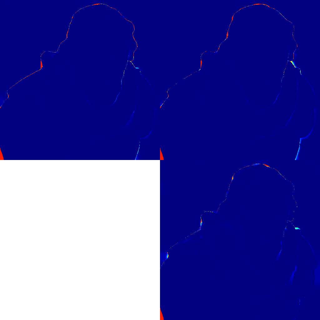
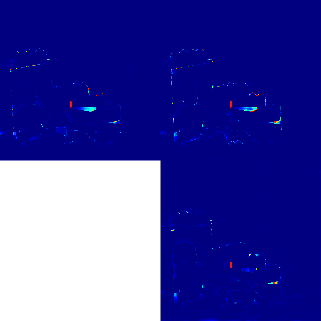
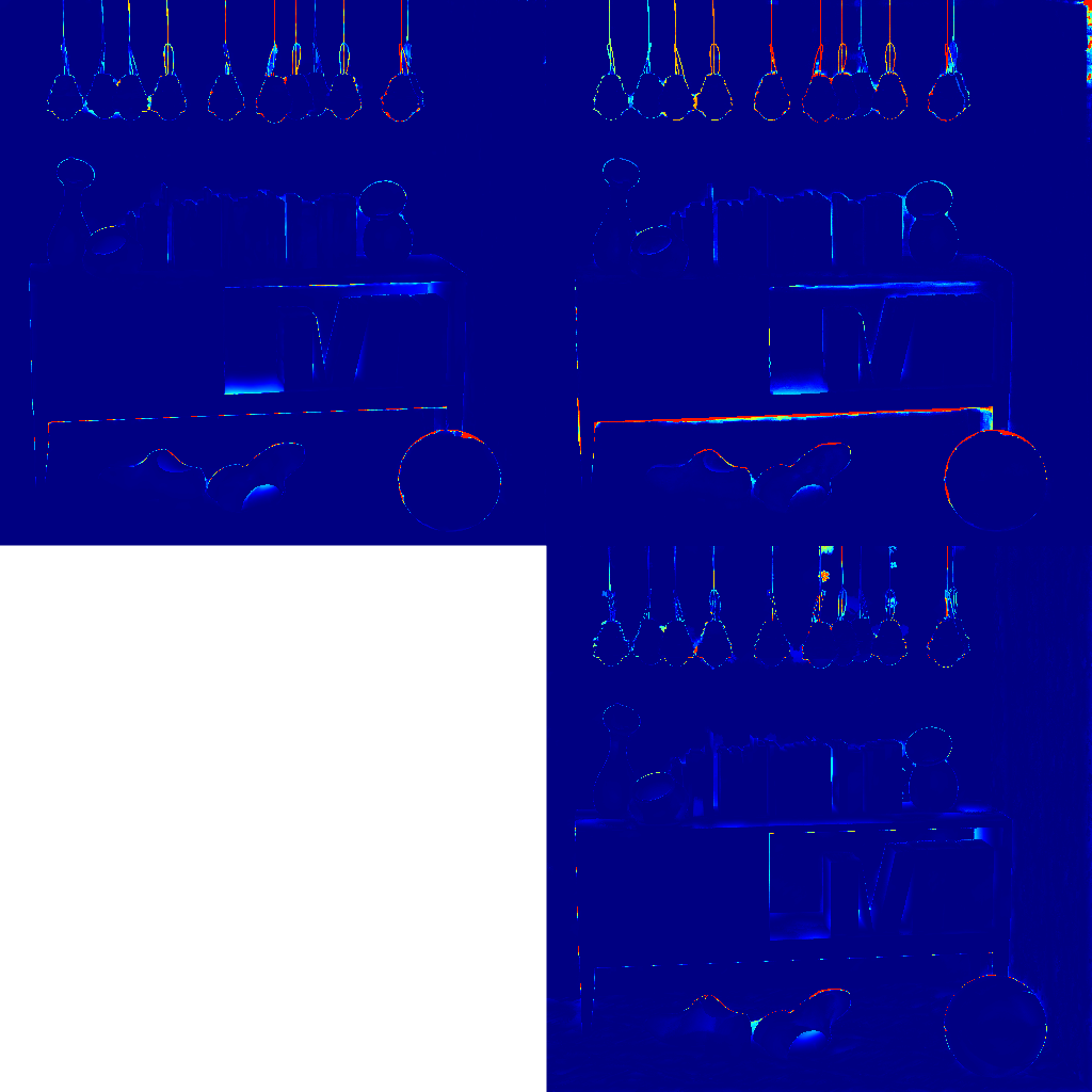
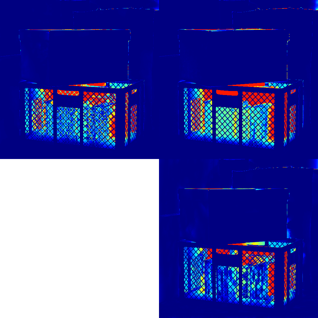
Table 1 presents quantitative results for the central view of all light fields in accuracy comparisons against ground truth depth. Our method is competitive or better on the MSE metric against the baseline methods, reducing error on average by 20% across the four light fields. However, our method produces more bad pixels than the baseline methods. For baseline techniques to have higher MSE but fewer bad pixels means that they must have larger outliers. This can be confirmed by looking at the error plots in Figure 5.
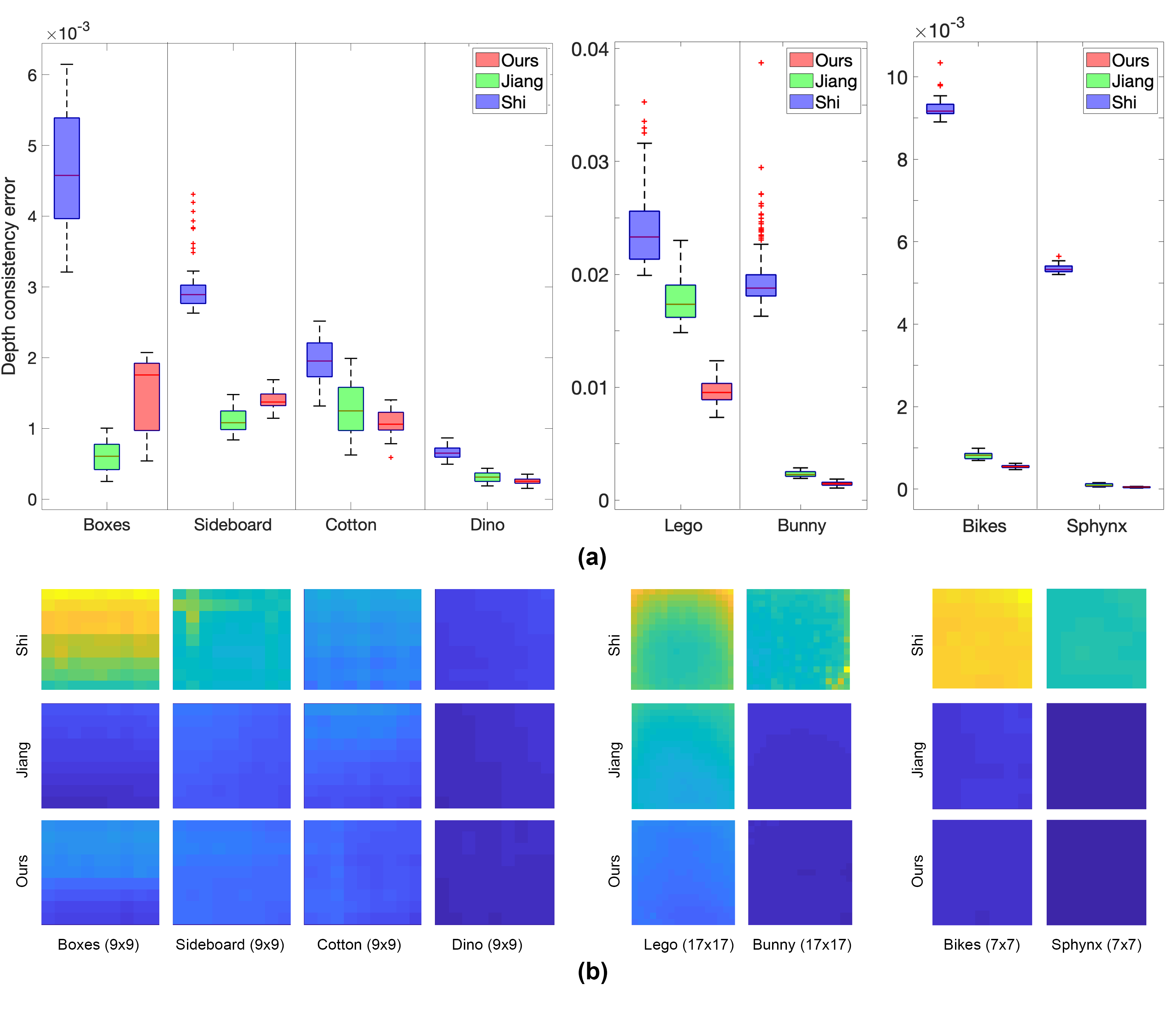
View Consistency
Figure 2 presents results for view consistency across all three datasets. The box plots at the top show that our method has competitive or better view consistency than the baseline methods. As expected, Shi et al.’s method without an explicit view consistency term has significantly larger consistency error. At the bottom of the figure, we visualize how this error is distributed spatially across the views in the light field. Both our method and Jiang et al.’s method produce relatively even distributions of error across views. In our supplemental video, we show view consistency error spatially for each light field view.
Computational Resources
Figure 3 presents a scatter plot of runtime versus view consistency across our three datasets. Our method produces comparable or better consistency at a faster runtime, being 2–4 faster than Jiang et al.’s methods per view for equivalent error.
[\FBwidth]

| Light Field | MSE * 100 | BP1(0.01) | BP2(0.03) | BP3(0.07) | ||||||||
|---|---|---|---|---|---|---|---|---|---|---|---|---|
| [Shi et al.(2019)Shi, Jiang, and Guillemot] | [Jiang et al.(2018)Jiang, Le Pendu, and Guillemot] | Ours | [Shi et al.(2019)Shi, Jiang, and Guillemot] | [Jiang et al.(2018)Jiang, Le Pendu, and Guillemot] | Ours | [Shi et al.(2019)Shi, Jiang, and Guillemot] | [Jiang et al.(2018)Jiang, Le Pendu, and Guillemot] | Ours | [Shi et al.(2019)Shi, Jiang, and Guillemot] | [Jiang et al.(2018)Jiang, Le Pendu, and Guillemot] | Ours | |
| Sideboard | 1.12 | 1.96 | 0.89 | 53.0 | 47.4 | 73.8 | 20.4 | 18.3 | 37.36 | 2.70 | 9.3 | 16.2 |
| Dino | 0.43 | 0.47 | 0.45 | 43.0 | 29.8 | 69.4 | 13.1 | 8.8 | 30.8 | 4.3 | 3.6 | 10.4 |
| Cotton | 0.88 | 0.97 | 0.68 | 38.8 | 25.4 | 56.2 | 9.6 | 6.3 | 18.0 | 2.8 | 2.0 | 4.9 |
| Boxes | 8.48 | 11.60 | 6.70 | 66.5 | 51.8 | 76.8 | 37.1 | 27.0 | 47.9 | 21.9 | 18.3 | 28.3 |
| Mean | 2.72 | 3.75 | 2.18 | 50.3 | 38.6 | 69.0 | 20.1 | 15.1 | 33.5 | 7.9 | 8.3 | 14.9 |
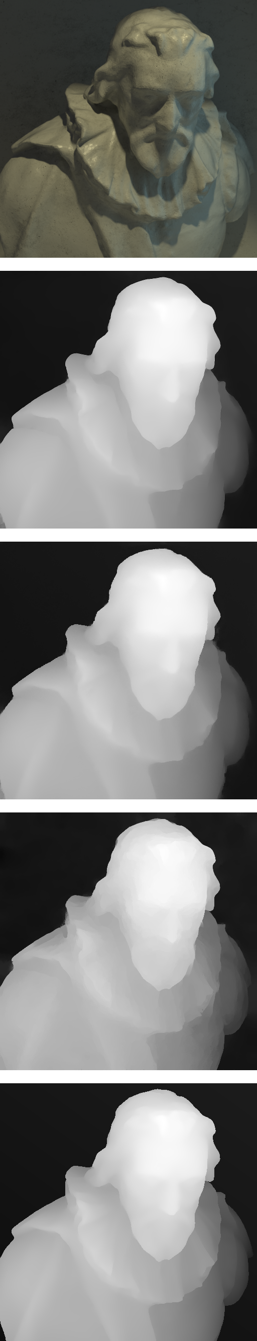
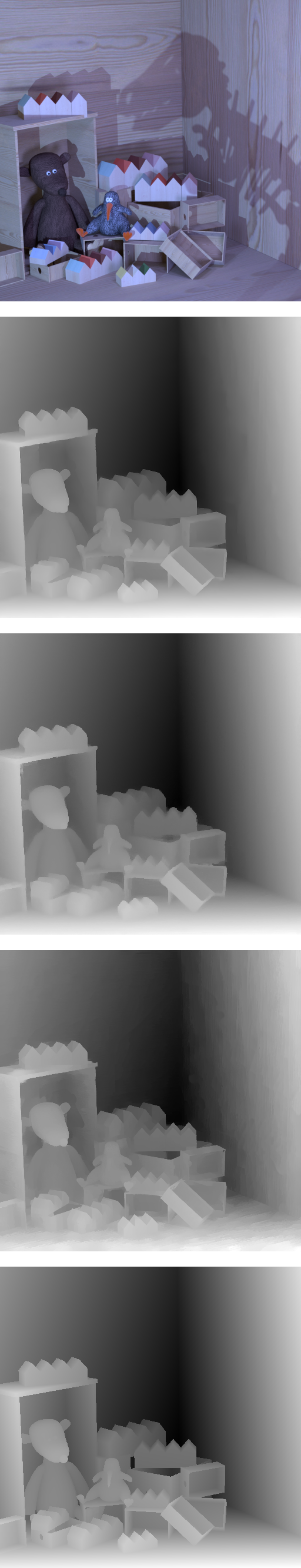
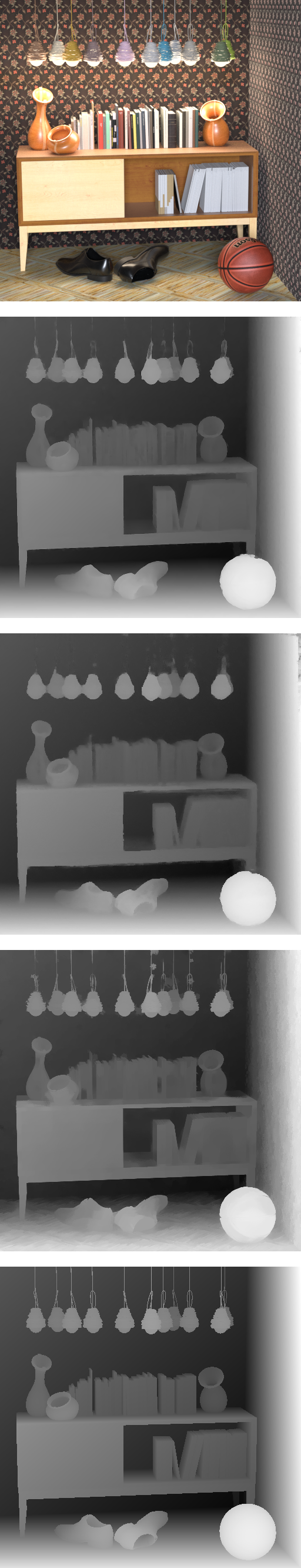
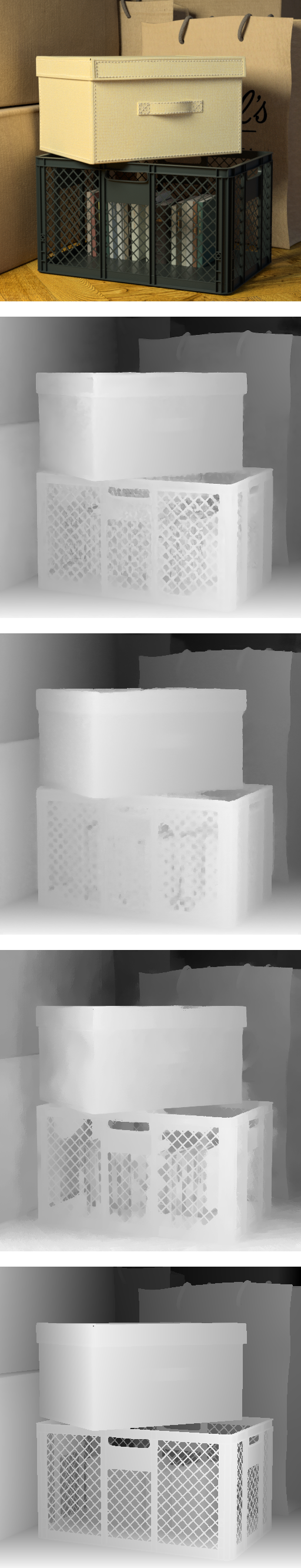
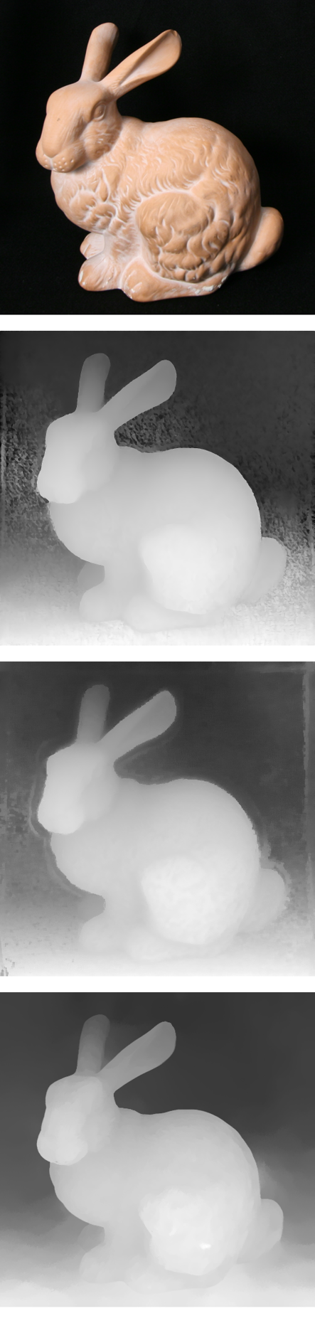
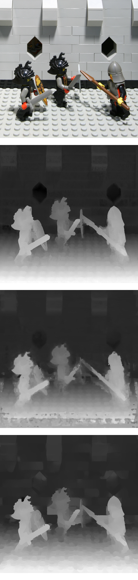
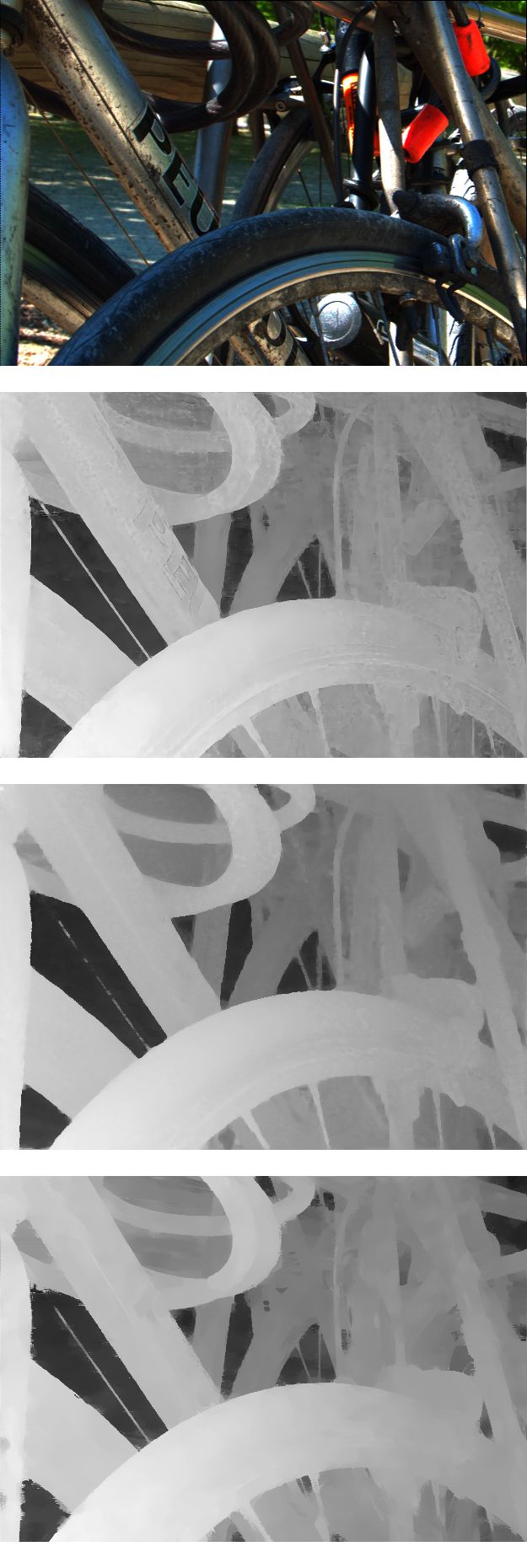
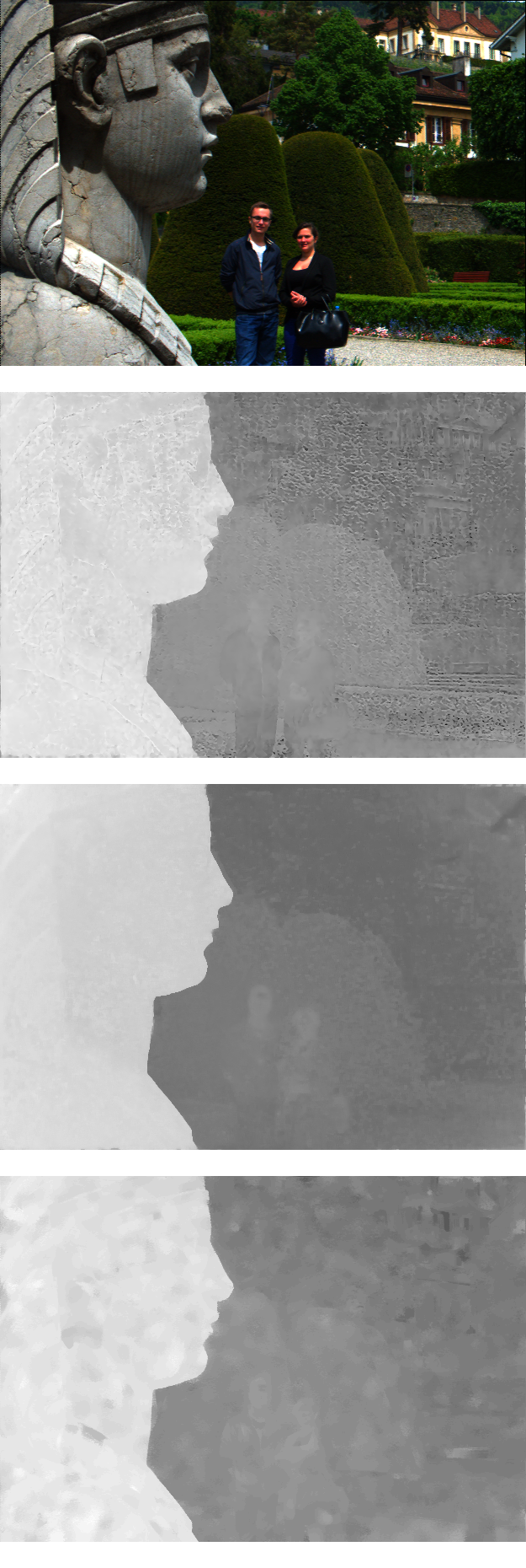
Qualitative
Figures 5 and 6 present qualitative single-view depth map results. To assess view consistency, we refer the reader to our supplemental video, which also includes accuracy error and view inconsistency heat map visualizations for all scenes. Overall, all methods produce broadly comparable results, though each method has different characteristics. The learning-based methods tend to produce smoother depths across flat regions. All methods struggle with thin features; our approach fares better with correct surrounding disocclusions (Boxes crate; see video). On the Bunny scene, our approach introduces fewer background errors and shows fewer ‘edging’ artifacts than Jiang et al. Shi et al. produces cleaner depth map appearance for Lego, but is view inconsistent. Jiang et al. is view consistent, but introduces artifacts on Lego. One limitation of our method is on Sphynx, where a distant scene and narrow baseline cause noise in our EPI line reconstruction.
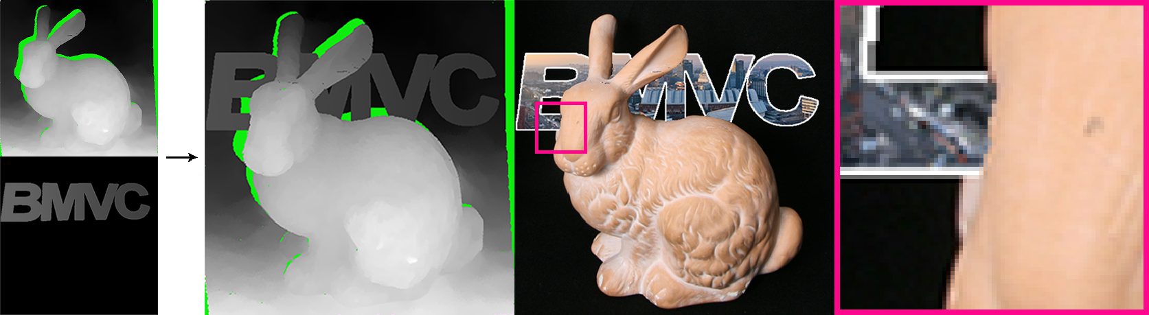
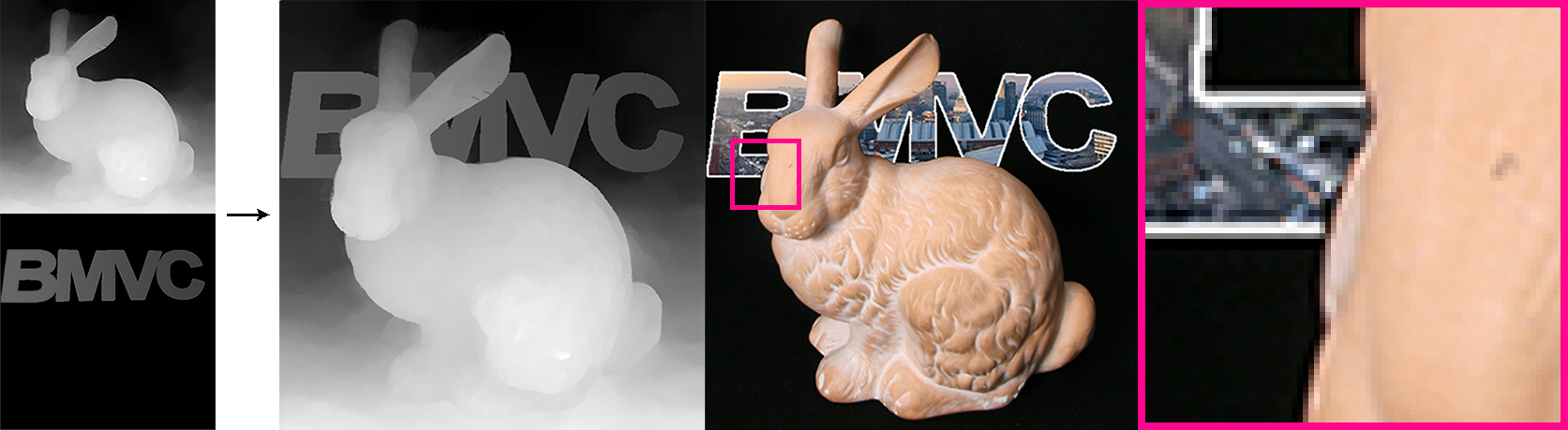
Applications
Consistent per-view disparity estimates are vital for practical applications such as light field editing: knowing the disparity of regions occluded in the central view allows view-consistent decals or objects to be inserted into the 3D scene (Figure 4). Moreover, without per-view disparity, users can only edit the central view as changes in other views cannot be propagated across views. This limits editing flexibility.
5 Discussion and Conclusion
Our work demonstrates that careful handling of depth edge estimation, occlusions, and view consistency can produce per-view disparity maps with comparable performance to state of the art learning-based methods in terms of average accuracy and view consistency. This can also lead to computation time performance gains.
Nonetheless, our method does have limitations; one area where our lack of explicit (u,v) regularization is sometimes a factor is in spatial edge consistency, e.g., for diagonal angles in non-cross-hair views. Adding additional regularization begins another trade-off between smoothness, accuracy, and computational cost. Further, our method is limited when an EPI contains an area enclosed by high gradient boundaries with no data term depth value in it, and disocclusion propagation can be attributed either to the foreground occluder or revealed background (e.g., Lego scene, arm of right-most character).
Accurate edge estimation and occlusion reasoning is still a core problem, and greater context may help. Future work might apply small targeted deep-learned priors for efficiency.
References
- [sta(2008)] The New Stanford Light Field Archive, 2008. URL http://lightfield.stanford.edu/.
- [Alperovich et al.(2018)Alperovich, Johannsen, and Goldluecke] A. Alperovich, O. Johannsen, and B. Goldluecke. Intrinsic light field decomposition and disparity estimation with a deep encoder-decoder network. In 26th European Signal Processing Conference (EUSIPCO), 2018.
- [Barnes et al.(2009)Barnes, Shechtman, Finkelstein, and Goldman] Connelly Barnes, Eli Shechtman, Adam Finkelstein, and Dan B Goldman. PatchMatch: A randomized correspondence algorithm for structural image editing. ACM Transactions on Graphics (Proc. SIGGRAPH), 28(3), August 2009.
- [Bhat et al.(2009)Bhat, Zitnick, Cohen, and Curless] Pravin Bhat, Larry Zitnick, Michael Cohen, and Brian Curless. Gradientshop: A gradient-domain optimization framework for image and video filtering. In ACM Transactions on Graphics (TOG), 2009.
- [Chen et al.(2018)Chen, Hou, Ni, and Chau] Jie Chen, Junhui Hou, Yun Ni, and Lap-Pui Chau. Accurate light field depth estimation with superpixel regularization over partially occluded regions. IEEE Transactions on Image Processing, 27(10):4889–4900, 2018.
- [Chuchvara et al.(2020)Chuchvara, Barsi, and Gotchev] A. Chuchvara, A. Barsi, and A. Gotchev. Fast and accurate depth estimation from sparse light fields. IEEE Transactions on Image Processing (TIP), 29:2492–2506, 2020.
- [Holynski and Kopf(2018)] Aleksander Holynski and Johannes Kopf. Fast depth densification for occlusion-aware augmented reality. In ACM Transactions on Graphics (Proc. SIGGRAPH Asia), volume 37. ACM, 2018.
- [Honauer et al.(2016)Honauer, Johannsen, Kondermann, and Goldluecke] Katrin Honauer, Ole Johannsen, Daniel Kondermann, and Bastian Goldluecke. A dataset and evaluation methodology for depth estimation on 4d light fields. In Asian Conference on Computer Vision, pages 19–34. Springer, 2016.
- [Huang et al.(2018)Huang, Matzen, Kopf, Ahuja, and Huang] Po-Han Huang, Kevin Matzen, Johannes Kopf, Narendra Ahuja, and Jia-Bin Huang. DeepMVS: Learning multi-view stereopsis. In IEEE Conference on Computer Vision and Pattern Recognition (CVPR), pages 2821–2830, 2018.
- [Ilg et al.(2017)Ilg, Mayer, Saikia, Keuper, Dosovitskiy, and Brox] Eddy Ilg, Nikolaus Mayer, Tonmoy Saikia, Margret Keuper, Alexey Dosovitskiy, and Thomas Brox. Flownet 2.0: Evolution of optical flow estimation with deep networks. In IEEE Conference on Computer Vision and Pattern Recognition (CVPR), pages 2462–2470, 2017.
- [Jeon et al.(2015)Jeon, Park, Choe, Park, Bok, Tai, and So Kweon] Hae-Gon Jeon, Jaesik Park, Gyeongmin Choe, Jinsun Park, Yunsu Bok, Yu-Wing Tai, and In So Kweon. Accurate depth map estimation from a lenslet light field camera. In IEEE Conference on Computer Vision and Pattern Recognition (CVPR), pages 1547–1555, 2015.
- [Jiang et al.(2018)Jiang, Le Pendu, and Guillemot] Xiaoran Jiang, Mikaël Le Pendu, and Christine Guillemot. Depth estimation with occlusion handling from a sparse set of light field views. In 25th IEEE International Conference on Image Processing (ICIP), pages 634–638. IEEE, 2018.
- [Jiang et al.(2019)Jiang, Shi, and Guillemot] Xiaoran Jiang, Jinglei Shi, and Christine Guillemot. A learning based depth estimation framework for 4d densely and sparsely sampled light fields. In Proceedings of the 44th International Conference on Acoustics, Speech, and Signal Processing (ICASSP), 2019.
- [Khan et al.(2019)Khan, Zhang, Kasser, Stone, Kim, and Tompkin] Numair Khan, Qian Zhang, Lucas Kasser, Henry Stone, Min H. Kim, and James Tompkin. View-consistent 4D light field superpixel segmentation. In International Conference on Computer Vision (ICCV). IEEE, 2019.
- [Khan et al.(2020)Khan, Kim, and Tompkin] Numair Khan, Min H. Kim, and James Tompkin. Fast and accurate 4D light field depth estimation. Technical Report CS-20-01, Brown University, 2020.
- [Ma et al.(2013)Ma, He, Wei, Sun, and Wu] Ziyang Ma, Kaiming He, Yichen Wei, Jian Sun, and Enhua Wu. Constant time weighted median filtering for stereo matching and beyond. In Proceedings of the IEEE International Conference on Computer Vision, pages 49–56, 2013.
- [Rerabek and Ebrahimi(2016)] Martin Rerabek and Touradj Ebrahimi. New light field image dataset. In 8th International Conference on Quality of Multimedia Experience (QoMEX), number CONF, 2016.
- [Shi et al.(2019)Shi, Jiang, and Guillemot] Jinglei Shi, Xiaoran Jiang, and Christine Guillemot. A framework for learning depth from a flexible subset of dense and sparse light field views. IEEE Transactions on Image Processing (TIP), 28(12):5867–5880, 2019.
- [Shih et al.(2020)Shih, Su, Kopf, and Huang] Meng-Li Shih, Shih-Yang Su, Johannes Kopf, and Jia-Bin Huang. 3d photography using context-aware layered depth inpainting. In IEEE Conference on Computer Vision and Pattern Recognition (CVPR), 2020.
- [Szeliski(2006)] Richard Szeliski. Locally adapted hierarchical basis preconditioning. In ACM SIGGRAPH 2006 Papers, pages 1135–1143. 2006.
- [Tao et al.(2013)Tao, Hadap, Malik, and Ramamoorthi] Michael W Tao, Sunil Hadap, Jitendra Malik, and Ravi Ramamoorthi. Depth from combining defocus and correspondence using light-field cameras. In IEEE International Conference on Computer Vision (ICCV), pages 673–680, 2013.
- [Tosic and Berkner(2014)] Ivana Tosic and Kathrin Berkner. Light field scale-depth space transform for dense depth estimation. In IEEE Conference on Computer Vision and Pattern Recognition Workshops (CVPRW), pages 435–442, 2014.
- [Wang et al.(2015)Wang, Efros, and Ramamoorthi] Ting-Chun Wang, Alexei A Efros, and Ravi Ramamoorthi. Occlusion-aware depth estimation using light-field cameras. In IEEE International Conference on Computer Vision (ICCV), pages 3487–3495, 2015.
- [Wang et al.(2016)Wang, Efros, and Ramamoorthi] Ting-Chun Wang, Alexei A Efros, and Ravi Ramamoorthi. Depth estimation with occlusion modeling using light-field cameras. IEEE Transactions on Pattern Analysis and Machine Intelligence (TPAMI), 38(11):2170–2181, 2016.
- [Wanner and Goldluecke(2012)] Sven Wanner and Bastian Goldluecke. Globally consistent depth labeling of 4d light fields. In IEEE Conference on Computer Vision and Pattern Recognition (CVPR), pages 41–48. IEEE, 2012.
- [Wanner and Goldluecke(2013)] Sven Wanner and Bastian Goldluecke. Variational light field analysis for disparity estimation and super-resolution. IEEE transactions on pattern analysis and machine intelligence, 36(3):606–619, 2013.
- [Zhang et al.(2016)Zhang, Sheng, Li, Zhang, and Xiong] Shuo Zhang, Hao Sheng, Chao Li, Jun Zhang, and Zhang Xiong. Robust depth estimation for light field via spinning parallelogram operator. Computer Vision and Image Understanding, 145:148–159, 2016.