This paper was converted on www.awesomepapers.org from LaTeX by an anonymous user.
Want to know more? Visit the Converter page.

Vertex Operators of the KP hierarchy and Singular Algebraic Curves

Atsushi Nakayashiki 111 Department of Mathematics, Tsuda University, Kodaira, Tokyo 187-8577, Japan, [email protected]
Abstract

Quasi-periodic solutions of the KP hierarchy acted by vertex operators are studied. We show, with the aid of the Sato Grassmannian, that solutions thus constructed correspond to torsion free rank one sheaves on some singular algebraic curves whose normalizations are the non-singular curves corresponding to the seed quasi-periodic solutions. It means that the action of the vertex operator has an effect of creating singular points on an algebraic curve. We further check, by examples, that solutions obtained here can be considered as solitons on quasi-periodic backgrounds, where the soliton matrices are deterimed by parameters in the vertex operators.

1 Introduction

We revisit the vertex operators of the KP-hierarchy [5]. We apply them to quasi-periodic solutions, that is, solutions which are expressed by Riemann’s theta functions of non-singular algebraic curves [22]. The problem we consider here is what kind of solutions we get in this way. To study this problem we use the Sato Grassmannian [36]. We show that solutions obatined here correspond to certain singular algebraic curves whose normalizations are the non-singular curves of the seed quasi-periodic solutions. It implies two things. First is that the action of the vertex operator of the KP-hierarchy has the effect of creating certain singularities on a curve. Second is that the solutions created by vertex operators describe certain limits of quasi-periodic solutions, since singular curves may be considered as limits of non-singular curves. We check, by computer simulations, that the solutions here represent solitons on the quasi-periodic backgrounds, where the soliton matrices can be extracted from the parameters of the vertex operators. It implies that wave patterns of quasi-periodic solutions of the KP equation contain various shapes of soliton solutions [16, 17] as a part. Recently interactions of solitons and quasi-periodic solutions attracted much attention in relation with soliton gases [10, 18, 7]. It is interesting to study whether the results in this paper can have some application to this subject.

Now let us explain the results in more detail along the history of researches. During the last two decades it is revealed that the shapes of soliton solutions of the KP equation form various wave patterns like web diagrams [4, 16, 17]. Those wave patterns are related with combinatorics of non-negative Grassmannians and cluster algebras [20, 21]. Mathematically soliton solutions, in terms of tau function, are those described by linear combinations of exponential functions and are known to be constructed from singular algebraic curves of genus 0 [23, 38]. Quasi-periodic solutions of the KP equation are those written by Riemann’s theta function of non-singular algebraic curves of positive genus [22, 37]. It is expected that quasi-periodic solutions tend to soliton solutions in certain genus zero limits [23, 38, 1]. Therefore it is quite interesting to study the wave patterns of quasi-periodic solutions incorporating the recent development on soliton solutions.

One strategy to study this problem is to take limits of quasi-periodic solutions and make correspondence between quasi-periodic solutions and soliton solutions. However, to carry out this program was not very easy because it is difficult to compute limits of period matrices. We have avoided this difficulty by using the Sato Grassmannian and have calculated limits of quasi-periodic solutions for several examples [31, 32, 33, 34]. Recently there are important progress in computing the limits of quasi-periodic solutions [2, 3, 12, 11]. In [12], in particular, some kind of limits have been computed for any Riemann surface. However it seems difficult to understand how solitonic structure is incorporated in the wave patterns of quasi-periodic solutions from those results.

In this paper we change the direction of study. Instead of studying the limits of quasi-periodic solutions we construct solutions corresponding to degenerate algebraic curves which are more covenient to see the relation with soliton solutions. In course of studying the degeneration of quasi-periodic solutions we found the following formula (Theorem 4.5 of [33] ):

limτg,0(t)=Ce2l=1αlt2l\displaystyle\lim\tau_{g,0}(t)=C{\rm e}^{-2\sum_{l=1}^{\infty}\alpha^{l}t_{2l}}
×(eη(t,α1/2)τg1,0(t[α1/2])+(1)neη(t,α1/2)τg1,0(t[α1/2])),\displaystyle\times\Bigl{(}{\rm e}^{\eta(t,\alpha^{1/2})}\tau_{g-1,0}(t-[\alpha^{-1/2}])+(-1)^{n}{\rm e}^{\eta(t,-\alpha^{1/2})}\tau_{g-1,0}(t-[-\alpha^{-1/2}])\Bigr{)},

where CC is a certain constant, t=(t1,t2,t3,)t=(t_{1},t_{2},t_{3},...), [κ]=(κ,κ2/2,κ3/3,)[\kappa]=(\kappa,\kappa^{2}/2,\kappa^{3}/3,...), η(t,p)=j=1tjpj\eta(t,p)=\sum_{j=1}^{\infty}t_{j}p^{j}, τn,0\tau_{n,0} is a quasi-periodic solution of the KdV hierarchy, expressed in some standard form, corresponding to a hyperelliptic curve of genus nn, lim means pinching a pair of branching points and α\alpha is the parameter correponding to the pinched point. The term inside the bracket of the right hand side has a very special form. It is rewritten using the vertex operator introduced in [5]:

X(p,q)=eη(t,p)η(t,q)eη(~,p1)+η(~,q1),\displaystyle X(p,q)=e^{\eta(t,p)-\eta(t,q)}e^{-\eta(\tilde{\partial},p^{-1})+\eta(\tilde{\partial},q^{-1})},
~=(1,2/2,3/3,).\displaystyle\tilde{\partial}=(\partial_{1},\partial_{2}/2,\partial_{3}/3,...).

In fact, for any function τ(t)\tau(t), we have

eη(t,q)eaX(p,q)τ(t[q1])=eη(t,q)τ(t[q1])+aeη(t,p)τ(t[p1]).\displaystyle e^{\eta(t,q)}e^{aX(p,q)}\tau(t-[q^{-1}])=e^{\eta(t,q)}\tau(t-[q^{-1}])+ae^{\eta(t,p)}\tau(t-[p^{-1}]).

If we take (p,q)=(α1/2,α1/2)(p,q)=(-\alpha^{1/2},\alpha^{1/2}), a=(1)na=(-1)^{n} and τ(t)=τg1,0\tau(t)=\tau_{g-1,0}, we recover the above formula. The vertex operator transforms a solution of the KP-hierarchy to another one, that is, if τ(t)\tau(t) is a solution then eaX(p,q)τ(t)e^{aX(p,q)}\tau(t) is again a solution for any constant aa [5]. The above fact suggests that the limits of quasi-periodic solutions may be described by the action of vertex operators on quasi-periodic solutions. The aim of this paper is, in a sense, to show that this is actually the case.

Let τ0(t)\tau_{0}(t) be the quasi-periodic solution of the KP-hierarchy constructed from the data (C,LΔ,e,p,z)(C,L_{\Delta,e},p_{\infty},z), where CC is a compact Riemann surface of genus g>0g>0, LΔ,eL_{\Delta,e} is a certain holomorphic line bundle on CC of degree g1g-1, pp_{\infty} a point of CC and zz is a local coordinate around pp_{\infty} [22, 37, 15]. We apply vertex operators with various parameters successively to τ0(t)\tau_{0}(t). More precisely, let M,N1M,N\geq 1, pi,qjp_{i},q_{j}, 1iN1\leq i\leq N, 1jM1\leq j\leq M distinct complex parameters, A=(ai,j)A=(a_{i,j}) an M×NM\times N matrix. We consider the vertex operator of the form

G=ei=1Mj=1Nai,jX(qi1,pj1).\displaystyle G=e^{\sum_{i=1}^{M}\sum_{j=1}^{N}a_{i,j}X(q_{i}^{-1},p_{j}^{-1})}.

We make a certain shift on τ0(t)\tau_{0}(t), apply GG and multiply it by a constant times exponential function and a get new solution τ(t)\tau(t) (cf. (3.3)). We show that τ(t)\tau(t) is a solution constructed from the data (C,𝒲e,p,z)(C^{\prime},{\cal W}_{e},p^{\prime}_{\infty},z) where CC^{\prime} is a certain singular algebraic curve whose normalization is CC, 𝒲e{\cal W}_{e} is a certain torsion free sheaf of rank one on CC^{\prime} , pp^{\prime}_{\infty} is a point of CC^{\prime} and zz a local coordinate around pp^{\prime}_{\infty}. To prove these properties we use the Sato Grassmannian, which we denote by UGM. It is the set of certain subspaces of the vector space V=((z))V=\mathbb{C}((z)) and parametrizes all formal power solutions of the KP-hierarchy. We recall here that if τ(t)\tau(t) is a solution of the KP-hierarchy so is τ(t)\tau(-t). W remark that the descriptions of the points of UGM corresponding to τ(t)\tau(t) and τ(t)\tau(-t) are not very symmetric. The point corresponding to τ(t)\tau(-t) is more suitable to describe the geometry. By this reason we determine the point WeW_{e} of UGM corresponding to τ(t)\tau(-t). This is done by examining the properties of the wave function associated with τ(t)\tau(t) (cf. (2.4)).

The subspace of VV corresponding to τ0(t)\tau_{0}(-t) is a module over the affine coordinate ring RR of C\{p}C\backslash\{p_{\infty}\}. Since WeW_{e} is a subspace of this space, we consider the stabilizer ReR_{e} of WeW_{e} in RR. Following Mumford [27] and Mulase[25, 26] we define CC^{\prime}and 𝒲e{\cal W}_{e} as a scheme and a sheaf on it respectively using ReR_{e} and WeW_{e}.

Finally it should be mentioned that the relation of the vertex operator and the degeneration of Riemann’s theta function has also been observed by Yuji Kodama from different point of view [18, 19]. It is interesting to investigate the relation of the results of this paper and those of Kodama.

The paper is organized as follows. In section 2 the relation of the KP-hierarchy and the Sato Grassmannian is reviewed. The main results are formulated and stated in section 3. The formula for a quasi-periodic solution, the definition and the properties of the vertex operator and the result of the action of the vertex operator on a quasi-periodic solution are given here. In section 4 the singular algebraic curve and the sheaf on it associated with the solution considered in the main theorem are defined and their properties are studied. The example of genus one is studied in detal in section 5. Figures of computer simulation by Mathematica are presented here. The proof of the main theorem is given in section 4 and 5. Regarding the readability of the paper proofs of assertions in section 4 are given in appendix A to E.

2 KP-hierarchy and Sato Grassmannian

The KP-hierarchy is the equation for a function τ(t)\tau(t), t=(t1,t2,t3,)t=(t_{1},t_{2},t_{3},...) of the form

τ(ts[λ1])(t+s+[λ1])e2η(s,λ)dλ2πi=0,\displaystyle\oint\tau(t-s-[\lambda^{-1}])(t+s+[\lambda^{-1}])e^{-2\eta(s,\lambda)}\frac{d\lambda}{2\pi i}=0, (2.1)

where s=(s1,s2,s3,)s=(s_{1},s_{2},s_{3},...),

[μ]=(μ,μ22,μ33,),η(t,λ)=n=1tnλn,\displaystyle[\mu]=(\mu,\frac{\mu^{2}}{2},\frac{\mu^{3}}{3},...),\hskip 14.22636pt\eta(t,\lambda)=\sum_{n=1}^{\infty}t_{n}\lambda^{n},

and dλ2πi\oint\cdot\frac{d\lambda}{2\pi i} means taking the residue at λ=\lambda=\infty. By expanding in {sj}\{s_{j}\} the KP-hierarchy is equivalent to the infinite set of differential equations which include the KP equation in the bilinear form:

(D143D224D1D3)ττ=0,\displaystyle(D_{1}^{4}-3D_{2}^{2}-4D_{1}D_{3})\tau\cdot\tau=0, (2.2)

where the Hirota derivatives DiD_{i} is defined, in general, for a function f(t)f(t), as the Taylor coefficients of the expansion of f(t+s)f(ts)f(t+s)f(t-s) in ss:

f(t+s)f(ts)=Dαffα!sα,\displaystyle f(t+s)f(t-s)=\sum\frac{D^{\alpha}f\cdot f}{\alpha!}s^{\alpha},

where α=(α1,α2,)\alpha=(\alpha_{1},\alpha_{2},...), Dα=D1α1D2α2D^{\alpha}=D_{1}^{\alpha_{1}}D_{2}^{\alpha_{2}}\cdots, α!=α1!α2!\alpha!=\alpha_{1}!\alpha_{2}!\cdots, sα=s1α1s2α2s^{\alpha}=s_{1}^{\alpha_{1}}s_{2}^{\alpha_{2}}\cdots. If x=t1x=t_{1}, y=t2y=t_{2}, t=t3t=t_{3} and u=2x2logτ(t)u=2\partial_{x}^{2}\log\tau(t), (2.2) implies the KP equation

3uyy+(4ut+6uux+uxxx)x=0.\displaystyle 3u_{yy}+(-4u_{t}+6uu_{x}+u_{xxx})_{x}=0. (2.3)

The Sato Grassmannian, which we denote by UGM after Sato, parametrizes all formal power series solutions of the KP-hierarchy. It is defined as follows.

Let V=((z))V={\mathbb{C}}((z)) be the space of formal Laurent series in one variable zz, Vϕ=[z1]V_{\phi}={\mathbb{C}}[z^{-1}] the subspace of polynomials in z1z^{-1} and V0=z[[z]]V_{0}=z{\mathbb{C}}[[z]] the subspace of formal power series vanishing at z=0z=0. Then V=VϕV0V=V_{\phi}\oplus V_{0}. The Sato Grassmannian is the set of subspaces of VV with the same size as VϕV_{\phi}. More precisely let π:VVϕ\pi:V\rightarrow V_{\phi} be the projection. Then UGM is the set of a subspace UU such that Kerπ|U{\rm Ker}\pi|_{U} and Cokerπ|U{\rm Coker}\pi|_{U} is both finite dimensional and their dimensions are same.

Here we shall give a criterion for a subspace of VV to be a point of UGM. To this end, for f(z)Vf(z)\in V, define the order of ff by,

ordf=N if f(z)=czN+O(zN+1) with c0.\displaystyle\operatorname{ord}f=-N\text{ if $f(z)=cz^{N}+O(z^{N+1})$ with $c\neq 0$.}

It describes the order of a pole at z=0z=0 if NN is negative. We set

V(n)={fV|ordfn},\displaystyle V(n)=\{f\in V\,|\,\operatorname{ord}f\leq n\},

and, for a subspace UU of VV, set U(n)=UV(n)U(n)=U\cap V(n). Then

Proposition 2.1.

A subspace UU of VV belongs to UGM if and only if dimU(n)=n+1\dim U(n)=n+1 for all sufficiently large nn.

Proof. Suppose that dimU(n)=n+1\dim U(n)=n+1 for nn0n\geq n_{0} with n00n_{0}\geq 0. Then dimU(n+1)/U(n)=1\dim U(n+1)/U(n)=1 for nn0n\geq n_{0}. It means that there exist fnUf_{n}\in U, nn0+1n\geq n_{0}+1, such that

fn=zn+O(zn+1),nn0+1.\displaystyle f_{n}=z^{-n}+O(z^{-n+1}),\hskip 14.22636ptn\geq n_{0}+1.

We can take fnf_{n}, nn0+1n\geq n_{0}+1, as a part of a basis of UU. For the remaining part, since dimU(n0)=n0+1\dim U(n_{0})=n_{0}+1, there exist fmiUf_{m_{i}}\in U, 0in00\leq i\leq n_{0} such that ordfmi=mi\operatorname{ord}f_{m_{i}}=m_{i} with m0<<mn0m_{0}<\cdots<m_{n_{0}}. By the definition

r:=dimKerπ|U={j|mj<0}.\displaystyle r:=\dim{\rm Ker}\pi|_{U}=\sharp\{j\,|\,m_{j}<0\}.

Then

dimCokerπ|U=n0+1(n0+1r)=r.\displaystyle\dim{\rm Coker}\pi|_{U}=n_{0}+1-(n_{0}+1-r)=r.

Thus UUGMU\in UGM. ∎

Corollary 2.2.

Let WW be a subspace of VV. If there exists an integer NN such that dimW(n)=nN\dim W(n)=n-N for all sufficiently large nn, then U=zN+1WU=z^{N+1}W is a point of UGM.

Proof. Since U(n)=zN+1W(n+N+1)U(n)=z^{N+1}W(n+N+1) and therefore dimU(n)=dimW(n+N+1)=n+1\dim U(n)=\dim W(n+N+1)=n+1 for sufficiently large nn. Thus the assertion follows from Proposition 2.1. ∎


Example 2.3.

W=z3+z2+i=4zi\displaystyle W={\mathbb{C}}z^{3}+{\mathbb{C}}z^{2}+\sum_{i=4}^{\infty}{\mathbb{C}}z^{-i}. For n4n\geq 4 dimW(n)=n1\dim W(n)=n-1. Then U=z2W=z5+z4+i=2zi\displaystyle U=z^{2}W={\mathbb{C}}z^{5}+{\mathbb{C}}z^{4}+\sum_{i=2}^{\infty}{\mathbb{C}}z^{-i} is a point of UGM since Kerπ|U=z5+z4{\rm Ker}\pi|_{U}={\mathbb{C}}z^{5}+{\mathbb{C}}z^{4} and Cokerπ|U=1+z1{\rm Coker}\pi|_{U}={\mathbb{C}}1+{\mathbb{C}}z^{-1}.

Next we explain the correspondence between solutions of the KP-hierarchy and points of UGM. For a point of UGM the corresponding solution of the KP-hierarchy is constructed as a series using Schur functions and Plücker coordinates. For this see [32].

We need, in this paper, the converse construction of the point of UGM from a solution of the KP-hierarchy. Let τ(t)\tau(t) be a solution of the KP-hierarchy. Define the wave function Ψ(t;z)\Psi(t;z) and the adjoint wave function Ψ(t;z)\Psi^{\ast}(t;z) by

Ψ(t;z)=τ(t[z])τ(t)eη(t,z1),Ψ(t;z)=τ(t+[z])τ(t)eη(t,z1).\displaystyle\Psi(t;z)=\frac{\tau(t-[z])}{\tau(t)}e^{\eta(t,z^{-1})},\hskip 28.45274pt\Psi^{\ast}(t;z)=\frac{\tau(t+[z])}{\tau(t)}e^{-\eta(t,z^{-1})}. (2.4)
Theorem 2.4.

[36, 15] Let UU be the vector space spanned by the expansion coefficients of τ(t)Ψ(t;z)\tau(t)\Psi^{\ast}(t;z) in tt. Then UU is the point of UGM corresponding to τ(t)\tau(t).

It is easy to verify that if τ(t)\tau(t) is a solution of the KP-hierarchy so is τ(t)\tau(-t).

Corollary 2.5.

Let UU^{\prime} be the vector space spanned by the expansion coefficients of τ(t)Ψ(t;z)\tau(t)\Psi(t;z) in tt Then UU^{\prime} is the point of UGM corresponding to τ(t)\tau(-t).

Proof. Let Ψ(t;z)\Psi_{-}^{\ast}(t;z) be the adjoint wave function of τ(t)\tau(-t). Then

τ(t)Ψ(t;z)=τ(t[z])eη(t,z1).\displaystyle\tau(-t)\Psi_{-}^{\ast}(t;z)=\tau(-t-[z])e^{-\eta(t,z^{-1})}. (2.5)

If we set s=ts=-t, it is equal to

τ(s[z])eη(s,z1)=τ(s)Ψ(s;z).\displaystyle\tau(s-[z])e^{\eta(s,z^{-1})}=\tau(s)\Psi(s;z). (2.6)

Since the vector space generated by the expansion coefficients of (2.6) in ss is the same as that generated by expansion coefficients of (2.5) in tt, the assertion of the lemma follows from Theorem 2.4. ∎

3 Main results

Let CC be a compact Riemann surface of genus g>0g>0, {αi,βi}i=1g\{\alpha_{i},\beta_{i}\}_{i=1}^{g} a canonical basis of H1(C,)H^{1}(C,{\mathbb{Z}}), {dvi}i=1g\{dv_{i}\}_{i=1}^{g} the normalized basis of holomorphic one forms, Ω=(Ωi,j)1i,jg\Omega=(\Omega_{i,j})_{1\leq i,j\leq g} with Ωi,j=βj𝑑vi\Omega_{i,j}=\int_{\beta_{j}}dv_{i} the period matrix, J(C)=g/LΩJ(C)={\mathbb{C}}^{g}/L_{\Omega} with LΩ=g+ΩgL_{\Omega}={\mathbb{Z}}^{g}+\Omega{\mathbb{Z}}^{g} the Jacobian variety of CC, pp_{\infty} a point of CC, I(p)=pp𝑑vI(p)=\int_{p_{\infty}}^{p}dv with dv=(dv1,,dvg)tdv={}^{t}(dv_{1},...,dv_{g}) the Abel map, KK Riemann’s constant, θ(z|Ω)\theta(z|\Omega) Riemann’s theta function

θ(z|Ω)=ngexp(πintΩn+2πintz),z=(z1,,zg)t,\displaystyle\theta(z|\Omega)=\sum_{n\in{\mathbb{Z}}^{g}}\exp(\pi i{}^{t}n\Omega n+2\pi i{}^{t}nz),\quad z={}^{t}(z_{1},...,z_{g}),

where ngn\in{\mathbb{Z}}^{g} is considered as a column vector.

We extend the the definition of the Abel map to divisors of any degree by, for D=j=1mpjj=1nqj\displaystyle D=\sum_{j=1}^{m}p_{j}-\sum_{j=1}^{n}q_{j},

I(D)=j=1mI(pj)j=1nI(qj).\displaystyle I(D)=\sum_{j=1}^{m}I(p_{j})-\sum_{j=1}^{n}I(q_{j}).

We denote by Δ\Delta the Riemann divisor. It is the dvisor of degree g1g-1 which satisfies 2ΔΩC12\Delta\equiv\Omega_{C}^{1} and I(Δ)=KI(\Delta)=K, where \equiv signifies the linear equivalence of divisors and ΩC1\Omega^{1}_{C} is the linear equivalence class of divisors of holomorphic one forms. The Riemann divisor is uniquely determined from the canonical homology basis by the condition [28]

{I(p1++pg1Δ)|p1,,pg1C}={zJ(C)|θ(z|Ω)=0}.\displaystyle\{I(p_{1}+\cdots+p_{g-1}-\Delta)\,|\,p_{1},...,p_{g-1}\in C\}=\{z\in J(C)\,|\,\theta(z|\Omega)=0\}.

Notice that the left hand side does not depend on the choice of the base point pp_{\infty} of the Abel map.

Let E(p1,p2)E(p_{1},p_{2}) be the prime form [8, 29] (see also [30]):

E(p1,p2)=θ[δ](p1p2𝑑v)hδ(p1)hδ(p2),\displaystyle E(p_{1},p_{2})=\frac{\theta[\delta](\int_{p_{1}}^{p_{2}}dv)}{h_{\delta}(p_{1})h_{\delta}(p_{2})},

where δ=(δδ′′)\delta=\binom{\delta^{\prime}}{\delta^{\prime\prime}}, δ,δ′′12g\delta^{\prime},\delta^{\prime\prime}\in\frac{1}{2}{\mathbb{Z}}^{g} is a non-singular odd half characteristic and hδ(p)h_{\delta}(p) is the half differential satisfying

hδ2(p)=j=1gθ[δ]zj(0)dvj(p).\displaystyle h_{\delta}^{2}(p)=\sum_{j=1}^{g}\frac{\partial\theta[\delta]}{\partial z_{j}}(0)dv_{j}(p).

Take a local coordinate zz around pp_{\infty} and write

E(P1,P2)=E(z1,z2)dz1dz2,PiC,zi=z(Pi),\displaystyle E(P_{1},P_{2})=\frac{E(z_{1},z_{2})}{\sqrt{dz_{1}}\sqrt{dz_{2}}},\hskip 14.22636ptP_{i}\in C,\quad z_{i}=z(P_{i}),
dz1dz2logE(z1,z2)=(1(z1z2)2+i,j=1qi,jz1i1z2j1)dz1dz2,\displaystyle d_{z_{1}}d_{z_{2}}\log E(z_{1},z_{2})=\left(\frac{1}{(z_{1}-z_{2})^{2}}+\sum_{i,j=1}^{\infty}q_{i,j}z_{1}^{i-1}z_{2}^{j-1}\right)dz_{1}dz_{2}, (3.1)
dvi=j=1vi,jzj1dz.\displaystyle dv_{i}=\sum_{j=1}^{\infty}v_{i,j}z^{j-1}dz.

We set

𝒱=(vi,j)1ig,1j,q(t)=i,j=1qi,jtitj.\displaystyle{\cal V}=(v_{i,j})_{1\leq i\leq g,1\leq j},\hskip 28.45274ptq(t)=\sum_{i,j=1}^{\infty}q_{i,j}t_{i}t_{j}.

Then

τ0(t)=e12q(t)θ(𝒱t+e|Ω)\displaystyle\tau_{0}(t)=e^{\frac{1}{2}q(t)}\theta({\cal V}t+e|\Omega)

is a solution of the KP-hierarchy for arbitrary ege\in{\mathbb{C}}^{g} [37](see also [35, 15, 30]).

Let

X(p,q)=eη(t,p)η(t,q)eη(~,p1)+η(~,q1),\displaystyle X(p,q)=e^{\eta(t,p)-\eta(t,q)}e^{-\eta(\tilde{\partial},p^{-1})+\eta(\tilde{\partial},q^{-1})},
η(t,p)=j=1tjpj,~=(1,2/2,3/3,),\displaystyle\eta(t,p)=\sum_{j=1}^{\infty}t_{j}p^{j},\hskip 28.45274pt\tilde{\partial}=(\partial_{1},\partial_{2}/2,\partial_{3}/3,...),

be the vertex operator.

The following theorem is known.

Theorem 3.1.

[5] If τ(t)\tau(t) is a solution of the KP-hierarchy, so is eaX(p,q)τ(t)e^{aX(p,q)}\tau(t) for any aa\in{\mathbb{C}}.

Vertex operators satisfy

X(p1,q1)X(p2,q2)=(p1p2)(q1q2)(p1q2)(q1p2):X(p1,q1)X(p2,q2):\displaystyle X(p_{1},q_{1})X(p_{2},q_{2})=\frac{(p_{1}-p_{2})(q_{1}-q_{2})}{(p_{1}-q_{2})(q_{1}-p_{2})}:X(p_{1},q_{1})X(p_{2},q_{2}): (3.2)

where :::\quad: denotes the normal ordering taking all differential operators to the right of all multiplication operators, that is,

:X(p1,q1)X(p2,q2):=ej=12(η(t,pj)η(t,qj))ej=12(η(~,pj1)+η(~,qj1)).\displaystyle:X(p_{1},q_{1})X(p_{2},q_{2}):=e^{\sum_{j=1}^{2}(\eta(t,p_{j})-\eta(t,q_{j}))}e^{\sum_{j=1}^{2}(-\eta(\tilde{\partial},p_{j}^{-1})+\eta(\tilde{\partial},q_{j}^{-1}))}.

The following properties follow from this.

X(p1,q1)X(p2,q2)\displaystyle X(p_{1},q_{1})X(p_{2},q_{2}) =\displaystyle= X(p2,q2)X(p1,q1)if p1q2 and q1p2,\displaystyle X(p_{2},q_{2})X(p_{1},q_{1})\quad\text{if $p_{1}\neq q_{2}$ and $q_{1}\neq p_{2}$,}
X(p1,q1)X(p2,q2)\displaystyle X(p_{1},q_{1})X(p_{2},q_{2}) =\displaystyle= 0if p1=p2 or q1=q2.\displaystyle 0\quad\text{if $p_{1}=p_{2}$ or $q_{1}=q_{2}$}.

Let M,NM,N be positive integers, qiq_{i}, 1iM1\leq i\leq M, pjp_{j}, 1jN1\leq j\leq N non-zero complex numbers and (ai,j)(a_{i,j}) an M×NM\times N complex matrix. We set pN+j=qjp_{N+j}=q_{j} and use both notation pN+jp_{N+j} and qjq_{j}.

Set

G=ei=1Mj=1Nai,jX(qi1,pj1).\displaystyle G=e^{\sum_{i=1}^{M}\sum_{j=1}^{N}a_{i,j}X(q_{i}^{-1},p_{j}^{-1})}.

Define

τ(t)=Δ(p11,,pN1)ej=1Nη(t,pj1)Gτ0(tj=1N[pj]),\displaystyle\tau(t)=\Delta(p_{1}^{-1},...,p_{N}^{-1})e^{\sum_{j=1}^{N}\eta(t,p_{j}^{-1})}G\,\tau_{0}(t-\sum_{j=1}^{N}[p_{j}]), (3.3)

where Δ(p1,,pn)=1i<jn(pjpi)\Delta(p_{1},...,p_{n})=\prod_{1\leq i<j\leq n}(p_{j}-p_{i}). It can be computed explicitly as follows.

Set L=M+NL=M+N and define the L×NL\times N matrix B=(bi,j)B=(b_{i,j}) by

bi,j\displaystyle b_{i,j} =\displaystyle= δi,jfor 1i,jN,\displaystyle\delta_{i,j}\quad\text{for $1\leq i,j\leq N$},
bN+i,j\displaystyle b_{N+i,j} =\displaystyle= ai,jmjNpj1pm1qi1pm1for 1iM1jN,\displaystyle a_{i,j}\prod_{m\neq j}^{N}\frac{p_{j}^{-1}-p_{m}^{-1}}{q_{i}^{-1}-p_{m}^{-1}}\quad\text{for $1\leq i\leq M$, $1\leq j\leq N$}, (3.4)

that is,

B=(11bN+1,1bN+1,NbN+M,1bN+M,N).\displaystyle B=\left(\begin{array}[]{ccc}1&&\\ &\ddots&\\ &&1\\ b_{N+1,1}&\cdots&b_{N+1,N}\\ \vdots&&\vdots\\ b_{N+M,1}&\cdots&b_{N+M,N}\\ \end{array}\right). (3.11)

We set [L]={1,,L}[L]=\{1,...,L\} and denote by ([L]N)\binom{[L]}{N} the set of (i1,,iN)(i_{1},...,i_{N}), 1i1<<iNL1\leq i_{1}<\cdots<i_{N}\leq L [16, 17]. For I=(i1,,iN)([L]N)I=(i_{1},...,i_{N})\in\binom{[L]}{N} set

ΔI=Δ(pi11,,piN1),ηI=iIη(t,pi1),[pI]=iI[pi],\displaystyle\Delta^{-}_{I}=\Delta(p_{i_{1}}^{-1},...,p_{i_{N}}^{-1}),\hskip 14.22636pt\eta_{I}=\sum_{i\in I}\eta(t,p_{i}^{-1}),\hskip 14.22636pt[p_{I}]=\sum_{i\in I}[p_{i}],
BI=det(bir,s)1r,sN.\displaystyle B_{I}=\det(b_{i_{r},s})_{1\leq r,s\leq N}.

By a direct calculation using the commutation relation (3.2) we have

Proposition 3.2.

[34] The function τ(t)\tau(t) of (3.3) has the following expression

τ(t)=I([L]N)BIΔIeηIτ0(t[pI]).\displaystyle\tau(t)=\sum_{I\in\binom{[L]}{N}}B_{I}\Delta^{-}_{I}e^{\eta_{I}}\tau_{0}(t-[p_{I}]). (3.12)
Remark 3.3.

The matrices (ai,j)(a_{i,j}) and BB correspond to each other. When we study the positivity of τ(t)\tau(t), it is convenient to begin with the matrix BB and define the matrix (ai,j)(a_{i,j}) from it. For example, in the case where τ0(t)>0\tau_{0}(t)>0 for any real tt, {pi}\{p_{i}\} are real and p11<<pL1p_{1}^{-1}<\cdots<p_{L}^{-1}, then τ(t)>0\tau(t)>0 if BI0B_{I}\geq 0 for any II. Later in section 5 this view point is used.

The part τ0(t[pI])\tau_{0}(t-[p_{I}]) can further be expressed by theta function. To write it let dr~kd\tilde{r}_{k}, k1k\geq 1, be the normalized differential of the second kind with a pole only at pp_{\infty} of order k+1k+1, that is, it satisfies

αj𝑑r~k=0 for any j,dr~k=d(zkO(z)) near p.\displaystyle\int_{\alpha_{j}}d\tilde{r}_{k}=0\text{ for any $j$},\hskip 14.22636ptd\tilde{r}_{k}=d\left(z^{-k}-O(z)\right)\text{ near $p_{\infty}$}.

The expansion of dr~kd\tilde{r}_{k} near pp_{\infty} can be written more explicitly using {qi,j}\{q_{i,j}\}. In integral form it is given by

p𝑑r~k=zkj=1qk,jzjj,pC,z=z(p).\displaystyle\int^{p}d\tilde{r}_{k}=z^{-k}-\sum_{j=1}^{\infty}q_{k,j}\frac{z^{j}}{j},\hskip 14.22636ptp\in C,z=z(p). (3.13)

Then

Proposition 3.4.

In terms of the theta function τ(t)\tau(t) defined by (3.3) is written as

τ(t)=e12q(t)J([L]N)BJCJejJk=1tkPj𝑑r~kθ(𝒱tjJI(Qj)+e),\displaystyle\tau(t)=e^{\frac{1}{2}q(t)}\sum_{J\in\binom{[L]}{N}}B_{J}C_{J}e^{\sum_{j\in J}\sum_{k=1}^{\infty}t_{k}\int^{P_{j}}d\tilde{r}_{k}}\,\,\theta\left({\cal V}t-\sum_{j\in J}I(Q_{j})+e\right), (3.14)

where

CJ=i<j,i,jJE(pj,pi)jJpjE(0,pj)N,\displaystyle C_{J}=\prod_{i<j,i,j\in J}E(p_{j},p_{i})\prod_{j\in J}\frac{p_{j}}{E(0,p_{j})^{N}},

and Pj,QjCP_{j},Q_{j}\in C such that z(Pj)=pjz(P_{j})=p_{j}, z(Qj)=qjz(Q_{j})=q_{j}.

This proposition is proved by a direct calculation using the following lemma which can be derived from (3.1) .

Lemma 3.5.

Let Q(t|s)=i,j=1qi,jtisj\displaystyle Q(t|s)=\sum_{i,j=1}^{\infty}q_{i,j}t_{i}s_{j}. Then

eQ([z]|[w])=E(z,w)wzzwE(0,z)E(0,w),q12Q([z]|[z])=zE(0,z).\displaystyle e^{Q([z]|[w])}=\frac{E(z,w)}{w-z}\frac{zw}{E(0,z)E(0,w)},\quad q^{\frac{1}{2}Q([z]|[z])}=\frac{z}{E(0,z)}.

For e=(e1,,eg)tge={}^{t}(e_{1},...,e_{g})\in{\mathbb{C}}^{g} LeL_{e} denotes the holomorphic line bundle of degree 0 on CC whose characteristic homomorphism is specified by

χ(αj)=1,χ(βj)=e2πiej.\displaystyle\chi(\alpha_{j})=1,\hskip 28.45274pt\chi(\beta_{j})=e^{2\pi ie_{j}}.

If cgc\in{\mathbb{C}}^{g} is taken such that θ(c)θ(e+c)0\theta(c)\theta(e+c)\neq 0 then θ(I(p)+e+c)/θ(I(p)+c)\theta(I(p)+e+c)/\theta(I(p)+c) is a meromorphic section of LeL_{-e}.

We denote LΔL_{\Delta} the holomorphic line bundle of degree g1g-1 corresponding to Δ\Delta. Then we consider LΔ,e:=LΔLeL_{\Delta,-e}:=L_{\Delta}\otimes L_{-e} which has θ(I(p)+e)/E(p,p)\theta(I(p)+e)/E(p,p_{\infty}) as a meromorphic section if θ(e)0\theta(e)\neq 0.

Let H0(C,LΔ,e(p))H^{0}(C,L_{\Delta,-e}(\ast p_{\infty})) be the vector space of meromorphic sections of LΔ,eL_{\Delta,-e} which are holomorphic on C\{p}C\backslash\{p_{\infty}\}. Using the local coordinate zz we embed this space into V=((z))V={\mathbb{C}}((z)) as follows. We consider a section of LΔ,eL_{\Delta,-e} as E(p,p)1E(p,p_{\infty})^{-1} times a multi-valued meromorphic function on CC whose transformation rule is the same as that of θ(I(p)+e)\theta(I(p)+e), that is,

f(p+αj)=f(p),f(p+βj)=eπiΩj,j2πi(pp𝑑vj+ej)f(p).\displaystyle f(p+\alpha_{j})=f(p),\hskip 14.22636ptf(p+\beta_{j})=e^{-\pi i\Omega_{j,j}-2\pi i(\int_{p_{\infty}}^{p}dv_{j}+e_{j})}f(p).

We realize a section of LΔ,eL_{\Delta,-e} using a function on CC in this way. Then we expand elements of H0(C,LΔ,e(p))H^{0}(C,L_{\Delta,-e}(\ast p_{\infty})) around pp_{\infty} in zz as anzndz\sum a_{n}z^{n}\sqrt{dz} and get elements anzn\sum a_{n}z^{n} of VV. In the following we always consider H0(C,LΔ,e(p))H^{0}(C,L_{\Delta,-e}(\ast p_{\infty})) as a subspace of VV in this way.

Theorem 3.6.

[15] The point of UGM corresponding to τ0(t)\tau_{0}(t) is zH0(C,LΔ,e(p))zH^{0}(C,L_{\Delta,-e}(\ast p_{\infty})) and that corresponding to τ0(t)\tau_{0}(-t) is zH0(C,LΔ,e(p))zH^{0}(C,L_{\Delta,e}(\ast p_{\infty})).

For the solution τ(t)\tau(t) of (3.3) the descriptions of the points of UGM correponding to τ(t)\tau(t) and τ(t)\tau(-t) are not very symmetric as opposed to τ0(t)\tau_{0}(t). We consider τ(t)\tau(-t) here, since it is more conveniently related with the geometry of CC as in the case of soliton solutions [38, 23].

Set

bN+j,i=bN+j,i(pi1qj),\displaystyle b^{\prime}_{N+j,i}=b_{N+j,i}(p_{i}^{-1}q_{j}),
We={fH0(C,LΔ,e(p))|f(pi)=j=1MbN+j,if(qj),1iN},\displaystyle W_{e}=\{f\in H^{0}(C,L_{\Delta,e}(\ast p_{\infty}))\,|\,f(p_{i})=-\sum_{j=1}^{M}b^{\prime}_{N+j,i}f(q_{j}),\quad 1\leq i\leq N\},
Ue=zN+1We.\displaystyle U_{e}=z^{N+1}W_{e}. (3.15)

Our main theorem is

Theorem 3.7.

(i) The subspace UeU_{e} is a point of UGM. (ii) The point of UGM corresponding to τ(t)\tau(-t) is UeU_{e}.

4 Singular curve created by vertex operators

In this section we study the geometry of UeU_{e}.

By Theorem 3.6 the point of UGM corresponding to the solution τ0(t)\tau_{0}(-t) is associated with (C,LΔ,e,p,z)(C,L_{\Delta,e},p_{\infty},z), where, as in the previous section, CC is a non-singular algebraic curve of genus g>0g>0, LΔ,eL_{\Delta,e} is the holomorphic line bundle on CC, pp_{\infty} a point of CC and zz a local coordinate around pp_{\infty} [37, 15].

We show that the point UeU_{e} of UGM corresponding to the solution τ(t)\tau(-t) is associated with (C,𝒲e,p,z)(C^{\prime},{\cal W}_{e},p_{\infty}^{\prime},z), where CC^{\prime} is a singular algebraic curve whose normalization is CC, 𝒲e{\cal W}_{e} is a rank one torsion free sheaf on CC^{\prime}, pp_{\infty}^{\prime} is a point of CC^{\prime} and zz a local coordinate at pp_{\infty}^{\prime}. It suggests that, geometrically, the action of the vertex operator has an effect of creating some kind of singularities on a curve. Moreover singular curves may be considered as degenerate limits of non-singular curves. Therefore τ(t)\tau(-t) and consequently τ(t)\tau(t) can be considered as a certain limit of a quasi-periodic solution.

In order to define the curve CC^{\prime} from UeU_{e} the most appropriate way in the present case is the abstract algebraic method of Mumford and Mulase [27, 25, 26]. Namely we define CC^{\prime} as a complete integral scheme and 𝒲e{\cal W}_{e} as a sheaf on it.

We referred to [9, 13, 14, 24] as references on algebraic geometry and commutative algebras.

Let R:=H0(C,𝒪(p))R:=H^{0}(C,{\cal O}(\ast p_{\infty})) be the vector space of meromorphic functions on CC which have a pole only at pp_{\infty}. By expanding functions in the local coordinate zz around pp_{\infty} we consider RR as a subspace of V=((z))V={\mathbb{C}}((z)). It is the affine coordinate ring of C\{p}C\backslash\{p_{\infty}\}. The vector space H0(C,LΔ,e(p))H^{0}(C,L_{\Delta,e}(\ast p_{\infty})) is an RR-module and WeW_{e} is a vector subspace of it. Let

Re={fR|fWeWe}\displaystyle R_{e}=\{f\in R\,|\,fW_{e}\subset W_{e}\}

be the stabilizer of WeW_{e} in RR. Then

Proposition 4.1.

We have

Re={fR|f(pi)=f(qj) if bN+j,i0}.\displaystyle R_{e}=\{f\in R\,|\,f(p_{i})=f(q_{j})\text{ if $b_{N+j,i}\neq 0$}\}. (4.1)

The proof of this proposition is given in Appendix A.

To study the structure of ReR_{e} we introduce a directed graph GBG_{B} associated with the matrix BB. The vertices of GBG_{B} consists of {p1,,pL}\{p_{1},...,p_{L}\}. The vertices pip_{i} and pN+jp_{N+j} are connected by an edge with the weight bN+j,ib_{N+j,i}. The direction of the edge is from pN+jp_{N+j} to pip_{i}. We understand the edge with the weight 0 is the same as that there is no edge. Other edges are not connected. Notice that one can recover the matrix BB from GBG_{B}.

Let ss be the number of connected components of GBG_{B}. We divide the set of vertices {pi|1iL}\{p_{i}|1\leq i\leq L\} according as connected components and rename them as {pi,j|1jni}\{p_{i,j}|1\leq j\leq n_{i}\},1is1\leq i\leq s. We denote Pi,jP_{i,j} the point on CC such that z(Pi,j)=pi,jz(P_{i,j})=p_{i,j}.


Example 4.2.

Consider

B=(10010ab0),a,b0.\displaystyle B=\left(\begin{array}[]{cc}1&0\\ 0&1\\ 0&a\\ -b&0\\ \end{array}\right),\qquad a,b\neq 0. (4.6)

In this case GBG_{B} is

p1p_{1}p4p_{4}b-bp2p_{2}p3p_{3}aa

and s=2s=2. Then (p1,1,p1,2)=(p1,p4)(p_{1,1},p_{1,2})=(p_{1},p_{4}), (p2,1,p2,2)=(p2,p3)(p_{2,1},p_{2,2})=(p_{2},p_{3}) for example.

Example 4.3.

Let

B=(1001cadb),a,b,c,d0.\displaystyle B=\left(\begin{array}[]{cc}1&0\\ 0&1\\ -c&a\\ -d&b\\ \end{array}\right),\qquad a,b,c,d\neq 0. (4.11)

Then GBG_{B} is

p1p_{1}p3p_{3}c-cp2p_{2}p4p_{4}d-daabb

In this case s=1s=1 and (p1,1,p1,2,p1,3,p1,4)=(p1,p2,p3,p4)(p_{1,1},p_{1,2},p_{1,3},p_{1,4})=(p_{1},p_{2},p_{3},p_{4}) for example.

In the notation introduced above ReR_{e} is described as

Re={fR|f(pi,j)=f(pi,j) for any j,j1is}.\displaystyle R_{e}=\{f\in R|f(p_{i,j})=f(p_{i,j^{\prime}})\text{ for any $j,j^{\prime}$, $1\leq i\leq s$}\}. (4.12)

Let H0(C,𝒪(np))H^{0}\left(C,{\cal O}(np_{\infty})\right) be the space of meromorphic functions on CC with a pole only at pp_{\infty} of order at most nn and

R(n)=H0(C,𝒪(np)),\displaystyle R(n)=H^{0}\left(C,{\cal O}(np_{\infty})\right),
Re(n)=R(n)Re.\displaystyle R_{e}(n)=R(n)\cap R_{e}. (4.13)

Notice that R(n)=Re(n)={0}R(n)=R_{e}(n)=\{0\} for n<0n<0 and R(0)=Re(0)=R(0)=R_{e}(0)={\mathbb{C}}. The set of subspaces {Re(n)}\{R_{e}(n)\} satisfies Re(n)Re(n+1)R_{e}(n)\subset R_{e}(n+1) for any nn and Re=n=0Re(n)\displaystyle R_{e}=\cup_{n=0}^{\infty}R_{e}(n).

Set

A=n=0Re(n),\displaystyle A^{\prime}=\oplus_{n=0}^{\infty}R_{e}(n),
C=ProjA,\displaystyle C^{\prime}={\rm Proj}\,A^{\prime},

We call Re(n)R_{e}(n) the homogeneous component of AA^{\prime} with degree nn. There is a natural injective morphism φ:SpecReC\varphi:{\rm Spec}R_{e}\rightarrow C^{\prime} given by

φ(𝒫)=n=0𝒫(n),𝒫(n)=𝒫Re(n).\displaystyle\varphi({\cal P})=\oplus_{n=0}^{\infty}{\cal P}^{(n)},\hskip 28.45274pt{\cal P}^{(n)}={\cal P}\cap R_{e}(n). (4.14)

Next define

p=n=0Re(n1),\displaystyle p^{\prime}_{\infty}=\oplus_{n=0}^{\infty}R_{e}(n-1),

where Re(n1)R_{e}(n-1) is located at the homogeneous component of AA^{\prime} with degree nn. It can be easily checked that pCp^{\prime}_{\infty}\in C^{\prime}.

By the Riemann-Roch theorem there exists N0N_{0} such that

dimRe(n)/Re(n1)=1nN0.\displaystyle\dim R_{e}(n)/R_{e}(n-1)=1\quad n\geq N_{0}.

Take an arbitrary mN0m\geq N_{0} and aRe(m)a\in R_{e}(m) such that

a=zm+O(zm+1).\displaystyle a=z^{-m}+O(z^{-m+1}). (4.15)

We consider aa as a homogeneous element of AA^{\prime} with degree mm. Set

D+(a)\displaystyle D^{\prime}_{+}(a) =\displaystyle= {𝒫ProjA|a𝒫},\displaystyle\{{\cal P}\in{\rm Proj}\,A^{\prime}\,|\,a\notin{\cal P}\},
A(a)\displaystyle A^{\prime}_{(a)} =\displaystyle= {uan|uRe(mn),n0}\displaystyle\{ua^{-n}\,|\,u\in R_{e}(mn),\,\,n\geq 0\}
=\displaystyle= the set of elements of degree zero in A[a1].\displaystyle\text{the set of elements of degree zero in $A^{\prime}[a^{-1}]$}.

Then D+(a)D^{\prime}_{+}(a) is an affine open subscheme of CC^{\prime} isomorphic to SpecA(a){\rm Spec}A^{\prime}_{(a)}(c.f. [9]). This isomorphism is given by

𝒫n=0an𝒫(nm).\displaystyle{\cal P}\mapsto\oplus_{n=0}^{\infty}a^{-n}{\cal P}^{(nm)}.

Then

Theorem 4.4.

(i) pφ(SpecRe)p^{\prime}_{\infty}\notin\varphi({\rm Spec}\,R_{e}). (ii) C=φ(SpecRe){p}.\displaystyle C^{\prime}=\varphi({\rm Spec}\,R_{e})\cup\{p^{\prime}_{\infty}\}. (iii) H0(C\{p},𝒪C)=ReH^{0}(C^{\prime}\backslash\{p^{\prime}_{\infty}\},{\cal O}_{C^{\prime}})=R_{e}. (iv) pD+(a)p^{\prime}_{\infty}\in D^{\prime}_{+}(a) and it corresponds to a maximal ideal of A(a)A^{\prime}_{(a)}.

The proof of this theorem is given in Appendix B.

By this theorem

C=φ(SpecRe)D+(a)\displaystyle C^{\prime}=\varphi({\rm Spec}\,R_{e})\cup D^{\prime}_{+}(a)

is an affine open cover of CC^{\prime}. The rings ReR_{e} and A(a)A^{\prime}_{(a)} are integral domains, since they are subrings of ((z)){\mathbb{C}}((z)). Moreover dimC=1\dim C^{\prime}=1 because, as we shall show in Lemma C.1, the quotient field of ReR_{e} is isomorphic to the quotient field of RR which is the field of meromorphic functions on CC. Using Proposition D.3 and the Riemann-Roch theorem we can easily prove that AA^{\prime} is generated over {\mathbb{C}} by a finite number of homogeneous elements. Then AA^{\prime} can be written as a quotient of polynomial ring by a homogeneous ideal. Therefore CC^{\prime} becomes a closed subscheme of a weighted projective space and consequently of a projective space. Thus CC^{\prime} is a projective integral scheme of dimension one, that is, CC^{\prime} is a projective integral curve.

Next we define a sheaf on CC^{\prime}.

Let H0(C,LΔ,e(np))H^{0}(C,L_{\Delta,e}(np_{\infty})) be the space of meromorphic sections of LΔ,eL_{\Delta,e} on CC with a pole only at pp_{\infty} of order at most nn and

We(n)=WeH0(C,LΔ,e(np)).\displaystyle W_{e}(n)=W_{e}\cap H^{0}(C,L_{\Delta,e}(np_{\infty})).

Define

Wegr=n=0We(n).\displaystyle W^{gr}_{e}=\oplus_{n=0}^{\infty}W_{e}(n).

Using Lemma 6.2 and the Riemann-Roch theorem it can easily be proved that WegrW^{gr}_{e} is a finitely generated AA^{\prime}-module. Therefore WegrW^{gr}_{e} defines a coherent 𝒪C{\cal O}_{C^{\prime}} module 𝒲e{\cal W}_{e} on CC^{\prime} such that

H0(C\{p},𝒲e)=We.\displaystyle H^{0}(C^{\prime}\backslash\{p_{\infty}^{\prime}\},{\cal W}_{e})=W_{e}.

Moreover we can prove

Proposition 4.5.

The 𝒪C{\cal O}_{C^{\prime}}-module 𝒲e{\cal W}_{e} is torsion free and of rank one.

The proof of this proposition is given in Appendix C.

Next we study the relation between CC and CC^{\prime}.

A compact Riemann surface can be embedded into a projective space. Therefore there is a projective scheme corresponding to CC which we denote by the same symbol CC. In terms of R=n=0R(n)\displaystyle R=\cup_{n=0}^{\infty}R(n) CC is described as

C=ProjA,A=n=0R(n).\displaystyle C={\rm Proj}A,\hskip 28.45274ptA=\oplus_{n=0}^{\infty}R(n).

There is an injective morphism, φ\varphi: SpecRC{\rm Spec}R\rightarrow C given by a similar formula to (4.14) which we denote by the same symbol. The affine scheme SpecA{\rm Spec}A corresponds to C\{p}C\backslash\{p_{\infty}\}. Similarly to pp^{\prime}_{\infty} define

p~=n=0R(n1),\displaystyle\tilde{p}_{\infty}=\oplus_{n=0}^{\infty}R(n-1),

where R(n1)R(n-1) is situated at the degree nn component of AA as in the previous case.

Set

D+(a)\displaystyle D_{+}(a) =\displaystyle= {𝒫ProjA|a𝒫},\displaystyle\{{\cal P}\in{\rm Proj}\,A\,|\,a\notin{\cal P}\},
A(a)\displaystyle A_{(a)} =\displaystyle= {uan|uR(mn),n0}.\displaystyle\{ua^{-n}\,|\,u\in R(mn),\,\,n\geq 0\}.

As in the case of CC^{\prime} the following proposition holds.

Proposition 4.6.

(i) p~φ(SpecR)\tilde{p}_{\infty}\notin\varphi({\rm Spec}\,R). (ii) C=φ(SpecR){p~}.\displaystyle C=\varphi({\rm Spec}\,R)\cup\{\tilde{p}_{\infty}\}. (iii) H0(C\{p~},𝒪C)=R\displaystyle H^{0}(C\backslash\{\tilde{p}_{\infty}\},{\cal O}_{C})=R. (iv) p~D+(a)\tilde{p}_{\infty}\in D_{+}(a) and it corresponds to a maximal ideal of A(a)A_{(a)}.

All elements of the maximal ideal p~\tilde{p}_{\infty} of A(a)A_{(a)} vanish at pp_{\infty}. So p~\tilde{p}_{\infty} can be identified with pp_{\infty}.

The inclusion map AA^{\prime}\subset AA induces a morphism ψ:CC\psi:C\rightarrow C^{\prime}. Then

Proposition 4.7.

The morphism ψ:CC\psi:C\rightarrow C^{\prime} gives the normalization of CC^{\prime}.

The proof of this proposition is given in Appendix D.

Finally we study the singularities of CC^{\prime}.

Let PP be a point of the compact Riemann surface CC such that PpP\neq p_{\infty}, z(P)=pz(P)=p and mPSpecRm_{P}\in{\rm Spec}R the maximal ideal corresponding to PP, that is,

mP={fR|f(p)=0}.\displaystyle m_{P}=\{f\in R|f(p)=0\}.

Then m=ψ(mP)=mPRem^{\prime}=\psi(m_{P})=m_{P}\cap R_{e} is a maximal ideal of ReR_{e} since RR is integral over ReR_{e} by Corollary D.4. We denote by RmPR_{m_{P}} the localization of RR at mPm_{P} etc. Then

Proposition 4.8.

(i) If PPiP\neq P_{i} for any ii,then (Re)mRmP(R_{e})_{m^{\prime}}\simeq R_{m_{P}}. In particular (Re)m(R_{e})_{m^{\prime}} is a normal ring and the closed point mSpecRem^{\prime}\in{\rm Spec}R_{e} is a non-singular point. (ii) If P=Pi,jP=P_{i,j} and ni2n_{i}\geq 2, then (Re)m(R_{e})_{m^{\prime}} is not a normal ring. In particular mSpecRem^{\prime}\in{\rm Spec}R_{e} is a singular point. Moreover ψ1(m)={Pi,1,,Pi,ni}\psi^{-1}(m^{\prime})=\{P_{i,1},...,P_{i,n_{i}}\} in this case.

The proof of this proposition is given in Appendix E.

This proposition shows that CC^{\prime} is obtained from CC by identifying the points Pi,1,,Pi,niP_{i,1},...,P_{i,n_{i}} for each ii such that ni>1n_{i}>1.

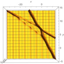
5 Solitons on elliptic backgrounds

As remarked in remark 3.3 if all tit_{i}, pjp_{j} are real, τ0(t)>0\tau_{0}(t)>0 for any tt[6], BI0B_{I}\geq 0 for any II and p11<<pL1p_{1}^{-1}<\cdots<p_{L}^{-1}, then τ(t)\tau(t) given by (3.12) is positive. Notice that τ(t)\tau(t) is a linear combination of {eηIτ0(t[pI])}\{e^{\eta_{I}}\tau_{0}(t-[p_{I}])\}. Then, in the region of the xyxy-plane such that eηIτ0(t[pI])e^{\eta_{I}}\tau_{0}(t-[p_{I}]) is dominant, u(t)=2x2logτ(t)2x2logτ0(t)u(t)=2\partial_{x}^{2}\log\tau(t)\approx 2\partial_{x}^{2}\log\tau_{0}(t) is the quasi-periodic wave corresponding to the shift of τ0(t)\tau_{0}(t). On the boundary of two such domains, soliton like waves will appear as in the case of soliton solutions[16, 17]. Thus it is expected that u(t)u(t) represents a soliton on a quasi-periodic background. In this section we verify it by a comupter simulation in the case of genus one .

Let a,ba,b be positive real numbers. Set 2ω1=ib2\omega_{1}=-ib, 2ω2=ab2\omega_{2}=ab, Ω=ω2/ω1=ia\Omega=\omega_{2}/\omega_{1}=ia and 𝕃=2ω1+2ω1{\mathbb{L}}=2\omega_{1}{\mathbb{Z}}+2\omega_{1}{\mathbb{Z}}. Define

g2=60ω𝕃,ω01ω4,g3=140ω𝕃,ω01ω6.\displaystyle g_{2}=60\,{\sum}_{\omega\in{\mathbb{L}},\omega\neq 0}\,\frac{1}{\omega^{4}},\qquad g_{3}=140\,{\sum}_{\omega\in{\mathbb{L}},\omega\neq 0}\,\frac{1}{\omega^{6}}.

Then g2g_{2}, g3g_{3} are real. Consider the algebraic curve CC defined by the corresponding Weierstrass cubic

y2=4x3g2xg3.\displaystyle y^{2}=4x^{3}-g_{2}x-g_{3}.

Let (u)\wp(u) be the Weierstrass elliptic function. Then u((u),(u))u\mapsto(\wp(u),\wp^{\prime}(u)) gives an isomorphism between the complex torus /𝕃\mathbb{C}/{\mathbb{L}} and CC, where u=0u=0 corresponds to C\infty\in C. A basis of holomorphic one forms is du=dx/ydu=dx/y. A canonical homology basis can be taken such that

α𝑑u=2ω1,β𝑑u=2ω2.\displaystyle\int_{\alpha}du=2\omega_{1},\hskip 14.22636pt\int_{\beta}du=2\omega_{2}.

Therefore the normalized holomorphic one form is given by

dv=(2ω1)1du.\displaystyle dv=(2\omega_{1})^{-1}du.

We take uu as a local coordinate around \infty. Then the corresponding solution of the KP hierarchy is given by

τ0(t)=e12q(t)θ(x2ω1+e|Ω),\displaystyle\tau_{0}(t)=e^{\frac{1}{2}q(t)}\theta\left(\frac{x}{2\omega_{1}}+e|\Omega\right),\hskip 28.45274pt (5.1)

where ee is an arbitrary complex constant. If we take eie\in i{\mathbb{R}} and xx, tjt_{j}, j2j\geq 2 to be real then τ0(t)\tau_{0}(t) is real and positive.

In the present case qi,jq_{i,j} defining q(t)q(t) is described in the following way. Let

θ11(z|Ω)=neπiΩ(n+12)2+2πi(n+12)(z+12).\displaystyle\theta_{11}(z|\Omega)=\sum_{n\in\mathbb{Z}}e^{\pi i\Omega(n+\frac{1}{2})^{2}+2\pi i(n+\frac{1}{2})(z+\frac{1}{2})}.

Sometimes θ11(z|Ω)\theta_{11}(z|\Omega) is simply denoted by θ11(z)\theta_{11}(z). It satisfies

θ11(z)=θ11(z),θ11(z)=θ11(0)z+O(z3),θ11(0)0.\displaystyle\theta_{11}(-z)=-\theta_{11}(z),\hskip 14.22636pt\theta_{11}(z)=\theta^{\prime}_{11}(0)z+O(z^{3}),\quad\theta_{11}^{\prime}(0)\neq 0.

The prime form is written as

E(z1,z2)=2ω1θ11(0)θ11(z2z12ω1).\displaystyle E(z_{1},z_{2})=\frac{2\omega_{1}}{\theta_{11}^{\prime}(0)}\theta_{11}\left(\frac{z_{2}-z_{1}}{2\omega_{1}}\right).

Therefore

2z1z2logθ11(z2z12ω1)z2z1=i,j=1qi,jz1i1z2j1.\displaystyle\frac{\partial^{2}}{\partial z_{1}\partial z_{2}}\log\frac{\theta_{11}\left(\frac{z_{2}-z_{1}}{2\omega_{1}}\right)}{z_{2}-z_{1}}=\sum_{i,j=1}^{\infty}q_{i,j}z_{1}^{i-1}z_{2}^{j-1}. (5.2)

Let us take the elliptic solution (5.1) as τ0(t)\tau_{0}(t) in the general formula (3.12).

To neatly write τ(t)\tau(t) let us introduce

F(z)=logθ11(z2ω1),Fj(z)=(1)j1(j1)!F(j)(z).\displaystyle F(z)=\log\theta_{11}\left(\frac{z}{2\omega_{1}}\right),\hskip 28.45274ptF_{j}(z)=\frac{(-1)^{j-1}}{(j-1)!}F^{(j)}(z).

By Proposition 3.4 we have

Proposition 5.1.

For τ0(t)\tau_{0}(t) given by (5.1) the τ(t)\tau(t) defined by (3.3) is written as

τ(t)\displaystyle\tau(t) =\displaystyle= cej=1cjtj+12q(t)\displaystyle ce^{\sum_{j=1}^{\infty}c_{j}t_{j}+\frac{1}{2}q(t)} (5.3)
×IBICIejIk=1tkFk(pj)θ(xjIpj2ω1+e|Ω).\displaystyle\times\sum_{I}B_{I}C_{I}e^{\sum_{j\in I}\sum_{k=1}^{\infty}t_{k}F_{k}(p_{j})}\theta\left(\frac{x-\sum_{j\in I}p_{j}}{2\omega_{1}}+e|\Omega\right).

Here cc, cjc_{j} are certain constants and

CI=jIpjθ11(pj2ω1)Nj,kI,j<kθ11(pkpj2ω1).\displaystyle C_{I}=\prod_{j\in I}\frac{p_{j}}{\theta_{11}\left(\frac{p_{j}}{2\omega_{1}}\right)^{N}}\prod_{j,k\in I,j<k}\theta_{11}\left(\frac{p_{k}-p_{j}}{2\omega_{1}}\right).

We take {tj}\{t_{j}\}, {pj}\{p_{j}\} are real and eie\in i{\mathbb{R}}. If BICI0B_{I}C_{I}\geq 0 for any II and some of them is positive then the I\sum_{I} part in the right hand side of (5.3) is positive and u=2x2logτ(t)u=2\partial^{2}_{x}\log\tau(t) is non-singular.

For the positivity of CIC_{I} we have

Proposition 5.2.

If p1<<pLp_{1}<\cdots<p_{L}, pLp1<abp_{L}-p_{1}<ab and |pj|<ab|p_{j}|<ab for 1jL1\leq j\leq L then CI>0C_{I}>0 for any II.

This proposition follows from the following lemma which can easily be proved.

Lemma 5.3.

If a>0a>0, then iθ11(ix|ia)>0i\theta_{11}(ix|ia)>0 for 0<x<a0<x<a.


Example 5.4.

Take M=N=2M=N=2, a=1a=1, b=6b=6, (p1,p2,p3,p4)=(0.31,0.46,0.81,4.89)(p_{1},p_{2},p_{3},p_{4})=(0.31,0.46,0.81,4.89), tj=0t_{j}=0 for j4j\geq 4 and

B=(10012130).\displaystyle B=\left(\begin{array}[]{cc}1&0\\ 0&1\\ -2&1\\ -3&0\\ \end{array}\right). (5.8)

This BB corresponds to (3) of §4.6.4 [17]. Notice that the matrix in [17] is the transpose of our matrix BB. In this case B12=1B_{12}=1, B13=1B_{13}=1, B14=0B_{14}=0, B23=2B_{23}=2, B24=3B_{24}=3, B34=3B_{34}=3 and

(F(1)(p1),F(1)(p2),F(1)(p3),F(1)(p4))=(3.25,2.21,1.30,0.05).\displaystyle(F^{(1)}(p_{1}),F^{(1)}(p_{2}),F^{(1)}(p_{3}),F^{(1)}(p_{4}))=(3.25,2.21,1.30,0.05). (5.9)

The results of a computer simulation of u(t)u(t) is given in figures 1,2,3. We can see the soliton corresponding to the matrix BB on the periodic waves.


Example 5.5.

Take M,N,a,b,pj,tjM,N,a,b,p_{j},t_{j} the same as those in Example 5.4. Consider BB of the form

B=(10011211).\displaystyle B=\left(\begin{array}[]{cc}1&0\\ 0&1\\ -1&2\\ -1&1\\ \end{array}\right). (5.14)

For this matrix B12=1B_{12}=1, B13=2B_{13}=2, B14=1B_{14}=1, B23=1B_{23}=1, B24=1B_{24}=1, B34=1B_{34}=1. This BB corresponds to (1) of §4.6.4 [17]. See figures 4,5,6.

Refer to caption
(a) from above
Refer to caption
(b) from an agngle
Figure 1: Example 5.4 t=3t=-3, 20x20-20\leq x\leq 20, 0y150\leq y\leq 15
Refer to caption
(a) from above
Refer to caption
(b) from an agngle
Figure 2: Example 5.4 t=0t=0, 20x20-20\leq x\leq 20, 10y10-10\leq y\leq 10
Refer to caption
(a) from above
Refer to caption
(b) from an agngle
Figure 3: Example 5.4 t=3t=3, 20x35-20\leq x\leq 35, 25y5-25\leq y\leq-5
Refer to caption
(a) from above
Refer to caption
(b) from an agngle
Figure 4: Example 5.5 t=2t=-2, 35x15-35\leq x\leq 15, 5y15-5\leq y\leq 15
Refer to caption
(a) from above
Refer to caption
(b) from an agngle
Figure 5: Example 5.5 t=0t=0, 20x20-20\leq x\leq 20, 10y10-10\leq y\leq 10
Refer to caption
(a) from above
Refer to caption
(b) from an agngle
Figure 6: Example 5.5 t=2t=2, 20x32-20\leq x\leq 32, 25y0-25\leq y\leq 0

6 Proof of Theorem 3.7 (i)

In this section we freely use notation on sheaf cohomologies. Namely, for a holomorphic line bundle {\cal L}, distinct points SiS_{i}, 1im1\leq i\leq m, SjS_{j}^{\prime}, 1jm1\leq j\leq m^{\prime} on CC, PP and positive integers {mi}\{m_{i}\}, {mj}\{m_{j}^{\prime}\} we denote

H0(C,(miSi+mjSj+P))\displaystyle H^{0}(C,{\cal L}(-\sum m_{i}S_{i}+\sum m^{\prime}_{j}S_{j}^{\prime}+\ast P))

the space of meromorphic sections of {\cal L} which have a zero at SiS_{i} of order at least mim_{i}, a pole at SjS_{j} of order at most mjm_{j}^{\prime} and a pole at PP of any order.

To prove Theorem 3.7 (i) it is sufficient to show

dimWe(n)=nN for n>>0,\displaystyle\dim W_{e}(n)=n-N\text{ for $n>>0$}, (6.1)

by Corollary 2.2.

Lemma 6.1.

There exists FiF_{i} in H0(C,LΔ,e(p))H^{0}(C,L_{\Delta,e}(\ast p_{\infty})), 1iL1\leq i\leq L such that

Fi(pj)=δi,j.\displaystyle F_{i}(p_{j})=\delta_{i,j}.

The proof of this lemma is given in the end of this section.

For 1mM1\leq m\leq M set

φm=FN+mi=1NbN+m,iFi.\displaystyle\varphi_{m}=F_{N+m}-\sum_{i=1}^{N}b^{\prime}_{N+m,i}F_{i}. (6.2)

Then

φmWe,\displaystyle\varphi_{m}\in W_{e},

since

φm(ql)=δm,l,φm(pi)=bN+m,i,\displaystyle\varphi_{m}(q_{l})=\delta_{m,l},\hskip 28.45274pt\varphi_{m}(p_{i})=-b^{\prime}_{N+m,i}, (6.3)

and

j=1MbN+j,iφm(qj)=bN+m,i=φm(pi).\displaystyle-\sum_{j=1}^{M}b^{\prime}_{N+j,i}\,\varphi_{m}(q_{j})=-b^{\prime}_{N+m,i}=\varphi_{m}(p_{i}).

Notice that the vector space

H0(C,LΔ,e(j=1LPj+p))\displaystyle H^{0}(C,L_{\Delta,e}(-\sum_{j=1}^{L}P_{j}+\ast p_{\infty}))

is a subspace of WeW_{e}, since elements of it vanish at all pjp_{j} and the linear equations imposed in WeW_{e} are trivially satisfied.

Lemma 6.2.

The following equation holds,

We=H0(C,LΔ,e(j=1LPj+p))m=1Mφm.\displaystyle W_{e}=H^{0}(C,L_{\Delta,e}(-\sum_{j=1}^{L}P_{j}+\ast p_{\infty}))\oplus\oplus_{m=1}^{M}{\mathbb{C}}\varphi_{m}. (6.4)

Proof. It is obvious that the right hand side is included in the left hand side. Let us prove the converse inclusion.

Take any fWef\in W_{e} and set f(qi)=cif(q_{i})=c_{i}. Set

F=fm=1Mcmφm.\displaystyle F=f-\sum_{m=1}^{M}c_{m}\varphi_{m}.

Then

F(qi)=f(qi)m=1Mcmφm(qi)=cici=0.\displaystyle F(q_{i})=f(q_{i})-\sum_{m=1}^{M}c_{m}\varphi_{m}(q_{i})=c_{i}-c_{i}=0.

Since ff and φl\varphi_{l} are both in WeW_{e}, FWeF\in W_{e} and F(pi)=0F(p_{i})=0 for 1iN1\leq i\leq N. Therefore

FH0(C,LΔ,e(j=1LPj+p))\displaystyle F\in H^{0}(C,L_{\Delta,e}(-\sum_{j=1}^{L}P_{j}+\ast p_{\infty}))

and therefore ff is in the right hand side of (6.4). ∎

Take nn larger than the order of a pole of φj\varphi_{j} at pp_{\infty} for any jj. Then

We(n)=H0(C,LΔ,e(j=1LPj+np))m=1Mφm,\displaystyle W_{e}(n)=H^{0}(C,L_{\Delta,e}(-\sum_{j=1}^{L}P_{j}+np_{\infty}))\oplus\oplus_{m=1}^{M}{\mathbb{C}}\varphi_{m},

and

dimWe(n)=dimH0(C,LΔ,e(j=1LPj+np))+M.\displaystyle\dim W_{e}(n)=\dim H^{0}(C,L_{\Delta,e}(-\sum_{j=1}^{L}P_{j}+np_{\infty}))+M.

If we further take nn larger than g1+Lg-1+L,

degLΔ,e(j=1LPj+np)=g1L+n>2g2=degΩ1,\displaystyle\deg L_{\Delta,e}(-\sum_{j=1}^{L}P_{j}+np_{\infty})=g-1-L+n>2g-2=\deg\Omega^{1},

then

H1(C,LΔ,e(j=1LPj+np))=0,\displaystyle H^{1}(C,L_{\Delta,e}(-\sum_{j=1}^{L}P_{j}+np_{\infty}))=0,

and, by the Riemann-Roch theorem,

dimH0(C,LΔ,e(j=1LPj+np))=nL.\displaystyle\dim H^{0}(C,L_{\Delta,e}(-\sum_{j=1}^{L}P_{j}+np_{\infty}))=n-L.

Therefore, for n>>0n>>0,

dimWe(n)=nL+M=nN.\displaystyle\dim W_{e}(n)=n-L+M=n-N.

Proof of Lemma 6.1.

We first show that, for each 1iL1\leq i\leq L, there exists an element GiG_{i} of H0(C,LΔ,e(p))H^{0}(C,L_{\Delta,e}(\ast p_{\infty})) such that it has only a simple pole at PiP_{i} on C\{p}C\backslash\{p_{\infty}\}.

By the Riemann-Roch theorem, for a sufficiently large nn, we have

dimH0(C,LΔ,e(Pi+np))=n+1,\displaystyle\dim H^{0}(C,L_{\Delta,e}(P_{i}+np_{\infty}))=n+1,
dimH0(C,LΔ,e(np))=n.\displaystyle\dim H^{0}(C,L_{\Delta,e}(np_{\infty}))=n.

It means that there exists a meromorphic section of LΔ,eL_{\Delta,e} which has a simple pole at PiP_{i}, a pole at pp_{\infty} of order at most nn and has no other poles. Thus GiG_{i} exists.

Next we prove that there exists a meromorphic function on CC such that it has a simple zero at every PiP_{i}, 1iL1\leq i\leq L, and it is holomorphic on C\{p}C\backslash\{p_{\infty}\}.

Again, if we take nn sufficiently large, we have, by the Riemann-Roch theorem,

dimH0(C,𝒪(j=1LPj+np))=1gL+n,\displaystyle\dim H^{0}(C,{\cal O}(-\sum_{j=1}^{L}P_{j}+np_{\infty}))=1-g-L+n,
dimH0(C,𝒪(Pij=1LPj+np))=gL+n.\displaystyle\dim H^{0}(C,{\cal O}(-P_{i}-\sum_{j=1}^{L}P_{j}+np_{\infty}))=-g-L+n.

It follows that, for each iLi\leq L, there exists a meromorphic function hih_{i} on CC which has a simple zero at PiP_{i}, a zero at PjP_{j}, jij\neq i, and is holomorphic on C\{p}C\backslash\{p_{\infty}\}. We shall show that a desired hh can be constructed as a linear combination of {hi}\{h_{i}\}.

Set

h=i=1Lλihi.\displaystyle h=\sum_{i=1}^{L}\lambda_{i}h_{i}.

At each PiP_{i} take a local coordinate ww and write

hi=ciw+O(w2),hj=cjwmj+O(wmj+1),ji,\displaystyle h_{i}=c_{i}w+O(w^{2}),\hskip 28.45274pth_{j}=c_{j}w^{m_{j}}+O(w^{m_{j}+1}),\quad j\neq i,

where cj0c_{j}\neq 0 for any jj. Let {j|mj=1}={j1,,jr}\{j\,|\,m_{j}=1\}=\{j_{1},...,j_{r}\}, where we set mi=1m_{i}=1. Then

h=(cj1λj1++cjrλjr)w+O(w2),\displaystyle h=(c_{j_{1}}\lambda_{j_{1}}+\cdots+c_{j_{r}}\lambda_{j_{r}})w+O(w^{2}),

and the condition that hh has a simple zero at PiP_{i} is

cj1λj1++cjrλjr0.\displaystyle c_{j_{1}}\lambda_{j_{1}}+\cdots+c_{j_{r}}\lambda_{j_{r}}\neq 0. (6.5)

This is an open condition for {λj}\{\lambda_{j}\}. Thus there exists {λj}\{\lambda_{j}\} such that hh has a simple zero at every PiP_{i}.

Choosing one set of {h,Gi|1iL}\{h,G_{i}|1\leq i\leq L\} define the element of H0(C,LΔ,e(p))H^{0}(C,L_{\Delta,e}(\ast p_{\infty})) by

Fi=aihGi,ai=(hGi)(pi)1.\displaystyle F_{i}=a_{i}hG_{i},\quad a_{i}=(hG_{i})(p_{i})^{-1}.

Obviously they satisfy Fi(pj)=δi,jF_{i}(p_{j})=\delta_{i,j}. ∎

7 Proof of Theorem 3.7 (ii)

Let Ψ(t,z)\Psi(t,z) be the wave function of τ(t)\tau(t),

Ψ(t,z)=τ(t[z])τ(t)eη(t,z1).\displaystyle\Psi(t,z)=\frac{\tau(t-[z])}{\tau(t)}e^{\eta(t,z^{-1})}. (7.1)

We first show

Lemma 7.1.

For 1iN1\leq i\leq N

Ψ(t,pi)=j=1Mb~N+j,iΨ(t,pN+j),b~N+j,i=bN+j,i(pipN+j1)N\displaystyle\Psi(t,p_{i})=-\sum_{j=1}^{M}\tilde{b}_{N+j,i}\Psi(t,p_{N+j}),\quad\tilde{b}_{N+j,i}=b_{N+j,i}(p_{i}p_{N+j}^{-1})^{N} (7.2)

Proof. Substitute (7.1) into (7.2) we have the equation for τ(t)\tau(t),

τ(t[pi])eηi=j=1Mb~N+j,iτ(t[pN+j])eηN+j.\displaystyle\tau(t-[p_{i}])e^{\eta_{i}}=-\sum_{j=1}^{M}\tilde{b}_{N+j,i}\tau(t-[p_{N+j}])e^{\eta_{N+j}}. (7.3)

Let us prove this equation.

By (3.12) we have, using eη([z],p1)=1p1ze^{-\eta([z],p^{-1})}=1-p^{-1}z,

τ(t[z])=IBIΔIjI(1pj1z)eηIτ0(t[z][pI]).\displaystyle\tau(t-[z])=\sum_{I}B_{I}\Delta^{-}_{I}\prod_{j\in I}(1-p_{j}^{-1}z)\,e^{\eta_{I}}\tau_{0}(t-[z]-[p_{I}]). (7.4)

Substituting z=piz=p_{i}, 1iN1\leq i\leq N and multiplying by eηie^{\eta_{i}} we get

τ(t[pi])eηi\displaystyle\tau(t-[p_{i}])e^{\eta_{i}} =\displaystyle= piNIBIΔIjI(pi1pj1)eηI+ηiτ0(t[pi][pI])\displaystyle p_{i}^{N}\sum_{I}B_{I}\Delta_{I}^{-}\prod_{j\in I}(p_{i}^{-1}-p_{j}^{-1})e^{{\eta_{I}}+\eta_{i}}\tau_{0}(t-[p_{i}]-[p_{I}]) (7.5)
=\displaystyle= piNiIBIΔ(I,i)eη(I,i)τ0(t[p(I,i)]).\displaystyle p_{i}^{N}\sum_{i\notin I}B_{I}\Delta_{(I,i)}^{-}e^{\eta_{(I,i)}}\tau_{0}(t-[p_{(I,i)}]).

We write I=(I,N+j1,,N+jr)I=(I^{\prime},N+j_{1},...,N+j_{r}) with

I([N]Nr),1j1<<jrM.\displaystyle I^{\prime}\in\binom{[N]}{N-r},\quad 1\leq j_{1}<\cdots<j_{r}\leq M.

Since iIi\notin I, we have r1r\geq 1 and iIi\notin I^{\prime}. For simplicity we set

T(I,i)=eη(I,i)τ0(t[p(I,i)]).\displaystyle T(I,i)=e^{\eta_{(I,i)}}\tau_{0}(t-[p_{(I,i)}]). (7.6)

Then

RHS of (7.5) (7.7)
=\displaystyle= piNr=1NI([N]Nr),iI,1j1<<jrMB(I,N+j1,,N+jr)Δ(I,N+j1,,N+jr,i)\displaystyle p_{i}^{N}\sum_{r=1}^{N}\sum_{I^{\prime}\in\binom{[N]}{N-r},i\notin I^{\prime},1\leq j_{1}<\cdots<j_{r}\leq M}B_{(I^{\prime},N+j_{1},...,N+j_{r})}\Delta^{-}_{(I^{\prime},N+j_{1},...,N+j_{r},i)}
×T(I,N+j1,,N+jr,i).\displaystyle\times T(I^{\prime},N+j_{1},...,N+j_{r},i).

To proceed we extend the index II of BIB_{I} and ΔI\Delta^{-}_{I} to arbitrary sequence from [L][L] in a skew symmetric way. In particular, for I=(i1,,iN)I=(i_{1},...,i_{N}), BIΔIB_{I}\Delta^{-}_{I} is symmetric in i1,,iNi_{1},...,i_{N} and BIB_{I}, ΔI\Delta^{-}_{I} become 0 if some of indices in II coincide.

Then

1j1<<jrMB(I,N+j1,,N+jr)Δ(I,N+j1,,N+jr,i)T(I,N+j1,,N+jr,i)\displaystyle\sum_{1\leq j_{1}<\cdots<j_{r}\leq M}B_{(I^{\prime},N+j_{1},...,N+j_{r})}\Delta^{-}_{(I^{\prime},N+j_{1},...,N+j_{r},i)}T(I^{\prime},N+j_{1},...,N+j_{r},i) (7.8)
=\displaystyle= 1r!j1,,jr=1MB(I,N+j1,,N+jr)Δ(I,N+j1,,N+jr,i)T(I,N+j1,,N+jr,i).\displaystyle\frac{1}{r!}\sum_{j_{1},...,j_{r}=1}^{M}B_{(I^{\prime},N+j_{1},...,N+j_{r})}\Delta^{-}_{(I^{\prime},N+j_{1},...,N+j_{r},i)}T(I^{\prime},N+j_{1},...,N+j_{r},i).

Recall that BB has the form

B=(11bN+1,1bN+1,NbN+M,1bN+M,N).\displaystyle B=\left(\begin{array}[]{ccc}1&&\\ &\ddots&\\ &&1\\ b_{N+1,1}&\cdots&b_{N+1,N}\\ \vdots&&\vdots\\ b_{N+M,1}&\cdots&b_{N+M,N}\\ \end{array}\right). (7.15)

and iIi\notin I^{\prime}. Then the expansion of the determinant B(I,N+j1,,N+jr)B_{(I^{\prime},N+j_{1},...,N+j_{r})} in the ii-th column takes the form

B(I,N+j1,,N+jr)=k=1r(1)Nr+k+ibN+jk,iB(I,N+j1,,N+jk^,,N+jr)(i).\displaystyle B_{(I^{\prime},N+j_{1},...,N+j_{r})}=\sum_{k=1}^{r}(-1)^{N-r+k+i}b_{N+j_{k},i}B^{(i)}_{(I^{\prime},N+j_{1},...,\widehat{N+j_{k}},...,N+j_{r})}. (7.16)

Here Bi1,,iN1(i)B^{(i)}_{i_{1},...,i_{N-1}} denotes the determinant det(bim,j)1mN1,1jN,ji\det(b_{i_{m},j})_{1\leq m\leq N-1,1\leq j\leq N,j\neq i}. Substitute (7.16) into (7.8) and change the order of sum:

RHS of (7.8) (7.17)
=\displaystyle= 1r!k=1rj1,,jr=1M(1)Nr+k+ibN+jk,iB(I,N+j1,,N+jk^,,N+jr)(i)Δ(I,N+j1,,N+jr,i)\displaystyle\frac{1}{r!}\sum_{k=1}^{r}\sum_{j_{1},...,j_{r}=1}^{M}(-1)^{N-r+k+i}b_{N+j_{k},i}B^{(i)}_{(I^{\prime},N+j_{1},...,\widehat{N+j_{k}},...,N+j_{r})}\Delta^{-}_{(I^{\prime},N+j_{1},...,N+j_{r},i)}
×T(I,N+j1,,N+jr,i).\displaystyle\times T(I^{\prime},N+j_{1},...,N+j_{r},i).

Use

Δ(I,N+j1,,N+jr,i)=(1)rkΔ(I,N+j1,,N+jk^,,N+jr,N+jk,i)\displaystyle\Delta^{-}_{(I^{\prime},N+j_{1},...,N+j_{r},i)}=(-1)^{r-k}\Delta^{-}_{(I^{\prime},N+j_{1},...,\widehat{N+j_{k}},...,N+j_{r},N+j_{k},i)}

and change the names of indices as jkjj_{k}\rightarrow j, j1,,jk^,,jrj_{1},...,\widehat{j_{k}},...,j_{r} \rightarrow j1,,jr1j_{1},...,j_{r-1}. We get

RHS of (7.17)
=\displaystyle= 1r!k=1r(1)N+ij=1MbN+j,ij1,,jr1=1MB(I,N+j1,,N+jr1)(i)Δ(I,N+j1,,N+jr1,N+j,i)\displaystyle\frac{1}{r!}\sum_{k=1}^{r}(-1)^{N+i}\sum_{j=1}^{M}b_{N+j,i}\sum_{j_{1},...,j_{r-1}=1}^{M}B^{(i)}_{(I^{\prime},N+j_{1},...,N+j_{r-1})}\Delta^{-}_{(I^{\prime},N+j_{1},...,N+j_{r-1},N+j,i)}
×T(I,N+j1,,N+jr1,N+j,i).\displaystyle\times T_{(I^{\prime},N+j_{1},...,N+j_{r-1},N+j,i)}.

Since the summand does not depend on kk, the sum in kk gives rr times of the summand. Rewrite the summation in 1j1,,jr1M1\leq j_{1},...,j_{r-1}\leq M to (r1)!(r-1)! times the summation in (j1,,jr1)(j_{1},...,j_{r-1}) with 1<j1<<jr1M1<j_{1}<\cdots<j_{r-1}\leq M. Subsitute it into (7.7) and get

RHS of (7.7)
=\displaystyle= (1)N+ipiNj=1NbN+j,ir=1MI([N]Nr),iI1j1<<jr1MB(I,N+j1,,N+jr1)(i)\displaystyle(-1)^{N+i}p_{i}^{N}\sum_{j=1}^{N}b_{N+j,i}\sum_{r=1}^{M}\sum_{I^{\prime}\in\binom{[N]}{N-r},i\notin I^{\prime}}\sum_{1\leq j_{1}<\cdots<j_{r-1}\leq M}B^{(i)}_{(I^{\prime},N+j_{1},...,N+j_{r-1})}
×Δ(I,N+j1,,N+jr1,N+j,i)T(I,N+j1,,N+jr1,N+j,i).\displaystyle\times\Delta^{-}_{(I^{\prime},N+j_{1},...,N+j_{r-1},N+j,i)}T_{(I^{\prime},N+j_{1},...,N+j_{r-1},N+j,i)}.

Notice that taking the summation over rr, II^{\prime}, {jk}\{j_{k}\} is equivalent to taking the summation over I([L]N1)I^{\prime}\in\binom{[L]}{N-1} with i,N+jIi,N+j\notin I^{\prime}. Thus

τ(t[pi])eηi\displaystyle\tau(t-[p_{i}])e^{\eta_{i}} (7.18)
=\displaystyle= RHS of (7.7)
=\displaystyle= (1)N+ipiNj=1NbN+j,iI([L]N1),i,N+jIBI(i)Δ(I,N+j,i)T(I,N+j,i).\displaystyle(-1)^{N+i}p_{i}^{N}\sum_{j=1}^{N}b_{N+j,i}\sum_{I^{\prime}\in\binom{[L]}{N-1},i,N+j\notin I^{\prime}}B^{(i)}_{I^{\prime}}\Delta^{-}_{(I^{\prime},N+j,i)}T(I^{\prime},N+j,i).

Next, by replacing ii by N+jN+j in (7.5) and recalling the definition (7.6) of T(I,i)T(I,i), we have

τ(t[pN+j])eηN+j=pN+jNN+jIBIΔ(I,N+j)T(I,N+j).\displaystyle\tau(t-[p_{N+j}])e^{\eta_{N+j}}=p_{N+j}^{N}\sum_{N+j\notin I}B_{I}\Delta_{(I,N+j)}^{-}T(I,N+j). (7.19)

It follows that

j=1Mb~N+j,iτ(t[pN+j])eηN+j\displaystyle\sum_{j=1}^{M}\tilde{b}_{N+j,i}\tau(t-[p_{N+j}])e^{\eta_{N+j}} (7.20)
=\displaystyle= piNj=1MbN+j,iN+jIBIΔ(I,N+j)T(I,N+j)\displaystyle p_{i}^{N}\sum_{j=1}^{M}b_{N+j,i}\sum_{N+j\notin I}B_{I}\Delta_{(I,N+j)}^{-}T(I,N+j)
=\displaystyle= I++I,\displaystyle I_{+}+I_{-}, (7.21)

where I+I_{+} is the part of the RHS of (7.20) such that II includes ii in the summation over II and II_{-} the part where II does not include ii.

We show that I+I_{+} is equal to τ(t[pi])eηi-\tau(t-[p_{i}])e^{\eta_{i}} and I=0I_{-}=0.

Let us first consider I+I_{+}. Separating ii from II we have

I+=piNj=1MbN+j,iI([L]N1),i,N+jIB(I,i)Δ(I,i,N+j)T(I,i,N+j).\displaystyle I_{+}=p_{i}^{N}\sum_{j=1}^{M}b_{N+j,i}\sum_{I^{\prime}\in\binom{[L]}{N-1},i,N+j\notin I}B_{(I^{\prime},i)}\Delta_{(I^{\prime},i,N+j)}^{-}T(I^{\prime},i,N+j).

Since the NN-th row vector of B(I,i)B_{(I^{\prime},i)} is the ii-th unit vector, we have

B(I,i)=(1)N+iBI(i).\displaystyle B_{(I^{\prime},i)}=(-1)^{N+i}B_{I^{\prime}}^{(i)}.

Therefore

I+\displaystyle I_{+} =\displaystyle= (1)N+ipiNj=1MbN+j,iI([L]N1),i,N+jIBI(i)Δ(I,i,N+j)T(I,i,N+j)\displaystyle(-1)^{N+i}p_{i}^{N}\sum_{j=1}^{M}b_{N+j,i}\sum_{I^{\prime}\in\binom{[L]}{N-1},i,N+j\notin I}B_{I^{\prime}}^{(i)}\Delta_{(I^{\prime},i,N+j)}^{-}T(I^{\prime},i,N+j) (7.22)
=\displaystyle= RHS of (7.18)\displaystyle-\text{RHS of (\ref{tau-pi-5})}
=\displaystyle= τ(t[pi])eηi,\displaystyle-\tau(t-[p_{i}])e^{\eta_{i}},

where Δ(I,i,N+j)=Δ(I,N+j,i)\Delta_{(I^{\prime},i,N+j)}^{-}=-\Delta_{(I^{\prime},N+j,i)}^{-} is used.

Next let us consider II_{-}. In a similar computation to deriving (7.18) we have

I\displaystyle I_{-} =\displaystyle= (1)N+ij=1MbN+j,ij=1MbN+j,iI([L]N1),i,N+j,N+jIBI(i)Δ(I,N+j,N+j)\displaystyle(-1)^{N+i}\sum_{j=1}^{M}b_{N+j,i}\sum_{j^{\prime}=1}^{M}b_{N+j^{\prime},i}\sum_{I^{\prime}\in\binom{[L]}{N-1},i,N+j^{\prime},N+j\notin I^{\prime}}B^{(i)}_{I^{\prime}}\Delta^{-}_{(I^{\prime},N+j^{\prime},N+j)}
×T(I,N+j,N+j)\displaystyle\times T(I^{\prime},N+j^{\prime},N+j)
=\displaystyle= (1)N+ij,j=1MbN+j,ibN+j,iI([L]N1),i,N+j,N+jIBI(i)Δ(I,N+j,N+j)\displaystyle(-1)^{N+i}\sum_{j,j^{\prime}=1}^{M}b_{N+j,i}b_{N+j^{\prime},i}\sum_{I^{\prime}\in\binom{[L]}{N-1},i,N+j^{\prime},N+j\notin I^{\prime}}B^{(i)}_{I^{\prime}}\Delta^{-}_{(I^{\prime},N+j^{\prime},N+j)}
×T(I,N+j,N+j).\displaystyle\times T(I^{\prime},N+j^{\prime},N+j).

Since bN+j,ibN+j,ib_{N+j,i}b_{N+j^{\prime},i} is symmetric in j,jj,j^{\prime} and the remaining part is skew symmetric in j,jj,j^{\prime}, the last summation in j,jj,j^{\prime} becomes zero. Therefore I=0I_{-}=0. We, then, have (7.3) by (7.21), (7.22). ∎

By Lemma 3.5 we have

Lemma 7.2.

Let N1N\geq 1, QjCQ_{j}\in C, 1jN1\leq j\leq N and zj=z(Qj)z_{j}=z(Q_{j}). Then

τ0(t[z]j=1N[zj])eη(t,z1)\displaystyle\tau_{0}(t-[z]-\sum_{j=1}^{N}[z_{j}])e^{\eta(t,z^{-1})} (7.23)
=\displaystyle= (zE(0,z))N+1j=1NE(z,zj)zjzj=1NzjE(0,zj)eq(j=1N[zj])j=1NQ(t|[zj])+12q(t)\displaystyle\left(\frac{z}{E(0,z)}\right)^{N+1}\prod_{j=1}^{N}\frac{E(z,z_{j})}{z_{j}-z}\prod_{j=1}^{N}\frac{z_{j}}{E(0,z_{j})}e^{q(\sum_{j=1}^{N}[z_{j}])-\sum_{j=1}^{N}Q(t|[z_{j}])+\frac{1}{2}q(t)}
×θ(𝒱tI(p)j=1NI(Qj)+e)ej=1tjp𝑑r~j.\displaystyle\times\theta({\cal V}t-I(p)-\sum_{j=1}^{N}I(Q_{j})+e)e^{\sum_{j=1}^{\infty}t_{j}\int^{p}d\tilde{r}_{j}}.

We use (7.23) to compute (7.4) and get

τ(t[z])eη(t,z1)\displaystyle\tau(t-[z])e^{\eta(t,z^{-1})} (7.24)
=\displaystyle= zN+1J([L]N)BJΔJeηJjJE(z,pj)E(0,z)E(0,pj)eq(jJ[pj])jJQ(t|[pj])+12q(t)\displaystyle z^{N+1}\sum_{J\in\binom{[L]}{N}}B_{J}\Delta^{-}_{J}e^{\eta_{J}}\prod_{j\in J}\frac{E(z,p_{j})}{E(0,z)E(0,p_{j})}e^{q(\sum_{j\in J}[p_{j}])-\sum_{j\in J}Q(t|[p_{j}])+\frac{1}{2}q(t)}
×1E(0,z)θ(𝒱tI(p)jJI(Qj)+e)ej=1tjp𝑑r~j.\displaystyle\times\frac{1}{E(0,z)}\theta({\cal V}t-I(p)-\sum_{j\in J}I(Q_{j})+e)e^{\sum_{j=1}^{\infty}t_{j}\int^{p}d\tilde{r}_{j}}.

Set

Ψ(t,z)=zN1Ψ(t,z).\displaystyle\Psi^{\prime}(t,z)=z^{-N-1}\Psi(t,z).

Then (7.24) shows that the expansion coefficients of τ(t)Ψ(t,z)=zN1τ(t[z])eη(t,z1)\tau(t)\Psi^{\prime}(t,z)=z^{-N-1}\tau(t-[z])e^{\eta(t,z^{-1})} belong to H0(C,LΔ,e(p))H^{0}(C,L_{\Delta,e}(\ast p_{\infty})). Rewriting the equation (7.2) in terms of Ψ(t,z)\Psi^{\prime}(t,z) we have

Ψ(t,pi)=j=1MbN+j,iΨ(t,qj).\displaystyle\Psi^{\prime}(t,p_{i})=-\sum_{j=1}^{M}b^{\prime}_{N+j,i}\Psi^{\prime}(t,q_{j}).

It means that the expansion coefficients of τ(t)Ψ(t,z)\tau(t)\Psi^{\prime}(t,z) are in WeW_{e}. Thus the expansion coefficients of τ(t)Ψ(t,z)\tau(t)\Psi(t,z) are in zN+1We=Uez^{N+1}W_{e}=U_{e}. Since UeUGMU_{e}\in UGM by (1) of Theorem 3.7 and the strict inclusion relation is impossible for points of UGM, UeU_{e} is the point of UGM corresponding to τ(t)\tau(-t). ∎

Appendix A Proof of Proposition 4.1

We first show that ReR_{e} is contained in the RHS of (4.1). Let fRef\in R_{e} and φmWe\varphi_{m}\in W_{e} be defined in (6.2). Then fφmWef\varphi_{m}\in W_{e}. By (6.3) we see that

(fφm)(pi)=j=1MbN+j,i(fφm)(qj)\displaystyle(f\varphi_{m})(p_{i})=-\sum_{j=1}^{M}b^{\prime}_{N+j,i}(f\varphi_{m})(q_{j})

is equivalent to

f(pi)bN+m,i=bN+m,if(qm).\displaystyle f(p_{i})b^{\prime}_{N+m,i}=b^{\prime}_{N+m,i}f(q_{m}). (A.1)

Therefore ff is contained in the RHS of (4.1).

Let us prove the converse inclusion. Let ff be an element of the RHS of (4.1) and FWeF\in W_{e}. Notice that the equation (A.1) holds for any i,mi,m. Then

j=1MbN+j,i(fF)(qj)\displaystyle-\sum_{j=1}^{M}b^{\prime}_{N+j,i}(fF)(q_{j}) =\displaystyle= j=1MbN+j,if(qj)F(qj)\displaystyle-\sum_{j=1}^{M}b^{\prime}_{N+j,i}f(q_{j})F(q_{j})
=\displaystyle= j=1MbN+j,if(pi)F(qj)\displaystyle-\sum_{j=1}^{M}b^{\prime}_{N+j,i}f(p_{i})F(q_{j})
=\displaystyle= f(pi)(j=1MbN+j,iF(qj))\displaystyle f(p_{i})\left(-\sum_{j=1}^{M}b^{\prime}_{N+j,i}F(q_{j})\right)
=\displaystyle= f(pi)F(pi)=(fF)(pi)\displaystyle f(p_{i})F(p_{i})=(fF)(p_{i})

which means fFWefF\in W_{e}. Thus fRef\in R_{e}. ∎

Appendix B Proof of Theorem 4.4

(iii) follows from (ii). Let us prove (i), (ii), (iv).

(i) It can be easily proved that if φ(𝒫)=p\varphi({\cal P})=p^{\prime}_{\infty} for some 𝒫SpecRe{\cal P}\in{\rm Spec}R_{e} then 𝒫=Re{\cal P}=R_{e}. It is absurd.

(ii) Let 𝒫=n=0𝒫(n)C{\cal P}=\oplus_{n=0}^{\infty}{\cal P}^{(n)}\in C^{\prime} such that 𝒫p{\cal P}^{\prime}\neq p^{\prime}_{\infty}. Set

q=n=0𝒫(n)Re,\displaystyle q=\cup_{n=0}^{\infty}{\cal P}^{(n)}\subset Re,

which obviously becomes an ideal of ReR_{e}. It is sufficient to prove the following lemma.

Lemma B.1.

(i) If x,yRex,y\in R_{e} satisfies xyqxy\in q, either xqx\in q or yqy\in q. (ii) qReq\neq R_{e}. (iii) φ(q)=𝒫\varphi(q)={\cal P}.

Proof. (i) We can assume that

x=zm+O(zm+1),y=zn+O(zn+1)\displaystyle x=z^{-m}+O(z^{-m+1}),\hskip 28.45274pty=z^{-n}+O(z^{-n+1})

with m,n1m,n\geq 1. Then

xyRe(m+n)\Re(m+n1).\displaystyle xy\in R_{e}(m+n)\backslash R_{e}(m+n-1). (B.1)

Since xyqxy\in q, there exists N0N\geq 0 such that

xy𝒫(N)Re(N).\displaystyle xy\in{\cal P}^{(N)}\subset R_{e}(N).

By (B.1) we have Nm+nN\geq m+n. Set

N(m+n)=k0.\displaystyle N-(m+n)=k\geq 0.

Then

xRe(m)Re(m+k),yRe(n).\displaystyle x\in R_{e}(m)\subset R_{e}(m+k),\hskip 28.45274pty\in R_{e}(n).

So we consider xx and yy as homogeneous elements of AA^{\prime} with degree m+km+k and nn respectively. Then

xy𝒫(N)A.\displaystyle xy\in{\cal P}^{(N)}\subset A^{\prime}.

Since 𝒫{\cal P} is a prime ideal of AA^{\prime}, x𝒫x\in{\cal P} or y𝒫y\in{\cal P}. Therefore x𝒫Re(m+k)=𝒫(m+k)x\in{\cal P}\cap R_{e}(m+k)={\cal P}^{(m+k)} or y𝒫Re(m)=𝒫(m)y\in{\cal P}\cap R_{e}(m)={\cal P}^{(m)}. It means that xqx\in q or yqy\in q.

(ii) Notice that 1Re(n)1\in R_{e}(n) for any n0n\geq 0. If we consider 11 as a homogeneous element of AA^{\prime} with degree nn we denote it by 1(n)1^{(n)}. We shall show

1(n)𝒫(n),n0.\displaystyle 1^{(n)}\notin{\cal P}^{(n)},\hskip 28.45274ptn\geq 0. (B.2)

Since 𝒫A{\cal P}\neq A^{\prime}, 1(0)𝒫(0)1^{(0)}\notin{\cal P}^{(0)}.

Let us consider the case n=1n=1. Suppose that 1(1)𝒫(1)1^{(1)}\in{\cal P}^{(1)}. Notice that A1(1)=pA^{\prime}1^{(1)}=p^{\prime}_{\infty}. Therefore

p𝒫,\displaystyle p^{\prime}_{\infty}\subsetneq{\cal P},

since 𝒫p{\cal P}\neq p^{\prime}_{\infty}. Then there exists k1k\geq 1 and fk𝒫(k)f_{k}\in{\cal P}^{(k)} such that fkRe(k1)f_{k}\notin R_{e}(k-1), that is,

fk=zk+O(zk+1).\displaystyle f_{k}=z^{-k}+O(z^{-k+1}).

By the Riemann-Roch theorem we have

dimRe(n)/Re(n1)=1.n>>0,\displaystyle\dim R_{e}(n)/R_{e}(n-1)=1.\hskip 28.45274ptn>>0, (B.3)

It follows that, for all sufficiently large nn, there exists hnRe(n)h_{n}\in R_{e}(n) such that

hn=zn+O(zn+1).\displaystyle h_{n}=z^{-n}+O(z^{-n+1}).

Then hnfk𝒫(n+k)h_{n}f_{k}\in{\cal P}^{(n+k)} and hnfkRe(n+k)\Re(n+k1)h_{n}f_{k}\in R_{e}(n+k)\backslash R_{e}(n+k-1). Taking into account that 𝒫(n+k)Re(n+k1){\cal P}^{(n+k)}\supset R_{e}(n+k-1) we see that

𝒫(n)=Re(n),n>>0.\displaystyle{\cal P}^{(n)}=R_{e}(n),\hskip 28.45274ptn>>0. (B.4)

On the other hand

𝒫n=1Re(n)\displaystyle{\cal P}\nsupseteq\oplus_{n=1}^{\infty}R_{e}(n)

since 𝒫C{\cal P}\in C^{\prime}. It follows that there exists N1N\geq 1 and FNRe(N)F_{N}\in R_{e}(N) such that FN𝒫(N)F_{N}\notin{\cal P}^{(N)}. Since 𝒫(N)Re(N1){\cal P}^{(N)}\supset R_{e}(N-1), FNRe(N)\Re(N1)F_{N}\in R_{e}(N)\backslash R_{e}(N-1), that is,

FN=zN+O(zN+1).\displaystyle F_{N}=z^{-N}+O(z^{-N+1}).

Since 𝒫{\cal P} is a prime ideal,

FNm𝒫(Nm),\displaystyle F_{N}^{m}\notin{\cal P}^{(Nm)},

for any m1m\geq 1 which contradicts (B.4). Thus 1(1)𝒫(1)1^{(1)}\notin{\cal P}^{(1)}.

Notice that (1(1))n=1(n)(1^{(1)})^{n}=1^{(n)} for n2n\geq 2. Thus 1(n)𝒫(n)1^{(n)}\notin{\cal P}^{(n)} and (B.2) has been proved.

Then 1q1\notin q and qReq\neq R_{e}.

(iii) We have to prove that qRe(n)=𝒫(n)q\cap R_{e}(n)={\cal P}^{(n)} for any n0n\geq 0. Suppose that this does not hold. Then there exists N1N\geq 1 such that

qRe(N)𝒫(N).\displaystyle q\cap R_{e}(N)\neq{\cal P}^{(N)}.

Since the right hand side is contained in the left hand side, it means

qRe(N)𝒫(N).\displaystyle q\cap R_{e}(N)\supsetneq{\cal P}^{(N)}.

Therefore there exists xqRe(N)x\in q\cap R_{e}(N) such that x𝒫(N)x\notin{\cal P}^{(N)}. Since xqx\in q there exists MM such that x𝒫(M)x\in{\cal P}^{(M)}. Then N<MN<M. In fact if NMN\geq M, x𝒫(M)𝒫(N)x\in{\cal P}^{(M)}\subset{\cal P}^{(N)}. Since xqRe(N)x\in q\cap R_{e}(N), we can consider xx as a homogeneous element of AA^{\prime} with degree NN. Then x𝒫(N)x\notin{\cal P}^{(N)} and 1(MN)𝒫(MN)1^{(M-N)}\notin{\cal P}^{(M-N)} but

1(MN)x=x𝒫(M),\displaystyle 1^{(M-N)}x=x\in{\cal P}^{(M)},

which is absurd. Thus qRe(n)=𝒫(n)q\cap R_{e}(n)={\cal P}^{(n)} for any nn and (iii) of the lemma is proved. ∎


Proof of Theorem 4.4 (iv). It is obvious that apa\notin p^{\prime}_{\infty} and pD+(a)p^{\prime}_{\infty}\in D_{+}(a). Let

(p)(a)=n=0Re(nm1)an\displaystyle(p^{\prime}_{\infty})_{(a)}=\sum_{n=0}^{\infty}\frac{R_{e}(nm-1)}{a^{n}}

be the image of pp^{\prime}_{\infty} in A(a)A^{\prime}_{(a)}. Any element of fRe(nm)f\in R_{e}(nm) satisfies fcanRe(nm1)f-ca^{n}\in R_{e}(nm-1) for some constant cc\in{\mathbb{C}}. It means that f/an=cf/a^{n}=c modulo (p)(a)(p_{\infty})_{(a)}. Since (p)(a)A(a)(p_{\infty})_{(a)}\neq A_{(a)}, this means that A(a)/(p)(a)A_{(a)}/(p^{\prime}_{\infty})_{(a)}\simeq{\mathbb{C}}. Thus (p)(a)(p^{\prime}_{\infty})_{(a)} is a maximal ideal of A(a)A_{(a)} and (iv) is proved, ∎

Appendix C Proof of Proposition 4.5

Both WeW_{e} and ReR_{e} is a subspace of ((z)){\mathbb{C}}((z)) and the ReR_{e} module structure of WeW_{e} is given by the ring structure of ((z)){\mathbb{C}}((z)). Therefore WeW_{e} is a torsion free ReR_{e} module. That 𝒲e{\cal W}_{e} is a torsion free 𝒪C{\cal O}_{C^{\prime}} module follows from this.

Let KK^{\prime} be the quotient field of ReR_{e}. In order to prove that the rank of WeW_{e} is one, it is sufficient to show, by the definition, that dimKKReWe=1\dim_{K^{\prime}}K^{\prime}\otimes_{R_{e}}W_{e}=1.

Lemma C.1.

Let KK be the quotient field of RR. Then K=KK^{\prime}=K.

Proof. Since ReRR_{e}\subset R, KKK^{\prime}\subset K. Let us prove the converse inclusion. Take any fKf\in K. Let the pole divisor of ff be

m1R1++msRs+mp,mi>0,RiC,Rip.\displaystyle m_{1}R_{1}+\cdots+m_{s}R_{s}+m_{\infty}p_{\infty},\quad m_{i}>0,\,R_{i}\in C,\,R_{i}\neq p_{\infty}.

Take nn sufficiently large such that there exists non zero FH0(C,𝒪(i=1smiRii,jPi,j+np))F\in H^{0}(C,{\cal O}(-\sum_{i=1}^{s}m_{i}R_{i}-\sum_{i,j}P_{i,j}+np_{\infty})). Then FReF\in R_{e} since F(pi,j)=0F(p_{i,j})=0 for all i,ji,j. Set h=fFh=fF. Then

hH0(C,𝒪(i,jPi,j+p))Re.\displaystyle h\in H^{0}(C,{\cal O}(-\sum_{i,j}P_{i,j}+\ast p_{\infty}))\subset R_{e}.

Thus f=h/FKf=h/F\in K^{\prime}. Thus KKK\subset K^{\prime}. ∎

Let us continue the proof of Proposition 4.5. Take any nonzero f1Wef_{1}\in W_{e}. Notice that KK is the field of meromorphic functions on CC. Therefore, for any f2Wef_{2}\in W_{e}, f2/f1Kf_{2}/f_{1}\in K and f2Kf1f_{2}\in Kf_{1}. By Lemma C.1 we have WeKf1=Kf1W_{e}\subset Kf_{1}=K^{\prime}f_{1}. Thus KReWe=Kf1K^{\prime}\otimes_{R_{e}}W_{e}=K^{\prime}f_{1} and dimKKReWe=1\dim_{K^{\prime}}K^{\prime}\otimes_{R_{e}}W_{e}=1. ∎

Appendix D Proof of Proposition 4.7

We begin by determining the structure of RR and ReR_{e}.

Lemma D.1.

For any (i,j)(i,j), 1is1\leq i\leq s, 1jni1\leq j\leq n_{i}, there exists Hi,jRH_{i,j}\in R such that

Hi,j(pk,l)=δi,kδj,l.\displaystyle H_{i,j}(p_{k,l})=\delta_{i,k}\delta_{j,l}.

Proof. By the Riemann-Roch formula, for all sufficiently large nn, we have

dimH0(C,𝒪(Pk,l+np))=nL+1g,\displaystyle\dim H^{0}\left(C,{\cal O}(-\sum P_{k,l}+np_{\infty})\right)=n-L+1-g,
dimH0(C,𝒪((k,l)(i,j)Pk,l+np))=nL+2g.\displaystyle\dim H^{0}\biggl{(}C,{\cal O}(-\sum_{(k,l)\neq(i,j)}P_{k,l}+np_{\infty})\biggr{)}=n-L+2-g.

A non-zero element of the latter space which does not belong to the former space satisfies the required property if it is adjusted by a constant multiple. ∎

Let

Hi=Hi,1++Hi,ni.\displaystyle H_{i}=H_{i,1}+\cdots+H_{i,n_{i}}.

Then

Lemma D.2.

(i) Hi(pi,j)=1H_{i}(p_{i,j})=1 for 1jni1\leq j\leq n_{i} and Hi(pk,l)=0H_{i}(p_{k,l})=0 if kik\neq i. (ii) HiReH_{i}\in R_{e}. (iii) {Hi| 1is}\{H_{i}\,|\,1\leq i\leq s\} is linearly independent.

The lemma can be easily proved from the definition of HiH_{i}. So we leave the proof to the reader.

Proposition D.3.

(i) R=H0(C,𝒪(Pi,j+p))i,jHi,jR=H^{0}\left(C,{\cal O}(-\sum P_{i,j}+\ast p_{\infty})\right)\oplus\oplus_{i,j}{\mathbb{C}}H_{i,j}. (ii) Re=H0(C,𝒪(Pi,j+p))i=1sHiR_{e}=H^{0}\left(C,{\cal O}(-\sum P_{i,j}+\ast p_{\infty})\right)\oplus\oplus_{i=1}^{s}{\mathbb{C}}H_{i}.

Proof. (i) It is sufficient to prove that the left hand side is contained in the right hand side. Take any fRf\in R. Set f(pi,j)=ci,jf(p_{i,j})=c_{i,j} and f=fci,jHi,jf^{\prime}=f-\sum c_{i,j}H_{i,j}. Then f(pi,j)=0f^{\prime}(p_{i,j})=0 for any i,ji,j. Thus

fH0(C,𝒪(Pi,j+p)),\displaystyle f^{\prime}\in H^{0}\left(C,{\cal O}(-\sum P_{i,j}+\ast p_{\infty})\right),

which shows that ff is contained in the RHS of (i).

(ii) is similarly proved. ∎

Since ReR_{e} is a subring of RR, RR is considered as an ReR_{e}-module. Then

Corollary D.4.

The ring RR is a finitely generated ReR_{e} module.

Proof. By Proposition D.3 we have

R=Re1+ReHi,j,\displaystyle R=R_{e}1+\sum R_{e}H_{i,j},

which shows the assertion of the corollary. ∎

Since CC is non-singular RR is integrally closed in KK.

Then we have

Corollary D.5.

The ring RR is the integral closure of ReR_{e} in KK.

Proof. By Corollary D.4 RR is integral over ReR_{e}. An integral element of KK over ReR_{e} is integral over RR and therefore it belongs to RR since RR is integrally closed. Thus RR is the integral closure in KK. ∎

Take aRe(m)R(m)a\in R_{e}(m)\subset R(m) as in (4.15). Consider aa as an element of AA^{\prime} and AA with the degree mm.

Similarly to the above corollary we can prove the following.

Proposition D.6.

The ring A(a)A_{(a)} is a finitely generated A(a)A^{\prime}_{(a)} module and it is the integral closure of A(a)A^{\prime}_{(a)} in KK.

By Corollary D.5 and Proposition D.6 we have Proposition 4.7.

Appendix E Proof of Proposition 4.8

(i) Let

S=Rm={fR|f(p)0},S=Rem={fRe|f(p)0}.\displaystyle S=R-m=\{f\in R\,|\,f(p)\neq 0\},\hskip 14.22636ptS^{\prime}=R_{e}-m^{\prime}=\{f\in R_{e}\,|\,f(p)\neq 0\}.

Then, SSS^{\prime}\subset S and, by definition, Rm=S1RR_{m}=S^{-1}R, (Re)m=S1Re(R_{e})_{m^{\prime}}={S^{\prime}}^{-1}R_{e}. Therefore (Re)mRm(R_{e})_{m^{\prime}}\subset R_{m}. Let us prove the converse inclusion. Take any fRmf\in R_{m} and write it as

f=FG,FR,GS.\displaystyle f=\frac{F}{G},\hskip 14.22636ptF\in R,G\in S.

Notice that, by the Riemann-Roch theorem, there exists HRH\in R such that

HH0(C,𝒪(Pi,j+np)),H(p)0,\displaystyle H\in H^{0}\left(C,{\cal O}(-\sum P_{i,j}+np_{\infty})\right),\hskip 14.22636ptH(p)\neq 0, (E.1)

if nn is sufficiently large. Then FH,GHReFH,GH\in R_{e}, (GH)(p)0(GH)(p)\neq 0 and f=FH/GHS1Ref=FH/GH\in{S^{\prime}}^{-1}R_{e}. Thus Rm(Re)mR_{m}\subset(R_{e})_{m^{\prime}}.

(ii) Since RR is the integral closure of ReR_{e}, the integral closure of (Re)m=S1Re(R_{e})_{m^{\prime}}={S^{\prime}}^{-1}R_{e} is S1R{S^{\prime}}^{-1}R (c.f. Proposition 2.1 of [13]). Consider Hi,jRS1RH_{i,j}\in R\subset{S^{\prime}}^{-1}R of Lemma D.1. It is not in S1Re{S^{\prime}}^{-1}R_{e}. In fact if Hi,jS1ReH_{i,j}\in{S^{\prime}}^{-1}R_{e} then fHi,jRefH_{i,j}\in R_{e} for some fSf\in S^{\prime}. Then (fHi,j)(pi,j)=f(pi,j)0(fH_{i,j})(p_{i,j})=f(p_{i,j})\neq 0 and (fHi,j)(pi,j)=f(pi,j)H(pi,j)=0(fH_{i,j})(p_{i,j^{\prime}})=f(p_{i,j^{\prime}})H(p_{i,j^{\prime}})=0 for jjj^{\prime}\neq j which contradicts fHi,jRefH_{i,j}\in R_{e}. Thus S1ReS1R{S^{\prime}}^{-1}R_{e}\neq{S^{\prime}}^{-1}R and S1Re{S^{\prime}}^{-1}R_{e} is not a normal ring.

Let us prove the last statement of (ii). Obviously mPi,jψ1(m)m_{P_{i,j^{\prime}}}\in\psi^{-1}(m^{\prime}) for any jj^{\prime}. Since RR is integral over ReR_{e}, each element of ψ1(m)\psi^{-1}(m^{\prime}) is a maximal ideal.

Let QQ be a point of the Riemann surface CC such that QPi,jQ\neq P_{i,j^{\prime}} for any jj^{\prime} and z(Q)=qz(Q)=q. Suppose that ψ(mQ)=m\psi(m_{Q})=m^{\prime}. Similarly to (E.1) there exists HReH\in R_{e} such that H(pi,j)=0H(p_{i^{\prime},j^{\prime}})=0 for any i,ji^{\prime},j^{\prime} and H(q)0H(q)\neq 0. Then HmH\in m^{\prime} but Hψ(mQ)H\notin\psi(m_{Q}). It contradicts the assumption. Thus the assertion is proved. ∎


Acknowledegements Parts of the results of this paper were presented in a series of lectures at University of Tokyo in July, 2022 and at Nagoya University in July, 2023. I would like to thank Junichi Shiraishi and Masashi Hamanaka for invitations and hospitality. I would also like to thank Hiroaki Kanno, Yasuhiko Yamada, Shintaro Yanagida for their interests. I would especially like to thank Yuji Kodama for explaining the contents of the paper [19] as well as related results [18] and for his valuable comments when I gave lectures at Nagoya University. I am also grateful to Yuji Kodama for letting me know his theory on soliton solutions of the KP equation some years ago. That was the starting point of this study. This work was supported by JSPS KAKENHI Grant Number JP19K03528.

References

  • [1] S. Abenda and P. Grinevich, Rational degenerations of M-curves, totally positive Grassmannians and KP-solitons, arXiv:1506.00563.
  • [2] S. Abenda and P. Grinevich, Real soliton lattices of KP-II and desingularization of spectral curves: the GrTP(2,4)Gr^{TP}(2,4) case, Proc. Steklov Inst. Math. 302;1 (2018) 1-15.
  • [3] D. Agostini, C. Fevola, Y. Mandelshtam and B. Sturmfels, KP solitons from tropical Limits, arXiv:2101.10392.
  • [4] S. Cakravarty and Y. Kodama, Classification of the line-soliton solutions of KPII, J. Phys. A 41 (2008), 275209.
  • [5] E. Date, M. Kashiwara, M. Jimbo, and T. Miwa, Transformation groups for soliton equations, in “Nonlinear Integrable Systems — Classical Theory and Quantum Theory”, M. Jimbo and T. Miwa (eds.), World Sci., Singapore, 1983, pp.39–119.
  • [6] B. Dubrovin and S. Natanzon, Real theta function solutions of the Kadomtsev-Petviashvili equation, Math. USSR Izvestiya 32-2 (1989) 269-288.
  • [7] G.A. El, Soliton gas in integrable dispersive hydrodynamics, J. Stat. Mechanics: Theory and Experiment 2021 (2021) 114001.
  • [8] J. Fay, Theta-Functions on Riemann Surfaces, Springer Lecture Notes in Mathematics 352, 1973.
  • [9] R. Hartshorne, Algebraic Geometry, Springer, 1977.
  • [10] M. Hoefer, A. Mukalica and D. Pelinovsky, KdV breathers on a cnoidal wave background, arXiv:2301.08154.
  • [11] Takashi Ichikawa, Periods of tropical curves and associated KP solutions, Comm. Math. Phys., Vol. 402 (2023), 1707-1723.
  • [12] Takashi Ichikawa, Tau functions and KP solutions on families of algebraic curves, arXiv:2208.07013.
  • [13] S. Iitaka, Algebraic Geometry, Graduate texts in mathematics 76, Springer, 1982.
  • [14] Y. Kawamata, Theory of algebraic varieties, Mathematics of the 21st century, 3rd edition, Kyoritsu, 2001 (in Japanese).
  • [15] N. Kawamoto, Y. Namikawa, A. Tsuchiya and Y. Yamada, Geometric realization of conformal field theory on Riemann surafces, Comm. Math. Phys. 116 (1988) 247-308.
  • [16] Y. Kodama, KP solitons and the Grassmannians, Springer, 2017.
  • [17] Y. Kodama, Solitons in two-dimensional shallow water, CBMS-NSF regional conference series in applied mathematics 92, SIAM, 2018.
  • [18] Y. Kodama, talk at Nagoya University, July 20, 2023.
  • [19] Y. Kodama, KP solitons and the Riemann theta functions, arXiv:2308.06902.
  • [20] Y. Kodama and L. Williams, KP solitons, total positivity and cluster algebras, Proc. Nat. Acad. Sci. USA 108(22) (2011), 8984-8989.
  • [21] Y. Kodama and L. Williams, KP solitons and total positivity for the Grassmannian, Invent Math. 198 (2014), 637-699.
  • [22] I.M. Krichever, Methods of algebraic geometry in the theory of nonlinear equations, Russ. Math. Surv., Vol. 32 (1977), 185-213
  • [23] Yu. Manin, Algebraic aspects of nonlinear differential equations, English translation of Itogi Nauki i Tekhniki, Sovremennye Problemy Mathematiki, Vol. 11 (1978), 5-152.
  • [24] H. Matsumura, Commutative rings, Kyoritsu, 1980 (in Japanese).
  • [25] M. Mulase, Cohomological structure in soliton equations and Jacobian varieties, J. Diff. Geom. 19 (1984) 403-430.
  • [26] M. Mulase, Category of vector bundles on algebraic curves and infinite dimensional Grassmannians, Int. J. Math. 01-3 (1990) 293-342.
  • [27] D. Mumford, An algebro-geometric construction of commuting operators and of solutions to the Toda lattice equation, Korteweg deVries equation and related nonlinear equation, Intl. Symp. on Algebraic Geometry, Kyoto, 1977, 115-153.
  • [28] D. Mumford, Tata lectures on theta I, Birkhauser, 1983.
  • [29] D. Mumford, Tata lectures on theta II, Birkhauser, 1983.
  • [30] A. Nakayashiki, Tau function approach to theta functions, Int. Math. Res. Not. IMRN 2016-17 (2016), 5202–5248.
  • [31] A. Nakayashiki, Degeneration of trigonal curves and solutions of the KP-hierarchy, Nonlinearity 31 (2018), 3567-3590.
  • [32] A. Nakayashiki, On reducible degeneration of hyperelliptic curves and soliton solutions, SIGMA 15 (2019), 009, 18 pages, arXiv:1808.06748.
  • [33] A. Nakayashiki, One step degeneration of trigonal curves and mixing solitons and quasi-periodic solutions of the KP equation, Geometric methods in physics XXXVIII, P. Kielanowski, A. Odzijewicz and E. Previato eds. Springer, 2020. arXiv:1911.06524
  • [34] A. Nakayashiki, Tau functions of (n,1)(n,1) curves and soliton solutions on non-zero constant backgrounds, Lett. Math. Phys. 111 (2021) Article number: 85.
  • [35] T. Shiota, Characterization of jacobian varieties in terms of soliton equations, Inv. Math. 83 (1986) 333-382.
  • [36] M. Sato and Y. Sato, Soliton equations as dynamical systems on infinite dimensional Grassmann manifold, in “Nolinear Partial Differential Equations in Applied Sciences”, P. D. Lax, H. Fujita and G. Strang (eds.), North-Holland, Amsterdam, and Kinokuniya, Tokyo, 1982, pp.259–271.
  • [37] G. Segal and G. Wilson, Loop groups and equations of KdV type, Publ. Math. IHES 61 (1985) 5-65.
  • [38] S. Tanaka and E. Date, KdV equation, Kinokuniya,1979 (in Japanese).