Vertex and edge metric dimensions of cacti

The concept of metric dimension was first studied in the context of navigation system in various graphical networks [7]. There the robot moves from one vertex of the network to another, and some of the vertices are considered to be a landmark which helps a robot to establish its position in a network. Then the problem of establishing the smallest set of landmarks in a network becomes a problem of determining a smallest metric generator in a graph [12].

Another interesting application is in chemistry where the structure of a chemical compound is frequently viewed as a set of functional groups arrayed on a substructure. This can be modeled as a labeled graph where the vertex and edge labels specify the atom and bond types, respectively, and the functional groups and substructure are simply subgraphs of the labeled graph representation. Determining the pharmacological activities related to the feature of compounds relies on the investigation of the same functional groups for two different compounds at the same point [3]. Various other aspects of the notion were studied [1, 5, 13, 15] and a lot of research was dedicated to the behaviour of metric dimension with respect to various graph operations [2, 3, 17, 23].

In this paper, we consider only simple and connected graphs. By $d(u,v)$ we denote the distance between a pair of vertices $u$ and $v$ in a graph $G$. A vertex $s$ from $G$ distinguishes or resolves a pair of vertices $u$ and $v$ from $G$ if $d(s,u)\not=d(s,v).$ We say that a set of vertices $S\subseteq V(G)$ is a vertex metric generator, if every pair of vertices in $G$ is distinguished by at least one vertex from $S.$ The vertex metric dimension of $G,$ denoted by $\mathrm{dim}(G),$ is the cardinality of a smallest vertex generator in $G$. This variant of metric dimension, as it was introduced first, is sometimes called only metric dimension and the prefix ”vertex” is omitted.

In [11] it was noticed that there are graphs in which none of the smallest metric generators distinguishes all pairs of edges, so this was the motivation to introduce the notion of the edge metric generator and dimension, particularly to study the relation between $\mathrm{dim}(G)$ and $\mathrm{edim}(G).$

The distance $d(u,vw)$ between a vertex $u$ and an edge $vw$ in a graph $G$ is defined by $d(u,vw)=\min\{d(u,v),d(u,w)\}.$ Recently, two more variants of metric dimension were introduced, namely the edge metric dimension and the mixed metric dimension of a graph $G.$ Similarly as above, a vertex $s\in V(G)$ distinguishes two edges $e,f\in E(G)$ if $d(s,e)\neq d(s,f).$ So, a set $S\subseteq V(G)$ is an edge metric generator if every pair of vertices is distinguished by at least one vertex from $S,$ and the cardinality of a smallest such set is called the edge metric dimension and denoted by $\mathrm{edim}(G).$ Finally, a set $S\subseteq V(G)$ is a mixed metric generator if it distinguishes all pairs from $V(G)\cup E(G),$ and the mixed metric dimension, denoted by $\mathrm{mdim}(G)$, is defined as the cardinality of a smallest such set in $G$.

This new variant also attracted a lot of attention [6, 8, 16, 24, 25, 26], with one particular direction of research being the study of unicyclic graphs and the relation of the two dimensions on them [14, 18, 19]. The mixed metric dimension is then a natural next step, as it unifies these two concepts. It was introduced in [10] and further studied in [21, 20]. A wider and systematic introduction to these three variants of metric dimension can be found in [9].

In this paper we establish the vertex and the edge metric dimension of cactus graph, using the approach from [19] where the two dimensions were established for unicyclic graphs. The extension is not straightforward, as in cactus graphs a problem with indistinguishable pairs of edges and vertices may arise from connecting two cycles, so additional condition will have to be introduced.

A cactus graph is any graph in which all cycles are pairwise edge disjoint. Let $G$ be a cactus graph with cycles $C_{1},\ldots,C_{c}$ and let $g_{i}$ denote the length of a cycle $C_{i}$ in $G.$ For a vertex $v$ of a cycle $C_{i},$ denote by $T_{v}(C_{i})$ the connected component of $G-E(C_{i})$ which contains $v.$ If $G$ is a unicyclic graph, then $T_{v}(C_{i})$ is a tree, otherwise $T_{v}(C_{i})$ may contain a cycle. When no confusion arises from that, we will use the abbreviated notation $T_{v}.$ A thread hanging at a vertex $v\in V(G)$ of degree $\geq 3$ is any path $u_{1}u_{2}\cdots u_{k}$ such that $u_{1}$ is a leaf, $u_{2},\ldots,u_{k}$ are of degree $2,$ and $u_{k}$ is connected to $v$ by an edge. The number of threads hanging at $v$ is denoted by $\ell(v).$

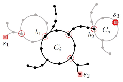
We say that a vertex $v\in V(C_{i})$ is branch-active if $\deg(v)\geq 4$ or $T_{v}$ contains a vertex of degree $\geq 3$ distinct from $v$. We denote the number of branch-active vertices on $C_{i}$ by $b(C_{i}).$ If a vertex $v$ from a cycle $C_{i}$ is branch-active, then $T_{v}$ contains both a pair of vertices and a pair of edges which are not distinguished by any vertex outside $T_{v}$, see Figure 1.

Now, we will introduce a property called ”branch-resolving” which a set of vertices $S\subseteq V(G)$ must possess in order to avoid this problem of non distinguished vertices (resp. edges) due to branching. First, a thread hanging at a vertex $v$ of degree $\geq 3$ is $S$-free if it does not contain a vertex from $S.$ Now, a set of vertices $S\subseteq V(G)$ is branch-resolving if at most one $S$-free thread is hanging at every vertex $v\in V(G)$ of degree $\geq 3$. Therefore, for every branch-resolving set $S$ it holds that $\left|S\right|\geq L(G)$ where

It is known in literature [11, 12] that for a tree $T$ it holds that $\mathrm{dim}(G)=\mathrm{edim}(G)=L(G).$

Also, given a set of vertices $S\subseteq V(G),$ we say that a vertex $v\in V(C_{i})$ is $S$-active if $T_{v}$ contains a vertex from $S.$ The number of $S$-active vertices on a cycle $C_{i}$ is denoted by $a_{S}(C_{i}).$ If $a_{S}(C_{i})\geq 2$ for every cycle $C_{i}$ in $G,$ then we say the set $S$ is biactive. For a biactive branch-resolving set $S$ the following holds: if a vertex $v$ from a cycle $C_{i}$ is branch-active, then $T_{v}$ contains a vertex with two threads hanging at it or $T_{v}$ contains a cycle, either way $T_{v}$ contains a vertex from $S,$ so $v$ is $S$-active. Therefore, for a biactive branch-resolving set $S$ we have $a_{S}(C_{i})\geq b(C_{i})$ for every $i$.

Assume now that $S$ is not biactive. We may assume that $G$ has at least one cycle, otherwise $G$ is a tree and there is nothing to prove. Notice that an empty set $S$ cannot be either a vertex or an edge metric generator in a cactus graph unless $G=K_{2}$ but then it is a tree. Therefore, if $S$ is not biactive, there must exist a cycle $C_{i}$ with precisely one $S$-active vertex $v$ and let $v_{1}$ and $v_{2}$ be the two neighbors of $v$ on $C_{i}.$ Then $v_{1}$ and $v_{2}$ (resp. $v_{1}v$ and $v_{2}v$) are not distinguished by $S,$ a contradiction.    

The above lemma gives us a necessary condition for $S$ to be a vertex (resp. an edge) metric generator in a cactus graph. In [19], a more elaborate condition for unicyclic graphs was established, which is both necessary and sufficient. In this paper we will extend that condition to cactus graphs, but to do so we first need to introduce the following definitions from [19]. Let $C_{i}$ be a cycle in a cactus graph $G$ and let $v_{i},$ $v_{j}$ and $v_{k}$ be three vertices of $C_{i},$ we say that $v_{i},$ $v_{j}$ and $v_{k}$ are a geodesic triple on $C_{i}$ if

It was shown in [18] that a biactive branch-resolving set with a geodesic triple of $S$-active vertices on every cycle is both a vertex and an edge metric generator. This result is useful for bounding the dimensions from above. Also, we need the definition of the five graph configurations from [19].

Let us now introduce five configurations which a cactus graph can contain with respect to a biactive branch-resolving set $S.$ All these configurations are illustrated by Figure 2.

Notice that only an even cycle can contain configuration $\mathcal{A}$ or $\mathcal{C}$. Also, configurations $\mathcal{B}$ and $\mathcal{D}$ are almost the same, they differ only if $C$ is odd where the index $i$ can take two more values in $\mathcal{D}$ than in $\mathcal{B}.$ Finally, for configurations $\mathcal{A}$, $\mathcal{C}$, and $\mathcal{E}$ it holds that $a_{S}(C)=2,$ so there are only two $S$-active vertices on the cycle $C$ and hence no geodesic triple of $S$-active vertices. On the other hand, for configurations $\mathcal{B}$ and $\mathcal{D}$ there might be more than two $S$-active vertices on the cycle $C,$ but the bounds $k\leq\left\lfloor g/2\right\rfloor-1$ and $k\leq\left\lceil g/2\right\rceil-1$ again imply there is no geodesic triple of $S$-active vertices on $C.$ Therefore, we can state the following observation which is useful for constructing metric generators.

The following result regarding configurations $\mathcal{A}$, $\mathcal{B}$, $\mathcal{C}$, $\mathcal{D}$, and $\mathcal{E}$ was established for unicyclic graphs (see Lemmas 6, 7, 13 and 14 from [19]).

In this paper we will extend this result to cactus graphs and then use it to determine the exact value of the vertex and the edge metric dimensions of such graphs. We first give an example how this approach with configurations can be extended to cactus graphs.

Besides this configuration approach, in cactus graphs an additional condition will have to be introduced for the situation when a pair of cycles share a vertex.

Let $G$ be a cactus graph with cycles $C_{1},\ldots,C_{c}.$ We say that a vertex $v\in V(G)$ gravitates to a cycle $C_{i}$ in $G$ if there is a path from $v$ to a vertex from $C_{i}$ which does not share any edge nor any internal vertex with any cycle of $G.$ A unicyclic region of the cycle $C_{i}$ from $G$ is the subgraph $G_{i}$ of $G$ induced by all vertices that gravitate to $C_{i}$ in $G.$ The notion of unicyclic region of a cactus graph is illustrated by Figure 4.

Notice that each unicyclic region $G_{i}$ is a unicyclic graph with its cycle being $C_{i}.$ Also, considering the example from Figure 4, one can easily notice that two distinct unicyclic regions may not be vertex disjoint, as the path connecting vertex $b_{2}$ and the cycle $C_{i}$ belongs both to $G_{i}$ and $G_{j}.$ But, it does hold that all unicyclic regions cover the whole $G.$ We say that a subgraph $H$ of a graph $G$ is an isometric subgraph if $d_{H}(u,v)=d_{G}(u,v)$ for every pair of vertices $u,v\in V(H).$ The following observation is obvious.

Finally, we say that a vertex $v$ from a unicyclic region $G_{i}$ is a boundary vertex if $v\in V(C_{j})$ for $j\not=i.$ In the example from Figure 4, the boundary vertices of the region $G_{i}$ are $b_{1}$ and $b_{2}$.

Let $S$ be a biactive branch-resolving set in $G$ and let $G_{i}$ be a unicyclic region in $G.$ For the set $S$ we define the regional set $S_{i}$ as the set obtained from $S\cap V(G_{i})$ by introducing all boundary vertices from $G_{i}$ to $S$. For example, in Figure 4 the set $S_{i}=\{s_{2},b_{1},b_{2}\}$ is the regional set in the region of the cycle $C_{i}$.

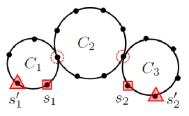
Notice that the condition from Lemma 7 is necessary for $S$ to be a metric generator, but it is not sufficient as is illustrated by the graph shown in Figure 5 in which every regional set $S_{i}$ is a vertex (resp. an edge) metric generator in the corresponding region $G_{i}$, but there still exists a pair of vertices (resp. edges) which is not distinguished by $S,$ so $S$ is not a vertex (resp. an edge) metric generator in $G$.

Next, we will introduce notions which are necessary to state a condition which will be both necessary and sufficient for a biactive branch-resolving set $S$ to be a vertex (resp. an edge) metric generator in a cactus graph $G.$ An $S$-path of the cycle $C_{i}$ is any subpath of $C_{i}$ which contains all $S$-active vertices on $C_{i}$ and is of minimum possible length. We denote an $S$-path of the cycle $C_{i}$ by $P_{i}$. Notice that the end-vertices of an $S$-path are always $S$-active, otherwise it would not be shortest. For example, on the cycle $C_{2}$ in Figure 5 there are two different paths connecting $S$-active vertices $v$ and $w,$ one is of the length $3$ and the other of length $5,$ so the shorter one is an $S$-path. Also, an $S$-path $P_{i}$ of a cycle $C_{i}$ may not be unique, as there may exist several shortest subpaths of $C_{i}$ containing all $S$-active vertices on $C_{i},$ but if the length of $P_{i}$ satisfies $\left|P_{i}\right|\leq\left\lceil g_{i}/2\right\rceil-1$ then $P_{i}$ is certainly unique and its end-vertices are $v_{0}$ and $v_{k}$ in the canonical labelling of $C_{i}.$

Notice that the notion of a vertex-critical and an edge-critical vertex differs only on odd cycles. We say that two distinct cycles $C_{i}$ and $C_{j}$ of a cactus graph $G$ are vertex-critically incident (resp. edge-critically incident) with respect to $S$ if $C_{i}$ and $C_{j}$ share a vertex $v$ which is vertex-critical (resp. edge-critical) with respect to $S$ on both $C_{i}$ and $C_{j}$. Notice that on odd cycles the required length of an $S$-path $P_{i}$ for $v$ to be vertex-critical differs from the one required for $v$ to be edge-critical, while on even cycles the required length is the same.

To illustrate this notion, let us consider the cycle $C_{2}$ in the graph from Figure 5. Vertices $v$ and $w$ are both vertex-critical and edge-critical on $C_{2}$ with respect to $S$ from the figure. Vertex $v$ belongs also to $C_{1}$ and it is also both vertex- and edge-critical on $C_{1}.$ Therefore, cycles $C_{1}$ and $C_{2}$ are both vertex- and edge-critically incident, the consequence of which is that a pair of vertices $v_{1}$ and $v_{2}$ which are neighbors of $v$ and a pair of edges $v_{1}v$ and $v_{2}v$ which are incident to $v$ are not distinguished by $S.$ On the other hand, vertex $w$ belongs also to $C_{3}$ on which it is edge-critical, but it is not vertex-critical since $P_{3}$ is not short enough. So, $C_{2}$ and $C_{3}$ are edge-critically incident, but not vertex-critically incident. Consequently, a pair of edges $w_{1}w$ and $w_{2}w$ is not distinguished by $S,$ but a pair of vertices $w_{1}$ and $w_{2}$ is distinguished by $S.$ We will show in the following lemma that this holds in general.

Each of Lemmas 7 and 9 gives a necessary condition for a biactive branch-resolving set $S$ to be a vertex (resp. an edge) metric generator in a cactus graph $G$. Let us now show that these two necessary conditions taken together form a sufficient condition for $S$ to be a vertex (resp. an edge) metric generator.

If $d(x,b)<d(x^{\prime},b),$ let $v_{k}$ be an $S$-active vertex on $C_{i}$ distinct from $b,$ which must exist as $S$ is biactive. From (1) we obtain

so similarly as in previous subcase $x$ and $x^{\prime}$ are distinguished by a vertex $s_{k}\in S$ which belongs to the connected component of $G-E(C_{i})$ which contains $v_{k}.$

Therefore, assume that $d(x,b)=d(x^{\prime},b).$ If a shortest path from $x$ to all $S$-active vertices on $C_{i}$ and a shortest path from $x^{\prime}$ to all $S$-active vertices on $C_{l}$ leads through $b,$ then $x^{\prime}$ belongs to $C_{l},$ i.e. $j=l$, and the pair of cycles $C_{i}$ and $C_{l}$ are vertex-critically (resp. edge-critically) incident, a contradiction. So, we may assume there is an $S$-active vertex $v_{k}$, say on $C_{i}$, such that a shortest path from $x$ to $v_{k}$ does not lead through $b.$ Therefore,

But now, similarly as in previous cases we have that $x$ and $x^{\prime}$ are distinguished by a vertex $s_{k}\in S$ which is contained in the connected component of $G-E(C_{i})$ containing $v_{k}.$    

Let us now relate these results with configurations $\mathcal{A},$ $\mathcal{B}$, $\mathcal{C}$, $\mathcal{D}$ and $\mathcal{E}$.

Notice that Lemmas 7, 9 and 10 give us a condition for $S$ to be a vertex (resp. an edge) metric generator in a cactus graph, which is both necessary and sufficient. In the light of Lemma 11, we can further apply Theorem 5 to obtain the following result which unifies all our results.

The other direction is the consequence of Lemma 10 and Theorem 5.    

Let $G$ be a cactus graph and $S$ a smallest biactive branch-resolving set in $G.$ Then

where $B(G)=\sum_{i=1}^{c}\max\{0,2-b(C_{i})\}.$ If $b(C_{i})\geq 2$, then the set of $S$-active vertices on $C_{i}$ is the same for all smallest biactive branch-resolving sets $S$. The set of $S$-active vertices may differ only on cycles $C_{i}$ with $b(C_{i})<2.$ Therefore, such a cycle $C_{i}$ may contain one of the configurations with respect to one smallest biactive branch-resolving set, but not with respect to another. This is illustrated by Figure 6.

For two distinct smallest biactive branch-resolving sets $S$, the set of $S$-active vertices may differ only on cycles with $b(C_{i})\leq 1.$ Let $C_{i}$ and $C_{j}$ be two such cycles in $G$ and notice that the choice of the vertices included in $S$ from the region of $C_{i}$ is independent of the choice from $C_{j}.$ Therefore, there exists at least one smallest biactive branch-resolving set $S$ such that every $\mathcal{ABC}$-negative (resp. $\mathcal{ADE}$-negative) avoids the three configurations with respect to $S.$ Notice that there may exist more than one such set $S,$ and in that case they all have the same size, so among them we may choose the one with the smallest number of vertex-critical (resp. edge-critical) incidencies. Therefore, we say that a smallest biactive branch-resolving set $S$ is nice if every $\mathcal{ABC}$-negative (resp. $\mathcal{ADE}$-negative) cycle $C_{i}$ does not contain the three configurations with respect to $S$ and the number of vertex-critically (resp. edge-critically) incident pairs of cycles with respect to $S$ is the smallest possible. The niceness of a smallest biactive branch-resolving set is illustrated by Figure 7.

A set $S\subseteq V(G)$ is a vertex cover if it contains a least one end-vertex of every edge in $G.$ The cardinality of a smallest vertex cover in $G$ is the vertex cover number denoted by $\tau(G).$ Now, let $G$ be a cactus graph and let $S$ be a nice smallest biactive branch-resolving set in $G.$ We define the vertex-incident graph $G_{vi}$ (resp. edge-incident graph $G_{ei}$) as a graph containing a vertex for every cycle in $G,$ where two vertices are adjacent if the corresponding cycles in $G$ are $\mathcal{ABC}$-negative and vertex-critically incident (resp. $\mathcal{ADE}$-negative and edge-critically incident) with respect to $S$. For example, if we consider the cactus graph $G$ from Figure 8, then $V(G_{vi})=V(G_{ei})=\{C_{i}:i=1,\ldots,7\},$ where $E(G_{vi})=\{C_{3}C_{4},C_{4}C_{5}\}$ and $E(G_{ei})=\{C_{2}C_{3},C_{3}C_{4},C_{4}C_{5}\}.$

We are now in a position to establish the following theorem which gives us the value of the vertex and the edge metric dimensions in a cactus graph.

Let $S$ be a smallest vertex (resp. edge) metric generator in $G$. Due to Lemma 1 the set $S$ must be branch-resolving. Let $S_{1}\subseteq S$ be a smallest branch-resolving set contained in $S,$ so $\left|S_{1}\right|=L(G).$ Since according to Lemma 1 the set $S$ must also be biactive, let $S_{2}\subseteq S\backslash S_{1}$ be a smallest set such that $S_{1}\cup S_{2}$ is biactive. Obviously, $S_{1}\cap S_{2}=\phi$ and $\left|S_{2}\right|=B(G).$

Since $S_{1}\cup S_{2}$ is a smallest biactive branch-resolving set in $G,$ it follows that every $\mathcal{ABC}$-positive (resp. $\mathcal{ADE}$-positive) cycle in $G$ contains at least one of the three configurations with respect to $S_{1}\cup S_{2},$ so according to Theorem 12 the set $S_{1}\cup S_{2}$ is not a vertex (resp. an edge) metric generator in $G.$ Therefore, each $\mathcal{ABC}$-positive (resp. $\mathcal{ADE}$-positive) cycle $C_{i}$ must contain a vertex $s_{i}\in S\backslash(S_{1}\cup S_{2}),$ where we may assume that $s_{i}$ is chosen so that it forms a geodesic triple on $C_{i}$ with vertices from $S_{1}\cup S_{2},$ so according to Observation 4 the cycle $C_{i}$ will not contain any of the configurations with respect to $S.$ Denote by $S_{3}$ the set of vertices $s_{i}$ from every $\mathcal{ABC}$-positive (resp. $\mathcal{ADE}$-positive) cycle in $G.$ Obviously, $S_{3}\subseteq S,$ $S_{1}\cap S_{2}\cap S_{3}=\phi$ and $\left|S_{3}\right|=c_{\mathcal{ABC}}(G)$ (resp. $\left|S_{3}\right|=c_{\mathcal{ADE}}(G)$).

Notice that $S_{1}\cup S_{2}\cup S_{3}$ is a biactive branch-resolving set in $G$ such that every cycle $C_{i}$ in $G$ does not contain any of the configurations $\mathcal{A},$ $\mathcal{B},$ $\mathcal{C}$ (resp. $\mathcal{A},$ $\mathcal{D},$ $\mathcal{E}$) with respect to it. Notice that $S_{1}\cup S_{2}\cup S_{3}$ still may not be a vertex (resp. an edge) metric generator, as there may exist vertex-critically (resp. edge-critically) incident cycles in $G$ with respect to $S_{1}\cup S_{2}\cup S_{3}.$ Since $S$ is a smallest vertex (resp. edge) metric generator, we may assume that $S_{2}$ is chosen so that a smallest biactive branch-resolving set $S_{1}\cup S_{2}$ is nice. Therefore, the graph $G_{vi}$ (resp. $G_{ei}$) contains an edge for every pair of cycles in $G$ which are $\mathcal{ABC}$-negative and vertex-critically incident (resp. $\mathcal{ADE}$-negative and edge-critically incident) with respect to $S_{1}\cup S_{2}.$ Let us denote $S_{4}=S\backslash(S_{1}\cup S_{2}\cup S_{3}).$ For each edge $xy$ in $G_{vi}$ (resp. $G_{ei}$) the set $S_{4}$ must contain a vertex from $C_{x}$ or $C_{y},$ chosen so that it forms a geodesic triple of $S$-active vertices on $C_{x}$ or $C_{y}$ with other vertices from $S.$ Therefore, $S_{4}$ must contain at least $\tau(G_{vi})$ (resp. $\tau(G_{ei})$) vertices in order for $S$ to be a vertex (resp. an edge) metric generator. Since $S$ is a smallest vertex (resp. edge) metric generator, it must hold $\left|S_{4}\right|=\tau(G_{vi})$ (resp. $\left|S_{4}\right|=\tau(G_{ei})$).

References

- [1] P. S. Buczkowski, G. Chartrand, C. Poisson, P. Zhang, On -dimensional graphs and their bases, Period. Math. Hungar. 46(1) (2003) 9–15.
- [2] J. Caceres, C. Hernando, M. Mora, I. M. Pelayo, M. L. Puertas, C. Seara, D. R. Wood, On the metric dimension of Cartesian products of graphs, SIAM J. Discrete Math. 21(2) (2007) 423–441.
- [3] G. Chartrand, L. Eroh, M. A. Johnson, O. R. Oellermann, Resolvability in graphs and the metric dimension of a graph, Discrete Appl. Math. 105 (2000) 99–113.
- [4] L. Eroh, C.X. Kang, E. Yi, A comparison between the metric dimension and zero forcing number of trees and unicyclic graphs, Acta Math. Sin. (Engl. Ser.) 33(6) (2017) 731–747.
- [5] M. Fehr, S. Gosselin, O. R. Oellermann, The metric dimension of Cayley digraphs, Discrete Math. 306 (2006) 31–41.
- [6] J. Geneson, Metric dimension and pattern avoidance in graphs, Discrete Appl. Math. 284 (2020) 1–7.
- [7] F. Harary, R. A. Melter, On the metric dimension of a graph, Ars Combin. 2 (1976) 191–195.
- [8] Y. Huang, B. Hou, W. Liu, L. Wu, S. Rainwater, S. Gao, On approximation algorithm for the edge metric dimension problem, Theoret. Comput. Sci. (2020), doi:https://doi.org/10.1016/j.tcs.2020.05.005.
- [9] A. Kelenc, Distance-Based Invariants and Measures in Graphs, PhD thesis, University of Maribor, Faculty of Natural Sciences and Mathematics, 2020.
- [10] A. Kelenc, D. Kuziak, A. Taranenko, I. G. Yero, Mixed metric dimension of graphs, Appl. Math. Comput. 314(1) (2017) 42–438.
- [11] A. Kelenc, N. Tratnik, I. G. Yero, Uniquely identifying the edges of a graph: the edge metric dimension, Discrete Appl. Math. 251 (2018) 204–220.
- [12] S. Khuller, B. Raghavachari, A. Rosenfeld, Landmarks in graphs, Discrete Appl. Math. 70 (1996) 217–229.
- [13] D. J. Klein, E. Yi, A comparison on metric dimension of graphs, line graphs, and line graphs of the subdivision graphs, Eur. J. Pure Appl. Math. 5(3) (2012) 302–316.
- [14] M. Knor, S. Majstorović, A. T. M. Toshi, R. Škrekovski, I. G. Yero, Graphs with the edge metric dimension smaller than the metric dimension, Appl. Math. Comput. 401 (2021) 126076.
- [15] R. A. Melter, I. Tomescu, Metric bases in digital geometry, Comput. Vis. Graph. Image Process. 25 (1984) 113–121.
- [16] I. Peterin, I. G. Yero, Edge metric dimension of some graph operations, Bull. Malays. Math. Sci. Soc. 43 (2020) 2465–2477.
- [17] S. W. Saputro, R. Simanjuntak, S. Uttunggadewa, H. Assiyatun, E. T. Baskoro, A. N. M. Salman, M. Bača, The metric dimension of the lexicographic product of graphs, Discrete Math. 313 (2013) 1045–1051.
- [18] J. Sedlar, R. Škrekovski, Bounds on metric dimensions of graphs with edge disjoint cycles, Appl. Math. Comput. 396 (2021) 125908.
- [19] J. Sedlar, R. Škrekovski, Vertex and edge metric dimensions of unicyclic graphs, arXiv:2104.00577 [math.CO].
- [20] J. Sedlar, R. Škrekovski, Extremal mixed metric dimension with respect to the cyclomatic number, Appl. Math. Comput. 404 (2021) 126238.
- [21] J. Sedlar, R. Škrekovski, Mixed metric dimension of graphs with edge disjoint cycles, Discr. Appl. Math. 300 (2021) 1–8.
- [22] P. J. Slater, Leaves of trees, Congr. Numer. 14 (1975) 549–559.
- [23] I. G. Yero, D. Kuziak, J. A. Rodriguez-Velazquez, On the metric dimension of corona product graphs, Comput. Math. Appl. 61 (2011) 2793–2798.
- [24] Y. Zhang, S. Gao, On the edge metric dimension of convex polytopes and its related graphs, J. Comb. Optim. 39(2) (2020) 334–350.
- [25] E. Zhu, A. Taranenko, Z. Shao, J. Xu, On graphs with the maximum edge metric dimension, Discrete Appl. Math. 257 (2019) 317–324.
- [26] N. Zubrilina, On the edge dimension of a graph, Discrete Math. 341(7) (2018) 2083–2088.