Varying Coefficient Model via Adaptive Spline Fitting

In varying coefficient models, each coefficient $\beta_{j}(u)$ is a function of the conditional variable $u$, which can be estimated by fitting a polynomial spline on $u$. In this paper we assume that $u$ is a univariate variable. Let $X_{i}=(x_{i,1},\ldots,x_{i,p})^{T}\in\mathbf{R}^{p}$, $u_{i}$, and $y_{i}$ denote the $i$th observations of the predictor vector, the conditional variable, and the response variable, respectively, for $i=1,\ldots,n$. Suppose the knots are common to all coefficients located at $d_{1}<\ldots<d_{L}$, and the corresponding B-splines of degree $D$ are $B_{k}(u)\ (k=1,\ldots,D+L+1)$. Each varying coefficient can be represented as $\beta_{j}(u)=\sum_{k=1}^{D+L+1}c_{j,k}B_{k}(u)$, where the coefficients $c_{j,k}$ are estimated by minimizing the following sum of squared errors:

$$\sum_{i=1}^{n}\left\{y_{i}-\sum_{j=1}^{p}x_{i,j}\sum_{k=1}^{D+L+1}c_{j,k}B_{k}(u_{i})\right\}^{2}.$$

(1)

In previous work, the knots for polynomial spline were always chosen as equidistant quantiles of $u$ and are the same for all predictors. The approach is computationally straightforward, but the knots chosen cannot properly reflect the varying smoothness between and within the coefficients. We propose an adaptive knot selection approach in which the knots can be interpreted as turning points of the coefficients.

For knots $d_{1}<\ldots<d_{L}$, we define the segmentation scheme $S=\{s_{1},\ldots,s_{L+1}\}$ for the observed samples ordered by $u$, where $s_{k}=\{i\mid d_{k}<u_{i}\leq d_{k+1}\}$, with $d_{0}=-\infty$ and $d_{L+1}=\infty$. If the true coefficients $\beta(u)=(\beta_{1}(u),\ldots,\beta_{p}(u))^{T}\in\mathbf{R}^{p}$ is a linear function of $u$ within each segment, i.e., $\beta(u)=a_{s}+b_{s}u$ for $a_{s},b_{s}\in\mathbf{R}^{p}$, then the observed response satisfies

$$y=a_{s}^{T}X+b_{s}^{T}(uX)+\epsilon,\epsilon\sim N(0,\sigma_{s}^{2}).$$

(2)

Thus, the coefficients can be estimated by maximizing the log-likelihood function, which is equivalent to minimizing the loss function:

$$L(S)=\sum_{s\in S}|s|\log\hat{\sigma}^{2}_{s},$$

(3)

where $\hat{\sigma}^{2}_{s}$ is the residual variance by regressing $y_{i}$ over $(X_{i},u_{i}X_{i})$ for $i\in s$.

Because any almost-everywhere continuous function can be approximated by piece-wise linear functions, we can employ the estimating framework in (2) and derive (3). To avoid over-fitting when maximizing the log-likelihood over the parameters and segmentation schemes, we constrain that $|s|$ is greater than a lower bound $m_{s}=n^{-\alpha}\ (\alpha>0)$, and penalize the loss function with the number of segments

$$L(S,\lambda_{0})=\sum_{s\in S}|s|\log\hat{\sigma}^{2}_{s}+\lambda_{0}|S|\log(n),$$

(4)

where $\lambda_{0}>0$ is the penalty strength. The resulting knots correspond to the segmentation scheme $S$ that minimizes the penalized loss function (4). When $\lambda_{0}$ is very large, this strategy tends to select no knots, whereas when $\lambda_{0}$ gets close to 0 it can select as many knots as $n^{1-\alpha}$. We find the optimal $\lambda_{0}$ by minimizing the Bayesian information criterion (Schwarz et al.,, 1978) of the fitted model. For a given $\lambda_{0}$, suppose $L(\lambda_{0})$ knots are finally proposed, and the fitted model is $\hat{f}(X,u)$. Then, we have

$$\textsc{bic}(\lambda_{0})=n\log\left[\frac{1}{n}\sum_{i=1}^{n}\{y_{i}-f(X_{i},u_{i})\}^{2}\right]+p\{L(\lambda_{0})+D+1\}\log(n).$$

(5)

The optimal $\lambda_{0}$ is selected by searching over a grid to minimize bic$(\lambda_{0})$. We call this procedure the global adaptive knots selection strategy as it assumes that all the predictors have the same set of knots. We will discuss in Section 2.4 how to allow each predictor to have its own set of knots.

Here we only use the piece-wise linear model (2) and loss function (4) for knots selection, but will fit the varying coefficients with B-splines derived from the resulting knots via minimizing (1). In this way, the fitted varying coefficients are smooth functions and the smoothness is determined by the degree of the splines. This method is referred to as the global adaptive spline fitting throughout the paper.

The proposed method is invariant to marginal distribution of $u$. Without loss of generality, we assume that $u$ follows the uniform distribution in $[0,1]$. According to Definition 1 below, a turning point of $u$, denoted as $c_{k}$, is defined as a local maximum or minimum of any coefficient $\beta_{i}(u)\ (j=1,\ldots,p)$. In Theorem 1, we show that the adaptive knots selection approach can almost surely detect all the turning points of $\beta(u)$.

Although the adaptive spline fitting method is motivated by a piece-wise linear model, Theorem 1 shows that with probability approaching 1, we can detect all the turning points accurately under general varying coefficient functions. The selected knots could be a superset of the real turning points especially when $\lambda_{0}$ is small, so we tune $\lambda_{0}$ with bic (5) which penalizes the number of selected knots, to find the optimal set.

When the varying coefficient functions are piece-wise linear, each coefficient $\beta_{j}(u)\ (j=1,\ldots,p)$ can be almost surely defined as

$\displaystyle\beta_{j}(u)=a_{j,k}+b_{j,k}u,\quad c_{j,k-1}<u\leq c_{j,k},\quad k=1,\ldots,K_{j}+1,$

where $c_{j,0}=0$, $c_{j,K_{j}+1}=1$ and $(a_{j,k}-a_{j,k+1})^{2}+(b_{j,k}-b_{j,k+1})^{2}>0\ (k=1,\ldots,K_{j})$ if $K_{j}\geq 1$. When $K_{j}=0$ the varying coefficient $\beta_{j}(u)$ is a simple linear function of $u$, otherwise we call $c_{j,k}\ (k=1,\ldots,K_{j})$ the change points for coefficients $\beta_{j}(u)$, because the linear relationship varies before and after these points. Then $\bigcup_{K_{j}\geq 1}\{c_{j,1},\ldots,c_{j,K_{j}}\}$ are all the change points of the entire varying coefficient function. In Theorem 2, we show that the adaptive knots selection method can almost surely discover the change points of $\beta(u)$ without false positive selection.

The theorem shows that if the varying coefficient function is piece-wise linear, the method can discover all the change points with almost 100% accuracy.

The brute force algorithm to compute the optimal knots has a computation complexity of $O(2^{n})$ and is impractical. As summarized by the following algorithm, we propose a dynamic programming approach whose computation complexity is of order $O(n^{2})$. If we further assume that the knots can only be chosen from a predetermined set $\mathcal{M}$, e.g. $\frac{m}{\sqrt{n}}\ (m=1,\ldots,\lfloor\sqrt{n}\rfloor-1)$ quantiles of $u_{i}$’s, the computation complexity can be further reduced to $O(|\mathcal{M}|^{2})$. Note that the algorithm in Section 2.4 of Wang et al., (2017) is a special case with a constant $x$. The algorithm is summarized in the following three steps:

1. 1.

   Data preparation: Arrange the data $(X_{i},u_{i},y_{i})\ (i=1,\ldots,n)$ according to order of $u_{i}$ from small to large. Without lose of generality, we assume that $u_{1}<\cdots<u_{n}$.

2. 2.

   Obtain the minimum loss by forward recursion: Define $m_{s}=\lceil n^{-\alpha}\rceil\ (\alpha>0)$ as the smallest segment size, and set $\lambda=\lambda_{0}\log(n)$. Initialize two sequence: $(\mathrm{Loss}_{i},\mathrm{Prev}_{i})\ (i=1,\ldots n)$ with $\mathrm{Loss}_{0}=0$. For $i=m_{s},\ldots,n$, recursively fill in entries of the tables with

   $$\mathrm{Loss}_{i}=\min_{i^{\prime}\in I_{i}}(\mathrm{Loss}_{i^{\prime}-1}+l_{i^{\prime}:i}+\lambda),\quad\mathrm{Prev}_{i}=\operatorname*{arg\,min}_{i^{\prime}\in I_{i}}(\mathrm{Loss}_{i^{\prime}-1}+l_{i^{\prime}:i}+\lambda).$$

   Here $I_{i}=\{1\}\cup\{m_{s}+1,\ldots,i-m_{s}+1\}$ and $l_{i^{\prime}:i}=(i-i^{\prime}+1)\log\hat{\sigma}^{2}_{i^{\prime}:i}$ where $\hat{\sigma}^{2}_{i^{\prime}:i}$ is the residual variance of regressing $y_{k}$ on $(X_{k},u_{k}X_{k})\ (k=i^{\prime},\ldots,i)$.

3. 3.

   Determine knots by backward tracing: Let $p=\mathrm{Prev}_{n}$. If $p=1$ no knot is needed; otherwise, we recursively add $0.5(u_{p-1}+u_{p})$ as a new knot with $p=\mathrm{Prev}_{p}$ until $p=1$.

When the algorithm is run with a grid of $\lambda_{0}$, we repeat Step 2 and 3 for all the $\lambda_{0}$’s, and return the final model with the minimum bic.

The global adaptive knots selection method introduced in Section 2.1 assumes that the set of knot locations are the same for all predictors, similar to most of the literature for polynomial spline fitting. However, different coefficients may have a different resolution of smoothness relative to $u$, and a different set of knots for each predictor is preferable. Here we propose a predictor-specific adaptive spline fitting algorithm on top of the global knot selection. Suppose the fitted model for the global adaptive spline fitting is $\hat{f}(X,u)=\sum_{j=1}^{p}\hat{\beta}_{j}(u)x_{j}$. For predictor $j$, the knots can be updated by performing the same knots selection procedure between it and the residual without it, that is

$$r_{i}=y_{i}-\sum_{j^{\prime}\neq j}\hat{\beta}_{j^{\prime}}(u_{i})x_{i,j^{\prime}},\quad i=1,\ldots,n.$$

(6)

If bic in (5) is smaller for the corresponding new polynomial spline model with the new knots, the knots and fitted model are update. The steps are repeated until bic cannot be further minimized. The following three steps summarizes the algorithm:

1. 1.

   global adaptive spline: Run the global adaptive spline fitting algorithm for $(X_{i},u_{i},y_{i})\ (i=1,\ldots,n)$. Denote $\hat{f}(X,u)$ as the fitted model and compute model bic with (5).

2. 2.

   Update knots with bic: For $j=1,\dots,p$, compute residual variable $r_{i}$ by (6). Run the global adaptive spline fitting algorithm for the residual and predictor $j$, that is $(x_{i,j},u_{i},r_{i})\ (i=1,\ldots,n)$. Denote the new fitted model as $\hat{f}^{j}(X,u)$ and corresponding bic as $\textsc{bic}_{j}$. Note that when we assume different number of knots for each predictor, the term $p\{L(\lambda_{0})+D+1\}\log(n)$ in (5) should be replaced by $\left\{\sum_{j=1}^{p}L_{j}(\lambda_{0})+p(D+1)\right\}\log(n)$, where $L_{j}(\lambda_{0})$ is the number of knots for predictor $j$.

3. 3.

   Recursively update model: If $\min\textsc{bic}_{j}<\textsc{bic}$ and $j^{*}=\operatorname*{arg\,min}\textsc{bic}_{j}$, update the current model by $\hat{f}(X,u)=\hat{f}^{j^{*}}(X,u)$, and repeat Step 3. Otherwise return the fitted model $\hat{f}(X,u)$.

An alternative approach to model the heterogeneous relationships between coefficients is to replace the initial model in Step 1 with $\hat{f}(X,u)=0$, and repeat the following two steps. However, starting from the global model is preferred because fitting to residual instead of the original response minimizes the mean squared error more efficiently. Simulation studies in Section 3 show that the predictor-specific knots can further reduce mean squared error for the fitted coefficient, compared with the global knot selection approach.

When the number of predictors is large and the number of predictors with non-zero varying coefficients is small, we perform a variable selection for all the predictors. For predictor $j$, we run the knots selection procedure between it and the response, and construct B-spline functions as $\{B_{j,k}(u)\}\ (L=1,\ldots,L_{j}+D+1)$ where $L_{j}$ is the number of knots and $D$ is the degree of the B-splines. Then, we perform the variable selection method for varying coefficient model proposed by Wei et al., (2011), which is a generalization of group LASSO (Yuan & Lin,, 2006) and adaptive LASSO (Zou,, 2006). Wei et al., (2011) shows that group LASSO tends to over select variables and suggests adaptive group LASSO for variable selection. In their original algorithm, the knots for each predictor are chosen as equidistant quantiles and not predictor-specific. The following three steps summarize our proposed algorithm:

1. 1.

   Select knots for each predictor: Run the global adaptive spline fitting algorithm between each predictor $x_{i,j}$ and response $y_{i}$. Denote the corresponding B-splines as $B_{j,k}(u)\ (k=1,\ldots,L_{j}+D+1)$ where $L_{j}$ is the number of knots for predictor $j$ and $D$ is degree of splines.

2. 2.

   Group LASSO for first step variable selection: Run group LASSO algorithm for the following loss function

   $\displaystyle\frac{1}{n}\sum_{i=1}^{n}\left\{y_{i}-\sum_{j=1}^{p}x_{i,j}\sum_{k=1}^{L_{j}+D+1}c_{j,k}B_{j,k}(u_{i})\right\}+\lambda_{1}\sum_{j=1}^{p}(c_{j}^{\prime}R_{j}c_{j})^{1/2},\quad\lambda_{1}>0$

   where $c_{j}=(c_{j,1},\ldots,c_{j,L_{j}+D+1})$ and $R_{j}$ is the kernel matrix whose $(k_{1},k_{2})$ element is $E\{B_{j,k_{1}}(u)*B_{j,k_{2}}(u)\}$. Denote the fitted coefficients as $\tilde{c}_{j,k}$.

3. 3.

   Adaptive group LASSO for second step variable selection: Run adaptive group LASSO algorithm for the updated loss function

   $\displaystyle\frac{1}{n}\sum_{i=1}^{n}\left\{y_{i}-\sum_{j=1}^{p}x_{i,j}\sum_{k=1}^{L_{j}+D+1}c_{j,k}B_{j,k}(u_{i})\right\}+\lambda_{2}\sum_{j=1}^{p}w_{j}(c_{j}^{\prime}R_{j}c_{j})^{1/2},\quad\lambda_{2}>0$

   with weight as $w_{k}=\infty$ if $\tilde{c}_{j}^{\prime}R_{j}\tilde{c}_{j}=0$, otherwise $w_{k}=(\tilde{c}_{j}^{\prime}R_{j}\tilde{c}_{j})^{-1/2}$. Denote the fitted coefficients as $\hat{c}_{j,k}$ and the selected variables are those with $\hat{c}_{j}^{\prime}R_{j}\hat{c}_{j}\neq 0$.

For Steps 2 and 3, parameter $\lambda_{1}$ and $\lambda_{2}$ are chosen by minimizing bic (5) for the fitted model, where the degree of freedom is computed with only the selected predictors. Simulation studies in Section 3.2 show that, with the knots selection Step 1, the algorithm can always choose the correct predictors with a reasonable number of samples.

In this section, we compare the global and predictor-specific adaptive spline fitting approaches we introduced with the equidistant spline fitting approach as well as a commonly used kernel method package tvReg by Casas & Fernandez-Casal, (2019), using the simulation examples from Tang & Cheng, (2012). The model simulates a longitudinal data, which are frequently encountered in biomedical applications. In this example, the conditional random variable represents time and for convenience, we use notation $t$ instead of $u$. We simulated $n$ individuals, each having a scheduled time set $\{0,1,\ldots,19\}$ to generate observations. A scheduled time can be skipped with probability 0.6, so no observation will be generated at the skipped time. For each non-skipped scheduled time, the real observed time is the scheduled time plus a random disturbance from $\mathrm{Unif}(0,1)$. Consider the time-dependent predictors $X(t)=(x_{1}(t),x_{2}(t),x_{3}(t),x_{4}(t))^{T}$ with

	$\displaystyle x_{1}(t)=1,$		$\displaystyle x_{2}(t)\sim\mathrm{Bern}(0.6),$
	$\displaystyle x_{3}(t)\sim\mathrm{Unif}(0.1t,2+0.1t),$		$\displaystyle x_{4}(t)~{}\mid~{}x_{3}(t)\sim N\left(0,\frac{1+x_{3}(t)}{2+x_{3}(t)}\right).$

The response for individual $i$ at observed time $t_{i,k}$ is $y_{i}(t_{i,k})=\sum_{j=1}^{4}\beta_{j}(t_{i,k})x_{i,j}(t_{i,k})+\epsilon_{i}(t_{i,k})$, with

	$\displaystyle\beta_{1}(t)=1+3.5\sin(t-3),$		$\displaystyle\beta_{2}(t)=2-5\cos(0.75t-0.25),$
	$\displaystyle\beta_{3}(t)=4-0.04(t-12)^{2},$		$\displaystyle\beta_{4}(t)=1+0.125t+4.6\left(1-0.1t\right)^{3}.$

The random error $\epsilon_{i}(t_{i,k})$ are independent from the predictors, and generated with two components

$$\epsilon_{i}(t_{i,k})=v_{i}(t_{i,k})+e_{i}(t_{i,k}),$$

where $e_{i}(t_{i,k})\stackrel{{\scriptstyle i.i.d.}}{{\sim}}N(0,4)$, and $v_{i}(t_{i,k})\sim N(0,4)$ with correlation structure

$$\mathrm{cor}\left\{v_{i_{1}}(t_{i_{1},k_{1}}),v_{i_{2}}(t_{i_{2},k_{2}})\right\}=I(i_{1}=i_{2})\exp(-|t_{i_{1},k_{1}}-t_{i_{2},k_{2}}|).$$

Random errors are positively correlated within the same individual and are independent between different individuals. Figure 1 shows the true coefficients and the fitted coefficients by the equidistant and predictor-specific spline fitting methods for an example with $n=200$, as well as the selected knots. Note that for the equidistant fitting approach, the number of knots is also determined by minimizing the model bic (5). We observe that the fitted coefficients by the predictor-specific method are smoother than those by the equidistant method, especially for the less volatile coefficients $\beta_{3}(t)$ and $\beta_{4}(t)$. This is because the predictor-specific method uses only 1 knot for these two coefficient which better reflects the resolution, while the equidistant method uses 7 knots.

We compare the three methods by the mean square errors of their estimated coefficients, i.e.,

$$\textsc{mse}_{j}=\frac{1}{N}\sum_{i=1}^{n}\sum_{k=1}^{n_{i}}\frac{\left\{\hat{\beta}_{j}(t_{i,k})-\beta_{j}(t_{i,k})\right\}^{2}}{\mathrm{range}(\beta_{j})^{2}},$$

(7)

where ${\beta}_{j}(t)$ and $\hat{\beta}_{j}(t)$ are the true and estimated coefficients, respectively, $n_{i}$ is the total number of observations for individual $i$ and $N=\sum_{i=1}^{n}n_{i}$. We run the simulation with $n=200$ for 1000 repetitions. For adaptive spline methods we only consider knots from $\frac{m}{\sqrt{N}}\ (m=1,\ldots,\lfloor\sqrt{N}\rfloor)$ quantiles of $t_{i,k}$.

Table 1 shows the average $\textsc{mse}_{j}$ for the proposed global and predictor-specific methods, in comparison with the equidistant spline fitting and the kernel method. We find that the predictor-specific method has the smallest $\textsc{mse}_{j}$ for all four coefficients, significantly outperforming the other two methods. Interestingly, the equidistant method selects on average 6.9 knots, the global adaptive method selects on average 6.1 global knots for all predictors, whereas the predictor-specific method selects fewer on average: 5.8 knots for $x_{1}(t)$, 4.2 for $x_{2}(t)$, 1.5 for $x_{3}(t)$ and 0.8 for $x_{4}(t)$. The result is expected since $\beta_{3}(t)$ and $\beta_{4}(t)$ are less volatile than $\beta_{1}(t)$ and $\beta_{2}(t)$. It appears that the predictor-specific procedure can use a smaller number of knots to achieve a better fitting than the other two methods.

We use the simulation example from Wei et al., (2011) to compare the performance of our method with one using adaptive group LASSO and equidistant knots. Similar to the previous subsection, there are $n$ individuals, each having a scheduled time set $\{0,1,\ldots,29\}$ to generate observations and a skipping probability of 0.6. For each non-skipped scheduled time, the real observed time is the scheduled time adding a random disturbance generated from $\mathrm{Unif}(0,1)$. We construct $p=500$ time-dependent predictors as follows:

	$\displaystyle x_{1}(t)\sim\mathrm{Unif}\left(0.05+0.1t,2.05+0.1t\right),$		$\displaystyle x_{j}(t)~{}\mid~{}x_{1}(t)\sim N\left(0,\frac{1+x_{1}(t)}{2+x_{1}(t)}\right),\quad j=2,\ldots,5$
	$\displaystyle x_{6}(t)\sim N\left(3\exp\{(t+0.5)/30\},1\right)$		$\displaystyle x_{j}(t)\stackrel{{\scriptstyle i.i.d.}}{{\sim}}N(0,4),\quad j=7,\ldots,500.$

The same individual’s predictors $x_{j}(t)\ (j=7,\ldots,500)$ are correlated with $\mathrm{cor}\{x_{j}(t),x_{j}(s)\}=\exp(-|t-s|)$. The response for individual $i$ at observed time $t_{i,k}$ is $y_{i}(t_{i,k})=\sum_{j=1}^{6}\beta_{j}(t_{i,k})x_{i,j}(t_{i,k})+\epsilon_{i}(t_{i,k})$. The time-varying coefficients $\beta_{j}(t)\ (j=1,\ldots,6)$ are

	$\displaystyle\beta_{1}(t)=15+20\sin\{\pi(t+0.5)/15\},$		$\displaystyle\beta_{2}(t)=15+20\cos\{\pi(t+0.5)/15\},$
	$\displaystyle\beta_{3}(t)=2-3\sin\{\pi(t-24.5)/15\},$		$\displaystyle\beta_{4}(t)=2-3\cos\{\pi(t-24.5)/15\},$
	$\displaystyle\beta_{5}(t)=6-0.2(t+0.5)^{2},$		$\displaystyle\beta_{6}(t)=-4+5*10^{-4}(19.5-t)^{3}.$

The random error $\epsilon_{i}(t_{i,k})$ is independent from the predictors and follows the same distribution as that in Section 3. We simulate cases with $n=50,100,200$ and replicate each set for 200 times. Three metrics are considered: average number of selected variables, percentage of cases when there is no false negative, and percentage of cases when there is no false positive or negative. A comparison of our method with the variable selection method using equidistant knots (Wei et al.,, 2011) is summarized in Table 2. We find that our method clearly outperforms the method with no predictor-specific knots selection, and can always select the correct predictors when $n$ is larger than 100.

The dataset we investigate contains daily measurements of meteorological data and air quality data in 7 counties of the state of New York between March 1, 2020, and September 30, 2021. The meteorological data were obtained from the National Oceanic and Atmospheric Administration Regional Climate Centers, Northeast Regional Climate Center at Cornell University: http://www.nrcc.cornell.edu. The daily data are based on the average of the hourly measurements of several stations in each county and composed of records of five meteorological components: temperature in Fahrenheit, dew point in Fahrenheit, wind speed in miles per hour, precipitation in inches, and humidity in percentage. The air quality data were from the Environmental Protection Agency: https://www.epa.gov. The data contain daily records of two major air quality components, the fine particles with an aerodynamic diameter of 2.5$\rm{\mu m}$ or less, i.e., $\rm{PM_{2.5}}$, in $\rm{\mu g/m^{3}}$ and ozone in $\rm{\mu g/m^{3}}$. The objective of the study is to understand the association between the meteorological measurements, in conjunction with pollutant levels, and the number of infected cases for COVID-19, a contagious disease caused by severe acute respiratory syndrome coronavirus 2, and examine whether the association varies over time. The daily infected records were retrieved from the official website of the Department of Health, New York state: https://data.ny.gov. Figure 2 shows scatter plots of daily infected cases in New York County and the 7 environmental components over time. In order to remove the variation of recorded cases between weekdays and weekends, in the following study, we consider the weekly averaged infected cases which are the average between each day and the following 6 days. We also find that the temperature factor and dew point factor are highly correlated, and we remove the dew point factor when fitting the model.

We first take the logarithmic transformation of the weekly averaged infected cases, denoted as $y$, and then fit a varying coefficient model with the following predictors: $x_{1}=1$ as intercept, $x_{2}$ as temperature, $x_{3}$ as wind speed, $x_{4}$ as precipitation, $x_{5}$ as humidity, $x_{6}$ as $\rm{PM_{2.5}}$ and $x_{7}$ as ozone. Time $t$ is the conditioner for our model. All predictors except the constant are normalized to make varying coefficients $\beta_{j}(t)$ comparable. The varying coefficient model has the form:

$$y_{i}(t_{i,k})=\sum_{j=1}^{7}\beta_{j}(t_{i,k})x_{i,j}(t_{i,k})+\epsilon(t_{i,k}),$$

(8)

where $t_{i,k}$ is the $k$th record time for the $i$th county, with $y_{i}(t_{i,k})$ and $x_{i,j}(t_{i,k})$ being the corresponding records for county $i$ at time $t_{i,k}$, and $\epsilon(t_{i,k})\stackrel{{\scriptstyle iid}}{{\sim}}N(0,\sigma^{2})$ denotes the error term.

We apply the equidistant and the proposed predictor-specific adaptive spline fitting method to fit the data. Figure 3 shows the fitted $\beta_{j}(t)$ for each predictor by the two methods. Figures show that there is a strong time effect on each coefficient function. For example, there are several peaks for the intercept, which correspond to the initial outbreak and delta variant outbreak. Moreover, there are rapid changes of coefficients around March 2020. This could be explained by the fact that at the beginning of the outbreak, the test cases were fewer and the number of infected cases was underestimated. Moreover, the coefficient curves show that the most important predictor is temperature. For most of the period, the coefficient is negative, indicating that high temperature is negatively associated with transmission of the virus, which is also observed in the study by Notari, (2021) such that COVID-19 spread is slower at high temperatures. Besides the negatively correlated relationship, our analysis also demonstrates the time-varying property of the coefficient. Moreover, the fitted coefficients by the predictor-specific knots are less volatile than the equidistant knots, especially for temperature, wind speed, precipitation, humidity and $\rm{PM_{2.5}}$.

We evaluate the predictivity of proposed approach by a rolling window approach, with the training size of at least of 1 year, and rolling window of 1 week. That is to say for each date $t$ after March 1, 2021, we fit two models with equidistant and predictor-specific knots with $\left(x_{i,j}(t_{i,j}),y(t_{i,j})\right)\ (t_{i,j}<t)$, and predicts $y(t_{i,j})\ (t\leq t_{i,j}<t+7)$. The root mean squared error for equidistant knots fitting is 0.932 and for predictor-specific knots fitting is 0.901.

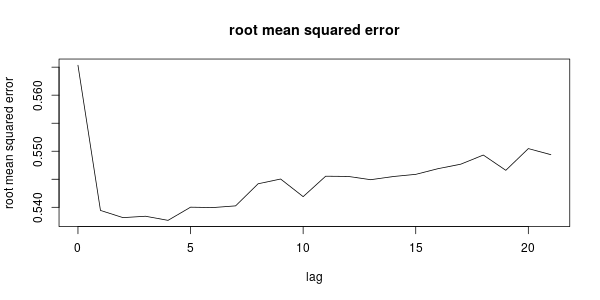
We note that environmental factors may not have an immediate effect on the number of recorded COVID-19 cases since there is 2-14 days of incubation period before the onset of symptoms and it takes another 2-7 days before a test result is available. To study whether there are lagging effects between the predictor and response variables, we fit a varying coefficient model with predictor-specific knots, for each time lag $\tau$, i.e., using data $y_{i}(t_{i,k}+\tau)$ and $x_{i,j}(t_{i,k})\ (j=1,\ldots,7)$, to fit model (8) similarly as in Fan & Zhang, (1999). Figure 4 shows the residual root mean squared error for each time lag. We find that the root mean squared error is the smallest with 4 days lag. Note that $y_{i}(t)$ represents the logarithm of the weekly average between day $t$ and $t+6$. This means the predictors at day $t$ are most predictive for infected numbers between day $t+4$ and $t+10$, which is consistent with the incubation period and test duration.

We consider the Boston housing price data from Harrison & Rubinfeld, (1978) with $n=506$ observations for the census districts of the Boston metropolitan area. The data is available in the R-package lmbench. Following (Wang et al.,, 2009; Hu & Xia,, 2012), we use medv (mediam value of owner-occupied homes in 1,000 USD) as the response, and lstat as the conditioner, which is defined as a linear combination of the proportion of adults with high school education or above and proportion of male workers classified as laborers. The predictors are: int (the intercept), crim (per capita crime rate by town), rm (average number of rooms per dwelling), ptratio (pupil-teacher ratio by town), nox (nitric oxides concentration parts per 10 million), tax (full-value property-tax rate per 10,000 USD), and age (proportion of owner-occupied units built prior to 1940). We transform the conditioner lstat so that its marginal distribution is $\rm{U}(0,1)$, and make a logarithm transformation of the response medv. For the predictors (except for intercept), we first transform them to the standard normal. Since some of the predictors are highly correlated with the conditioner, we further regress each predictor against the transformed lstat , and use the normalized residuals in the follow-up analysis.

We fit a predictor-specific varying coefficient linear model to predict the response with the residualized predictors using lstat as the conditioner. Figure 5 shows the fitted coefficients as a function of the conditioner, with the red lines showing the 95% confidence interval and the dashed lines being the x-axis. The confidence interval are computed conditioning on the selected knots for each predictor. The results show clear conditioner-varying effects of most predictors. The intercept appears to vary most significantly along with lstat, demonstrating that the the housing price is negatively and nearly linearly impacted by lstat. The coefficient for rm is in general positive, but trends towards insignificant as lstat increases. An interpretation is that houses with more rooms are generally more expensive, but its impact becomes insignificant in areas where lstat is large. The variable crim is highly correlated with lstat. After regressing out lstat, the residualized crim has an interesting fluctuation: varying from insignificant to positive and then to negative. We suspect that the positive impact of crim for certain areas may be due to a confounding effect with other unused variables such as the location’s convenience and attractiveness for tourists.

We also compare the predictive power of the simple linear model and the varying coefficient model by 10-fold cross validation. For the simple linear model, we include all the predictors used in the varying coefficient model as well as the conditioner lstat . The mean squared error (MSE) for the simple linear model is 23.52 while the MSE for the varying coefficient model is 20.51. When comparing the MSE, the observed and predicted responses are transformed back to the original scale. The results show that the varying coefficient model can better describe the relationship between the housing price and the predictors.

References

- Astrid et al., (2009) Astrid, J., Philippe, L., Benoit, B., & F, V. (2009). Pharmacokinetic parameters estimation using adaptive bayesian p-splines models. Pharm Stat, 8.
- Casas & Fernandez-Casal, (2019) Casas, I. & Fernandez-Casal, R. (2019). tvreg: Time-varying coefficient linear regression for single and multi-equations in r. SSRN.
- Chen et al., (2015) Chen, Y., Wang, Q., & Yao, W. (2015). Adaptive estimation for varying coefficient models. Journal of Multivariate Analysis, 137, 17–31.
- Fan & Zhang, (1999) Fan, J. & Zhang, W. (1999). Statistical estimation in varying coefficient models. The Annals of Statistics, 27(5), 1491 – 1518.
- Fan & Zhang, (2000) Fan, J. & Zhang, W. (2000). Simultaneous confidence bands and hypothesis testing in varying-coefficient models. Scandinavian Journal of Statistics, 27(4), 715–731.
- Finley & Banerjee, (2020) Finley, A. O. & Banerjee, S. (2020). Bayesian spatially varying coefficient models in the spbayes r package. Environmental Modelling & Software, 125, 104608.
- Harrison & Rubinfeld, (1978) Harrison, D. & Rubinfeld, D. L. (1978). Hedonic housing prices and the demand for clean air. Journal of environmental economics and management, 5(1), 81–102.
- Hastie & Tibshirani, (1993) Hastie, T. & Tibshirani, R. (1993). Varying-coefficient models. Journal of the Royal Statistical Society. Series B (Methodological), 55(4), 757–796.
- Hu et al., (2019) Hu, L., Huang, T., & You, J. (2019). Estimation and identification of a varying-coefficient additive model for locally stationary processes. Journal of the American Statistical Association, 114(527), 1191–1204.
- Hu & Xia, (2012) Hu, T. & Xia, Y. (2012). Adaptive semi-varying coefficient model selection. Statistica Sinica, (pp. 575–599).
- Huang & Shen, (2004) Huang, J. Z. & Shen, H. (2004). Functional coefficient regression models for non-linear time series: A polynomial spline approach. Scandinavian Journal of Statistics, 31(4), 515–534.
- Huang et al., (2002) Huang, J. Z., Wu, C. O., & Zhou, L. (2002). Varying-coefficient models and basis function approximations for the analysis of repeated measurements. Bimoetrika, 89(1), 111–128.
- Huang et al., (2004) Huang, J. Z., Wu, C. O., & Zhou, L. (2004). Polynomial spline estimation and inference for varying coefficient models with longitudinal data. Statistica Sinica, (pp. 763–788).
- Lin et al., (2019) Lin, H., Yang, B., Zhou, L., Yip, P. S., Chen, Y.-Y., & Liang, H. (2019). Global kernel estimator and test of varying-coefficient autoregressive model. Canadian Journal of Statistics, 47(3), 487–519.
- Notari, (2021) Notari, A. (2021). Temperature dependence of covid-19 transmission. Science of The Total Environment, 763, 144390.
- Schwarz et al., (1978) Schwarz, G. et al. (1978). Estimating the dimension of a model. The annals of statistics, 6(2), 461–464.
- Tang & Cheng, (2012) Tang, Q. & Cheng, L. (2012). Componentwise b-spline estimation for varying coefficient models with longitudinal data. Statistical Papers, 53, 629–652.
- Wang et al., (2009) Wang, H. J., Zhu, Z., & Zhou, J. (2009). Quantile regression in partially linear varying coefficient models. The Annals of Statistics, 37(6B), 3841–3866.
- Wang & Sun, (2019) Wang, W. & Sun, Y. (2019). Penalized local polynomial regression for spatial data. Biometrics, 75(4), 1179–1190.
- Wang et al., (2017) Wang, X., Jiang, B., & Liu, J. (2017). Generalized r-squared for detecting dependence. Biometrika, 104(1), 129–139.
- Wei et al., (2011) Wei, F., Huang, J., & Li, H. (2011). Variable selection and estimation in high-dimensional varying-coefficient models. Statistica Sinica, 21(4), 1515.
- Yuan & Lin, (2006) Yuan, M. & Lin, Y. (2006). Model selection and estimation in regression with grouped variables. Journal of the Royal Statistical Society: Series B (Statistical Methodology), 68(1), 49–67.
- Zhang & Wang, (2014) Zhang, X. & Wang, J.-L. (2014). Varying-coefficient additive models for functional data. Biometrika, 102(1), 15–32.
- Zou, (2006) Zou, H. (2006). The adaptive lasso and its oracle properties. Journal of the American statistical association, 101(476), 1418–1429.