Variational setting for cracked beams and shallow arches

Detection of cracks is an important engineering problem. It requires a rigorous mathematical framework for modeling the motion of cracked beams and shallow arches. The main goal of this paper is to develop a variational setting for such a framework. We also present an elegant and efficient method (a modification of the Shifrin’s method) for the computation of the eigenvalues and the eigenfunctions for the cracked elements.

For a theory of cracked Bernoulli-Euler beams see [5]. A significant effort has been directed at the vibration analysis of cracked beams. Representation of a crack by a rotational spring has been proven to be accurate, and it is often used, see [2, 3] and the extensive bibliography there. Determination of the beam natural frequencies is discussed in [11, 13, 14]. S. Caddemi and his colleagues have further developed the theory using energy functions in [3]. However, no full variational setting has been presented so far, making it difficult to study evolution problems. As we have already mentioned, our work closes a gap in this development.

The theory of uniform beams and shallow arches is well developed. An early exposition can be found in [1]. More general models in the multidimensional setting, and a literature survey are presented in [6]. A review for vibrating beams is given in [10]. Motion of uniform arches and a related parameter estimation problem are studied in [8]. These results are extended to point loads in [7]. The existence of a compact, uniform attractor is established in [9].

The transverse motion of a beam or an arch is described by the function $y(x,t),\,x\in[0,\pi],\,t\geq 0$, which represents the deformation of the beam/arch measured from the $x$-axis. For definiteness, the boundary conditions are of the hinged type

Other types of boundary conditions, can be treated similarly.

Crack modeling is considered in Section 2. Suppose that there are $m$ cracks located at $0<x_{1}<x_{2}<\dots<x_{m}<\pi$. A crack at $x=x_{i}$ is represented by a rotational spring with the flexibility $\theta_{i}$, $i=1,\dots,m$. This is expressed as

In Section 3 we introduce special Hilbert spaces $V$ and $H$ satisfying

with continuous and dense embeddings. These spaces are broad enough to contain continuous functions with discontinuous derivatives at the joint points.

Section 4 contains our main result. We introduce the operator $\mathcal{A}:V\to V^{\prime}$, by

for any $u,v\in V$, where $J[u^{\prime}](x)=u^{\prime}(x^{+})-u^{\prime}(x^{-})$.

Then we show that the solution $u$ of the equation $\mathcal{A}u=f$ in $H$ satisfies the joint conditions, including (1.2). Thus the operator $\mathcal{A}$ ”absorbs” the boundary conditions, as expected of the weak formulation of the steady state problem.

This result allows us to prove the existence of the eigenvalues and the eigenfunctions of $\mathcal{A}$. An efficient Modified Shifrin’s Method for their computation is presented in Section 5.

The results in this paper form the basis for a comprehensive study of dynamic behavior of cracked beams and arches. It will be presented elsewhere.

A crack is a disruption in the material, that has a negligible extent in the direction of the beam/arch axis, but of a non-negligible depth. It is fully described by its position along the axis, and the crack depth ratio $\hat{\mu}$, as shown in Figure 1.

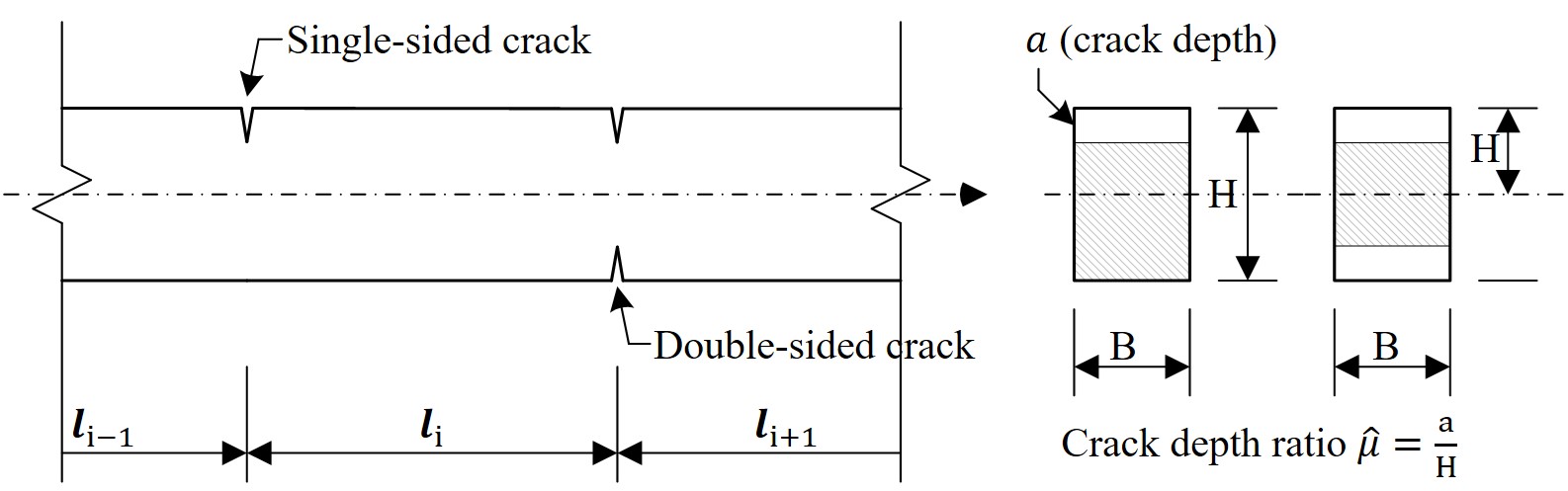
According to [4], a crack is modeled by a massless rotational spring. The spring flexibility $\theta=\theta(\hat{\mu})$ depends on the crack depth ratio $\hat{\mu}$, and on whether the crack is one-sided or two-sided, open or closed, and so on. The flexibility $\theta$ is equal to $0$ if there is no crack, and it increases with the crack depth. Explicit expressions for the functions $\theta(\hat{\mu})$ are provided in Section 5.

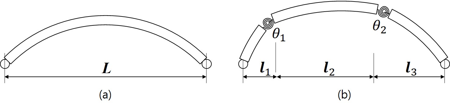
Suppose that there are $m$ cracks along the length of the arch, located at $0<x_{1}<\dots<x_{m}<\pi$. For convenience, we denote $x_{0}=0$, and $x_{m+1}=\pi$. Consequently, the cracked arch is modeled as a collection of $m+1$ uniform arches over the intervals $l_{i}=(x_{i-1},x_{i}),\,i=1,\dots,m+1$, as shown in Figure 2(b).

We consider only the transverse motion of the arch, so its position can be described by the function $y=y(x,t)$, $0\leq x\leq\pi$, $t\geq 0$. The boundary conditions at the cracks enforce the continuity of the displacement field $y$, the bending moment $y^{\prime\prime}$, and the shear force $y^{\prime\prime\prime}$. Condition $y^{\prime}(x_{i}^{+},t)-y^{\prime}(x_{i}^{-},t)=\theta_{i}y^{\prime\prime}(x_{i}^{+},t)$ expresses the discontinuity of the arch slope at the $i$-th crack, where $\theta_{i}=\theta(\hat{\mu}_{i})$, see Figure 2(b).

To simplify the statement of the boundary conditions at the cracks, we introduce the notion of the jump $J[u](x)$ of a function $u=u(x)$ at any $x\in(0,\pi)$, as follows

With this notation the conditions at the cracks (joint conditions) are

and

where $\theta_{i}=\theta(\hat{\mu}_{i})$, $i=1,2,\dots,m$ and $t\geq 0$. Note that $y^{\prime\prime}(x_{i}^{+},t)=y^{\prime\prime}(x_{i}^{-},t)$ by (2.2).

We introduce Hilbert spaces $H$ and $V$ suitable for working with cracked elements. Suppose that an arch has $m$ cracks at the joint points $0<x_{1}<\dots<x_{m}<\pi$. This partition of the interval $[0,\pi]$ is associated with $m+1$ subintervals $l_{i}=(x_{i-1},x_{i}),\,m=1,\dots,m+1$.

Let $H$ be the Hilbert space

Let the inner product and the norm in $L^{2}(l_{i})$ be denoted by $(\cdot,\cdot)_{i}$ and $|\cdot|_{i}$ correspondingly. The inner product and the norm in $H$ are defined by

Consider the Sobolev space $H^{2}(a,b)$ on a bounded interval $(a,b)\subset{\mathbb{R}}$, and let $u\in H^{2}(a,b)$. Then $u,u^{\prime}$ are continuous functions on $[a,b]$, up to a set of measure zero, and $u^{\prime\prime}\in L^{2}(a,b)$. Therefore, for such $u$, we will always assume that $u,u^{\prime}\in C[a,b]$.

Define the linear space

We interpret $u\in V$ as a continuous function on $[0,\pi]$, such that $u(0)=u(\pi)=0$, with $u^{\prime}\in L^{2}(0,\pi)$, i.e. $u\in H_{0}^{1}(0,\pi)$. Furthermore, $u|_{l_{i}}\in H^{2}(l_{i})$, and $u^{\prime}|_{l_{i}}\in C[x_{i-1},x_{i}]$ for $i=1,2,\dots,m+1$.

Define the inner product on $V$ by

where $(u^{\prime\prime},v^{\prime\prime})_{i}=\int_{l_{i}}u^{\prime\prime}(x)v^{\prime\prime}(x)\,dx$.

It is clear that $((\cdot,\cdot))_{V}$ is a symmetric, bilinear form on $V$. To see that $((u,u))_{V}=0$ implies $u=0$, notice that any function $u$ with $((u,u))_{V}=0$ is piecewise linear and continuous on $[0,\pi]$. Furthermore, $J[u^{\prime}](x_{i})=0$ for any $i=1,2,\dots,m$. Therefore $u^{\prime}$ is continuous on $[0,\pi]$. In fact, it is a constant there, since $u^{\prime\prime}=0$ a.e. on $[0,\pi]$. Thus $u$ is a linear function on $[0,\pi]$ satisfying the zero boundary conditions at the ends of the interval. Therefore $u=0$ on $[0,\pi]$, and $((\cdot,\cdot))_{V}$ is a well-defined inner product on $V$. The corresponding norm in $V$ is

where $|\cdot|_{i}$ is the norm in $L^{2}(l_{i})$. We will show in Lemma 3.2 that $V$ is a Hilbert space.

Let $u\in V$. We define the derivatives of $u$ component-wise in the spaces $H^{2}(l_{i})$, that is $u^{\prime}(x)=(u|_{l_{i}})^{\prime}(x),u^{\prime\prime}(x)=(u|_{l_{i}})^{\prime\prime}(x)$, and so on, for $x\in l_{i}$, $i=1,\dots,m+1$. For definiteness, we will assume that the derivative $u^{\prime}$ is continuous from the right on $[0,\pi]$.

Some useful properties of functions in $V$ are established in the following lemma.

Lemma 3.3 allows us to define the Gelfand triple $V\subset H\subset V^{\prime}$, with the dense embeddings. Furthermore, the embedding $V\subset H$ is compact. The pairing $\langle\cdot,\cdot\rangle_{V}$ between $V$ and $V^{\prime}$ extending the inner product in $H$. This means that given $f\in H=H^{\prime}\subset V^{\prime}$, and $v\in V$, we have $\langle f,v\rangle_{V}=(f,v)_{H}$.

We introduce the operator $\mathcal{A}:V\to V^{\prime}$ that ”absorbs” the junction boundary conditions. This operator is central to the variational setting of problems for cracked beams and arches. The existence of its eigenvalues and the eigenfunctions is established as well.

See Section 2 for the setup for the junction (crack) points $x_{i}$, and the flexibilities $\theta_{i}$. Recall, that a linear operator $A:V\to V^{\prime}$ is called coercive, if there exists $c>0$, such that $\langle Au,u\rangle\geq c\|u\|^{2}_{V}$ for any $u\in V$.

As was mentioned in Section 2, functions $u=u(x)$ modeling an arch with cracks are expected to satisfy certain boundary conditions. For convenience, we restate them here:

and

for $i=1,\dots,m$.

The next theorem is the main result of this paper.

Remark. The fact that $u^{\prime\prime\prime\prime}=f$ a.e. on $(0,\pi)$ in Theorem 4.3 does not imply that $u\in H^{4}(0,\pi)$. This is similar to the fact that the strong derivative $p^{\prime}$ of a step function $p$ on $(0,\pi)$ is zero a.e. on $(0,\pi)$. However, $p\not\in H^{1}(0,\pi)$.

Finally in this section we discuss the eigenvalues and the eigenfunctions of the operator $\mathcal{A}$. It was shown in Lemma 4.2 that $\mathcal{A}$ is a continuous, linear, symmetric, and coercive operator from $V$ onto $V^{\prime}$. Following [15, Section 2.2.1], $\mathcal{A}$ can also be considered as an unbounded operator in $H$. By Lemma 3.3, the embedding $V\subset H$ is compact. Therefore the standard spectral theory for Sturm-Liouville boundary value problems is applicable. The eigenfunctions belong to $H$. Therefore, by Theorem 4.3, they are in the domain $D(\mathcal{A})\subset V$, thus continuous on $[0,\pi]$, and satisfy conditions (4.2)–(4.3).

We summarize these results in the following lemma.

Algorithms for a computational determination of the eigenvalues and the eigenfunctions of $\mathcal{A}$ are discussed in Section 5.

Remark. If the arch is uniform, i.e. it has no cracks, then the results presented in this section are simplified. Specifically, the spaces $V,H$, and the operator $\mathcal{A}$ take the following forms

for any $u,v\in V$. See [8] for an investigation of this case.

In this section we present the Modified Shifrin’s method for the computation of the eigenfunctions $\varphi_{k},\,k\geq 1$ and the corresponding eigenvalues $\lambda^{4}_{k}$, of the operator $\mathcal{A}$. The existence of the eigenvalues and the eigenfunctions has been established in Lemma 4.4.

Transition matrices method. This is a common method for the determination of the eigenfunctions and the eigenvalues, so we just briefly mention it for completeness, see [11] for details.

The general solution of the equation $w^{\prime\prime\prime\prime}=\lambda^{4}w$ on $l_{i}=(x_{i-1},x_{i})$, for $i=1,\dots,m+1$ is

Let vector $\vec{A}_{i}=[A_{i},B_{i},C_{i},D_{i}]^{T}$ be composed of the coefficients of the expansion in (5.1), on interval $l_{i}$.

Suppose that vector $\vec{A}_{1}$ is known. Then it defines function $w_{1}^{\lambda}$ on $l_{1}$, and the boundary conditions for $w_{1}^{\lambda}$ at $x_{1}^{-}$. The junction conditions (4.2)–(4.3) define the boundary conditions for $w_{2}^{\lambda}$ at $x_{1}^{+}$. Then the initial value problem $(w_{2}^{\lambda})^{\prime\prime\prime\prime}=\lambda^{4}w_{2}^{\lambda}$ on $l_{2}=(x_{1},x_{2})$, uniquely defines the expansion coefficients $\vec{A}_{2}$ on $l_{2}$. It is readily seen that the transformation from $\vec{A}_{1}$ to $\vec{A}_{2}$ is linear, and it is given by a $4\times 4$ matrix $T^{(1)}$, i.e. $\vec{A}_{2}=T^{(1)}\vec{A}_{1}$.

Extending this process to all the subintervals $l_{i},i=1,\dots,m+1$, we get

Note that all the matrices $T^{(i)}$ are $\lambda$-dependent in a non-linear way.

To satisfy the hinged boundary conditions at $x=0$, we require $\vec{A}_{1}=[A_{1},0,C_{1},0]^{T}$.

References

- [1] J.M. Ball, Initial-boundary value problems for an extensible beam, J. Math. Anal. Appl, 42 (1973) 61-90.
- [2] S. Caddemi and I. Calio, Exact closed-form solution for the vibration modes of the Euler–Bernoulli beam with multiple open cracks, Journal of Sound and Vibration, 327(3), 1973, 473 - 489.
- [3] S. Caddemi and A. Morassi, Multi-cracked Euler-Bernoulli beams: Mathematical modeling and exact solutions, International Journal of Solids and Structures, 50(6), 2013, 944-956.
- [4] M.N. Cerri and G.C. Ruta, Detection of localised damage in plane circular arches by frequency data, Journal of Sound and Vibration, 270(1), 2004, 39-59.
- [5] S. Christides and A.D.S. Barr, One-dimensional theory of cracked Bernoulli-Euler beams, International Journal of Mechanical Sciences, 26(11), 1984, 639-648
- [6] E. Emmrich and M. Thalhammer, A class of integro-differential equations incorporating nonlinear and nonlocal damping with applications in nonlinear elastodynamics: Existence via time discretization, Nonlinearity, 24(9), 2011, 2523-2546.
- [7] S. Gutman and J. Ha, Shallow arches with weak and strong damping, Journal of the Korean Mathematical Society 54(5), 2017, 945-966.
- [8] S. Gutman and J. Ha and S. Lee, Parameter identification for weakly damped shallow arches, Journal of Mathematical Analysis and Applications, 403(1), 2013, 297-313.
- [9] S. Gutman and J. Ha, Uniform attractor of shallow arch motion under moving points load, Journal of Mathematical Analysis and Applications, 464(1), 2018, 557-579.
- [10] S. M. Han and H. Benaroya and T. Wei, Dynamics of transversely vibrating beams using four engineering theories, Journal of Sound and Vibration, 225(5), 1999, 935-988.
- [11] H.P. Lin and S.C. Chang and J.D. Wu, Beam vibrations with an arbitrary number of cracks, Journal of Sound and Vibration, 258(5), 2002, 987-999.
- [12] J.L. Lions and E. Magenes, Nonhomogeneous Boundary Value Problems and Applications, vol 1, 1972, Springer-Verlag, New York.
- [13] W.M. Ostachowicz and M. Krawczuk, Analysis of the effect of cracks on the natural frequencies of a cantilever beam, Journal of Sound and Vibration, 150(2), 1991, 191-201.
- [14] E.I. Shifrin and R. Ruotolo, Natural frequencies of a beam with an arbitrary number of cracks, Journal of Sound and Vibration, 222(3), 1999, 409-423.
- [15] R. Temam, Infinite-Dimensional Dynamical Systems in Mechanics and Physics, Applied Mathematical Sciences, 1997, Springer, New York.