Variational Leakage: The Role of
Information Complexity in Privacy Leakage

Sensitive information sharing is a challenging problem in information systems. It is often handled by obfuscating the available information before sharing it with other parties. In (Makhdoumi et al., 2014), this problem has been formalized as the privacy funnel (PF) in an information theoretic framework. Given two correlated random variables $\mathbf{S}$ and $\mathbf{X}$ with a joint distribution $P_{\mathbf{S},\mathbf{X}}\,$, where $\mathbf{X}$ represents the available information and $\mathbf{S}$ the private latent variable, the goal of the PF model is to find a representation $\mathbf{Z}$ of $\mathbf{X}$ using a stochastic mapping $P_{\mathbf{Z}\mid\mathbf{X}}$ such that: (i) $\mathbf{S}\hbox{$\--$}\kern-1.5pt\hbox{$\circ$}\kern-1.5pt\hbox{$\--$}\mathbf{X}\hbox{$\--$}\kern-1.5pt\hbox{$\circ$}\kern-1.5pt\hbox{$\--$}\mathbf{Z}$ form a Markov chain; and (ii) representation $\mathbf{Z}$ is maximally informative about the useful data $\mathbf{X}$ (maximizing Shannon’s mutual information (MI) $\mathrm{I}\left(\mathbf{X};\mathbf{Z}\right)$) while being minimally informative about the sensitive data $\mathbf{S}$ (minimizing $\mathrm{I}\left(\mathbf{S};\mathbf{Z}\right)$). There have been many extensions of this model in the recent literature, e.g., (Makhdoumi et al., 2014; P. Calmon et al., 2015; Basciftci et al., 2016; Sreekumar and Gündüz, 2019; Hsu et al., 2019; Rassouli et al., 2019; Rassouli and Gündüz, 2019; Razeghi et al., 2020; Rassouli and Gündüz, 2021).

In this paper, we will consider a delicate generalization of the PF model considered in (Basciftci et al., 2016; Rassouli and Gündüz, 2021), where the goal of the system designer is not to reveal the data that has available but another correlated utility variable. In particular, we assume that the data owner/user acquires some utility from the service provider based on the amount of information disclosed about a utility random variable $\mathbf{U}$ correlated with $\mathbf{X}$, measured by $\mathrm{I}\!\left(\mathbf{U};\mathbf{Z}\right)$. Therefore, considering Markov chain $\left(\mathbf{U},\mathbf{S}\right)\hbox{$\--$}\kern-1.5pt\hbox{$\circ$}\kern-1.5pt\hbox{$\--$}\mathbf{X}\hbox{$\--$}\kern-1.5pt\hbox{$\circ$}\kern-1.5pt\hbox{$\--$}\mathbf{Z}$, the data owner’s aim is to share a representation $\mathbf{Z}$ of observed data $\mathbf{X}$, through a stochastic mapping $P_{\mathbf{Z}\mid\mathbf{X}}$, while preserving information about utility attribute $\mathbf{U}$ and obfuscate information about sensitive attribute $\mathbf{S}$ (see Fig. 1).

The implicit assumption in the PF model presented above and the related generative adversarial privacy framework (Huang et al., 2017; Tripathy et al., 2019) is to have pre-defined interests in the game between the ‘defender’ (data owner/user) and the ‘adversary’; that is, the data owner knows in advance what feature/ variable of the underlying data the adversary is interested in. Accordingly, the data release mechanism can be optimized/ tuned to minimize any inference the adversary can make about this specific random variable. However, this assumption is violated in most real-world scenarios. The attribute that the defender may assume as sensitive may not be the attribute of interest for the inferential adversary. As an example, for a given utility task at hand, the defender may try to restrict inference on gender recognition while the adversary is interested in inferring an individual’s identity or facial emotion. Inspired by (Issa et al., 2019), and in contrast to the above setups, we consider the scenario in which the adversary is curious about an attribute that is unknown to the system designer.

In particular, we argue that the information complexity of the representation measured by MI $\mathrm{I}\!\left(\mathbf{X};\mathbf{Z}\right)$ can also limit the information leakage about the unknown sensitive variable. In this paper, obtaining the parameterized variational approximation of information quantities, we investigate the core idea of (Issa et al., 2019) in the supervised representation learning setup.

Given the observed data $\mathbf{X}$, the data owner wishes to release a representation $\mathbf{Z}$ for a utility task $\mathbf{U}$. Our aim is to investigate the potential statistical inference about a sensitive random attribute $\mathbf{S}$ from the released representation $\mathbf{Z}$. The sensitive attribute $\mathbf{S}$ is possibly also correlated with $\mathbf{U}$ and $\mathbf{X}$.

The objective is to obtain a stochastic map $P_{\mathbf{Z}\mid\mathbf{X}}:\!\mathcal{X}\rightarrow\mathcal{Z}$ such that $P_{\mathbf{U}\mid\mathbf{Z}}\!\approx\!P_{\mathbf{U}\mid\mathbf{X}},\forall\,\mathbf{Z}\!\in\!\mathcal{Z},\forall\,\mathbf{U}\!\in\!\mathcal{U},\forall\,\mathbf{X}\!\in\!\mathcal{X}$. This means that the posterior distribution of the utility attribute $\mathbf{U}$ is similar when conditioned on the released representation $\mathbf{Z}$ or on the original data $\mathbf{X}$. Under logarithmic loss, one can measure the utility by Shannon’s MI (Makhdoumi et al., 2014; Tishby et al., 2000; Razeghi et al., 2020). The logarithmic loss function has been widely used in learning theory (Cesa-Bianchi and Lugosi, 2006), image processing (Andre et al., 2006), information bottleneck (Harremoës and Tishby, 2007), multi-terminal source coding (Courtade and Wesel, 2011), and PF (Makhdoumi et al., 2014).

Threat Model: We make minimal assumptions about the adversary’s goal, which can model a large family of potential adversaries. In particular, we have the following assumptions:

• •

  The distribution $P_{\mathbf{S}\mid\mathbf{X}}$ is unknown to the data user/owner. We only restrict attribute $\mathbf{S}$ to be discrete, which captures most scenarios of interest, e.g., a facial attribute, an identity, a political preference.

• •

  The adversary observes released representation $\mathbf{Z}$ and the Markov chain $(\mathbf{U},\mathbf{S})\hbox{$\--$}\kern-1.5pt\hbox{$\circ$}\kern-1.5pt\hbox{$\--$}\mathbf{X}\hbox{$\--$}\kern-1.5pt\hbox{$\circ$}\kern-1.5pt\hbox{$\--$}\mathbf{Z}$ holds.

• •

  We assume the adversary knows the mapping $P_{\mathbf{Z}\mid\mathbf{X}}$ designed by the data owner, i.e., the data release mechanism is public. Furthermore, the adversary may have access to a collection of the original dataset with the corresponding labels $\mathbf{S}$.

Suppose that the sensitive attribute $\mathbf{S}\!\in\!\mathcal{S}$ has a uniform distribution over a discrete set $\mathcal{S}$, where $|\mathcal{S}|\!=\!2^{L}\!<\!\infty$. If $\mathrm{I}(\mathbf{S};\mathbf{Z})\geq L-\epsilon$, then equivalently $\mathrm{H}(\mathbf{S}\!\mid\!\mathbf{Z})\leq\epsilon$. Also note that due to the Markov chain $\mathbf{S}\hbox{$\--$}\kern-1.5pt\hbox{$\circ$}\kern-1.5pt\hbox{$\--$}\mathbf{X}\hbox{$\--$}\kern-1.5pt\hbox{$\circ$}\kern-1.5pt\hbox{$\--$}\mathbf{Z}$, we have $\mathrm{I}(\mathbf{S};\mathbf{Z})=\mathrm{I}(\mathbf{X};\mathbf{Z})-\mathrm{I}(\mathbf{X};\mathbf{Z}\mid\mathbf{S})$. When $\mathbf{S}$ is not known a priori, the data owner has no control over $\mathrm{I}(\mathbf{X};\mathbf{Z}\!\mid\!\mathbf{S})$. On the other hand, $\mathrm{I}(\mathbf{X};\mathbf{Z})$ can be interpreted as the information complexity of the released representation, which plays a critical role in controlling the information leakage $\mathrm{I}(\mathbf{S};\mathbf{Z})$. Note also that a statistic $\mathbf{Z}\!=\!f\!\left(\mathbf{X}\right)$ induces a partition on the sample space $\mathcal{X}$, where $\mathbf{Z}$ is sufficient statistic for $\mathbf{U}$ if and only if the assigned samples in each partition do not depend on $\mathbf{U}$. Hence, intuitively, a larger $|\mathcal{U}|$ induces finer partitions on $\mathcal{X}$, which could potentially lead to more leakage about the unknown random function $\mathbf{S}$ of $\mathbf{X}$. This is the core concept of the notion of variational leakage, which we shortly address in our experiments.

Since the data owner does not know the particular sensitive variable of interest to the adversary, we argue that it instead aims to design $P_{\mathbf{Z}\mid\mathbf{X}}$ with the minimum (information) complexity and minimum utility loss. With the introduction of a Lagrange multiplier $\beta\!\in\!\left[0,1\right]$, we can formulate the objective of the data owner by maximizing the associated Lagrangian functional:

This is the well-known information bottleneck (IB) principle (Tishby et al., 2000), which formulates the problem of extracting, in the most succinct way, the relevant information from random variable $\mathbf{X}$ about the random variable of interest $\mathbf{U}$. Given two correlated random variables $\mathbf{U}$ and $\mathbf{X}$ with joint distribution $P_{\mathbf{U,X}}$, the goal is to find a representation $\mathbf{Z}$ of $\mathbf{X}$ using a stochastic mapping $P_{\mathbf{Z}\mid\mathbf{X}}$ such that: (i) $\mathbf{U}\hbox{$\--$}\kern-1.5pt\hbox{$\circ$}\kern-1.5pt\hbox{$\--$}\mathbf{X}\hbox{$\--$}\kern-1.5pt\hbox{$\circ$}\kern-1.5pt\hbox{$\--$}\mathbf{Z}$, and (ii) $\mathbf{Z}$ is maximally informative about $\mathbf{U}$ (maximizing $\mathrm{I}\left(\mathbf{U};\mathbf{Z}\right)$) and minimally informative about $\mathbf{X}$ (minimizing $\mathrm{I}\left(\mathbf{X};\mathbf{Z}\right)$).

Note that in the PF model, $\mathrm{I}\left(\mathbf{X};\mathbf{Z}\right)$ measures the useful information, which is of the designer’s interest, while in the IB model, $\mathrm{I}\left(\mathbf{U};\mathbf{Z}\right)$ measures the useful information. Hence, $\mathrm{I}\left(\mathbf{X};\mathbf{Z}\mid\mathbf{S}\right)$ in PF quantifies the residual information, while $\mathrm{I}\left(\mathbf{X};\mathbf{Z}\mid\mathbf{U}\right)$ in IB quantifies the redundant information.

In the sequel, we provide the parameterized variational approximation of information quantities, and then study the impact of the information complexity $\mathrm{I}\left(\mathbf{X};\mathbf{Z}\right)$ on the information leakage for an unknown sensitive variable.

System Designer. Given independent and identically distributed (i.i.d.) training samples $\{\left(\mathbf{u}_{n},\mathbf{x}_{n}\right)\}_{n=1}^{N}$ $\subseteq\mathcal{U}\times\mathcal{X}$, and using stochastic gradient descent (SGD)-type approach, DNNs $f_{\bm{\phi}}$, $g_{\bm{\theta}}$, $D_{\bm{\eta}}$, and $D_{\bm{\omega}}$ are trained together to maximize a Monte-Carlo approximation of the deep variational IB functional over parameters $\bm{\phi}$, $\bm{\theta}$, $\bm{\eta}$, and $\bm{\omega}$ (Fig. 2). Backpropagation through random samples from the posterior distribution $P_{\bm{\phi}}(\mathbf{Z}\!\!\mid\!\!\mathbf{X})$is required in our framework, which is a challenge since backpropagation cannot flow via random nodes; to overcome this hurdle, we apply the reparameterization approach (Kingma and Welling, 2014)).

The inferred posterior distribution is typically assumed to be a multi-variate Gaussian with a diagonal co-variance, i.e., $P_{\bm{\phi}}(\mathbf{Z}\!\mid\!\mathbf{x})=\mathcal{N}\big{(}\bm{\mu}_{\bm{\phi}}(\mathbf{x}),$ $\mathsf{diag}(\bm{\sigma}_{\bm{\phi}}(\mathbf{x}))\big{)}$. Suppose $\mathcal{Z}=\mathbb{R}^{d}$. We first sample a random variable $\bm{\mathcal{E}}$ i.i.d. from $\mathcal{N}\!\left(\bm{0},\mathbf{I}_{d}\right)$, then given data sample $\mathbf{x}\in\mathcal{X}$, we generate the sample $\mathbf{z}=\bm{\mu}_{\bm{\phi}}(\mathbf{x})+\bm{\sigma}_{\bm{\phi}}(\mathbf{x})\odot\bm{\varepsilon}$, where $\odot$ is the element-wise (Hadamard) product. The latent space prior distribution is typically considered as a fixed $d$-dimensional standard isotropic multi-variate Gaussian, i.e., $Q_{\mathbf{Z}}=\mathcal{N}\!\left(\bm{0},\mathbf{I}_{d}\right)$. For this simple choice, the information complexity upper bound

The $\mathrm{KL}$-divergences in (3) and (2.1) can be estimated using the density-ratio trick (Nguyen et al., 2010; Sugiyama et al., 2012), utilized in the GAN framework to directly match the data and generated model distributions. The trick is to express two distributions as conditional distributions, conditioned on a label $C\in\{0,1\}$, and reduce the task to binary classification. The key point is that we can estimate the KL-divergence by estimating the ratio of two distributions without modeling each distribution explicitly.

Consider $\mathrm{D}_{\mathrm{KL}}\!\left(P_{\bm{\phi}}(\mathbf{Z})\,\|\,Q_{\mathbf{Z}}\right)=\mathbb{E}_{P_{\bm{\phi}}(\mathbf{Z})}[\log\frac{P_{\bm{\phi}}(\mathbf{Z})}{Q_{\mathbf{Z}}}]$. We now define $\rho_{\mathbf{Z}}(\mathbf{z}\!\mid\!c)$ as $\rho_{\mathbf{Z}}(\mathbf{z}\!\mid\!c\!=\!1)\!=\!P_{\bm{\phi}}(\mathbf{Z})$, $\rho_{\mathbf{Z}}(\mathbf{z}\!\mid\!c\!=\!0)=Q_{\mathbf{Z}}$. Suppose that a perfect binary classifier (discriminator) $D_{\bm{\eta}}(\mathbf{z})$, with parameters $\bm{\eta}$, is trained to associate the label $c=1$ to samples from distribution $P_{\bm{\phi}}(\mathbf{Z})$ and the label $c=0$ to samples from $Q_{\mathbf{Z}}$. Using the Bayes’ rule and assuming that the marginal class probabilities are equal, i.e., $\rho(c=1)=\rho(c=0)$, the density ratio can be expressed as:

Therefore, given a trained discriminator $D_{\bm{\eta}}(\mathbf{z})$ and $M$ i.i.d. samples $\{\mathbf{z}_{m}\}_{m=1}^{M}$ from $P_{\bm{\phi}}(\mathbf{Z})$, we estimate $\mathrm{D}_{\mathrm{KL}}\!\left(P_{\bm{\phi}}(\mathbf{Z})\,\|\,Q_{\mathbf{Z}}\right)$ as:

Our model is trained using alternating block coordinate descend across five steps (See Algorithm 1).

Inferential Adversary: Given the publicly-known encoder $\bm{\phi}$ and $K$ i.i.d. samples $\{(\mathbf{s}_{k},\mathbf{z}_{k})\}_{k=1}^{K}\!\subseteq\mathcal{S}\times\mathcal{Z}$, the adversary trains an inference network $\bm{\xi}$ to minimize $\mathrm{H}_{\bm{\xi}}(\mathbf{S}\!\mid\!\mathbf{Z})$.

In this section, we show the impact of the following factors on the amount of leakage: (i) information complexity regularizer weight $\beta\!\in\!(0,1]$, (ii) released representation dimension $d_{\mathrm{z}}$, (iii) cardinalities of the known utility and unknown sensitive attribute sets, (iv) correlation between the utility and sensitive attributes, and (v) potential bias in a sensitive attribute of adversary’s interest. We conduct experiments on the Colored-MNIST and large-scale CelebA datasets. The Colored-MNIST¹¹1Several papers have employed Colored-MNIST dataset; However, they are not unique, and researchers synthesized different versions based on their application. The innovative concept behind our version was influenced from the one used in (Rodríguez-Gálvez et al., 2020). is our modified version of MNIST (LeCun and Cortes, 2010), which is a collection of $70,000$ colored digits of size $28\times 28$. The digits are randomly colored with red, green, or blue based on two distributions, as explained in the caption of Fig. 4. The CelebA (Liu et al., 2015) dataset contains $202,599$ images of size $218\times 178$. We used TensorFlow $2.4.1$ (Abadi et al., 2016) with Integrated Keras API. The method details and network architectures are provided in Appendix. A and Appendix B.

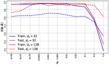
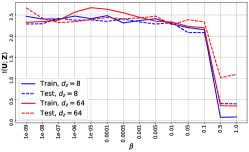
The first and second rows of Fig. 3 and Fig. 4 depict the trade-off among (i) information complexity, (ii) service provider’s accuracy on utility attribute $\mathbf{U}$, and (iii) adversary’s accuracy on attribute $\mathbf{S}$. The third row depicts the amount of information revealed about $\mathbf{S}$, i.e., $\mathrm{I}(\mathbf{S};\mathbf{Z})$, for the scenarios considered in the first and second rows, which are estimated using MINE (Belghazi et al., 2018). The fourth row depicts the amount of released information about the utility attribute $\mathbf{U}$, i.e., $\mathrm{I}(\mathbf{U};\mathbf{Z})$, corresponding to the considered scenarios in the first and second rows, also estimated using MINE. We consider different portions of the datasets available for training adversary’s network, denoted by the ‘data ratio’.

The experiments on CelebA consider the scenarios in which the attributes $\mathbf{U}$ and $\mathbf{S}$ are correlated, while $|\mathcal{U}|=|\mathcal{S}|=2$. We provide utility accuracy curves for (i) training set, (ii) validation set, and (iii) test set. As we have argued, there is a direct relationship between information complexity and intrinsic information leakage. Note that, as $\beta$ increases, the information complexity is reduced, and we observe that this also results in a reduction in the information leakage. We also see that the leakage is further reduced when the dimension of the released representation $\mathbf{Z}$, i.e., $d_{\mathrm{z}}$, is reduced. This forces the data owner to obtain a more succinct representation of the utility variable, removing any extra information.

In the Colored-MNIST experiments, provided that the model eliminates all the redundant information $\mathrm{I}(\mathbf{X};\mathbf{Z}\!\mid\!\mathbf{U})$ and leaves only the information about $\mathbf{U}$, we expect the adversary’s performance to be close to ‘random guessing’ since the digit color is independent of its value. We investigate the impact of the cardinality of sets $|\mathcal{U}|$ and $|\mathcal{S}|$, as well as possible biases in the distribution of $\mathbf{S}$. The results show that it is possible to reach the same level of accuracy on the utility attribute $\mathbf{U}$, while reducing the intrinsic leakage by increasing the regularizer weight $\beta$, or equivalently, by reducing the information complexity $\mathrm{I}_{\bm{\phi}}(\mathbf{X};\mathbf{Z})$. An interesting possible scenario is to consider correlated attributes $\mathbf{U}$ and $\mathbf{S}$ with different cardinality sets $\mathcal{U}$ and $\mathcal{S}$. For instance, utility task $\mathbf{U}$ is personal identification, while the adversary’s interest $\mathbf{S}$ is gender recognition.

We studied the variational leakage to address the amount of potential privacy leakage in a supervised representation learning setup. In contrast to the PF and generative adversarial privacy models, we consider the setup in which the adversary’s interest is not known a priori to the data owner. We study the role of information complexity in information leakage about an attribute of an adversary interest. This was addressed by approximating the information quantities using DNNs and experimentally evaluating the model on large-scale image databases. The proposed notion of variational leakage relates the amount of leakage to the minimal sufficient statistics.

References

- (1)
- Abadi et al. (2016) Martín Abadi et al. 2016. Tensorflow: A system for large-scale machine learning. In USENIX Symp. on Operating Sys. Design and Impl. (OSDI). 265–283.
- Andre et al. (2006) Thomas Andre, Marc Antonini, Michel Barlaud, and Robert M Gray. 2006. Entropy-based distortion measure for image coding. In 2006 International Conference on Image Processing. IEEE, 1157–1160.
- Basciftci et al. (2016) Yuksel Ozan Basciftci, Ye Wang, and Prakash Ishwar. 2016. On privacy-utility tradeoffs for constrained data release mechanisms. In 2016 Information Theory and Applications Workshop (ITA). IEEE, 1–6.
- Bauer and Mnih (2019) Matthias Bauer and Andriy Mnih. 2019. Resampled priors for variational autoencoders. In The 22nd International Conference on Artificial Intelligence and Statistics. 66–75.
- Belghazi et al. (2018) Mohamed Ishmael Belghazi, Aristide Baratin, Sai Rajeshwar, Sherjil Ozair, Yoshua Bengio, Aaron Courville, and Devon Hjelm. 2018. Mutual information neural estimation. In International Conference on Machine Learning. 531–540.
- Cesa-Bianchi and Lugosi (2006) Nicolo Cesa-Bianchi and Gábor Lugosi. 2006. Prediction, learning, and games. Cambridge university press.
- Courtade and Wesel (2011) Thomas A Courtade and Richard D Wesel. 2011. Multiterminal source coding with an entropy-based distortion measure. In 2011 IEEE International Symposium on Information Theory Proceedings. IEEE, 2040–2044.
- Harremoës and Tishby (2007) Peter Harremoës and Naftali Tishby. 2007. The information bottleneck revisited or how to choose a good distortion measure. In 2007 IEEE International Symposium on Information Theory. IEEE, 566–570.
- Hsu et al. (2019) Hsiang Hsu, Shahab Asoodeh, and Flavio P. Calmon. 2019. Obfuscation via Information Density Estimation. In Proceeding of the International Conference on Artificial Intelligence and Statistics (AISTATS).
- Huang et al. (2017) Chong Huang, Peter Kairouz, Xiao Chen, Lalitha Sankar, and Ram Rajagopal. 2017. Context-aware generative adversarial privacy. Entropy 19, 12 (2017), 656.
- Issa et al. (2019) Ibrahim Issa, Aaron B Wagner, and Sudeep Kamath. 2019. An operational approach to information leakage. IEEE Transactions on Information Theory 66, 3 (2019), 1625–1657.
- Kingma and Ba (2014) D. P Kingma and J. Ba. 2014. Adam: A method for stochastic optimization. arXiv preprint arXiv:1412.6980 (2014).
- Kingma et al. (2016) Durk P Kingma, Tim Salimans, Rafal Jozefowicz, Xi Chen, Ilya Sutskever, and Max Welling. 2016. Improved variational inference with inverse autoregressive flow. In Advances in neural information processing systems. 4743–4751.
- Kingma and Welling (2014) Diederik P Kingma and Max Welling. 2014. Auto-encoding variational bayes. In International Conference on Learning Representations (ICLR).
- LeCun and Cortes (2010) Yann LeCun and Corinna Cortes. 2010. MNIST handwritten digit database. http://yann.lecun.com/exdb/mnist/. (2010). http://yann.lecun.com/exdb/mnist/
- Liu et al. (2015) Z. Liu, P. Luo, X. Wang, and X. Tang. 2015. Deep Learning Face Attributes in the Wild. In International Conference on Computer Vision (ICCV).
- Makhdoumi et al. (2014) Ali Makhdoumi, Salman Salamatian, Nadia Fawaz, and Muriel Médard. 2014. From the information bottleneck to the privacy funnel. In 2014 IEEE Information Theory Workshop (ITW 2014). IEEE, 501–505.
- Nguyen et al. (2010) XuanLong Nguyen, Martin J Wainwright, and Michael I Jordan. 2010. Estimating divergence functionals and the likelihood ratio by convex risk minimization. IEEE Transactions on Information Theory 56, 11 (2010), 5847–5861.
- P. Calmon et al. (2015) Flavio P. Calmon, Ali Makhdoumi, and Muriel Médard. 2015. Fundamental limits of perfect privacy. In 2015 IEEE International Symposium on Information Theory (ISIT). IEEE, 1796–1800.
- Rassouli and Gündüz (2019) Borzoo Rassouli and Deniz Gündüz. 2019. Optimal utility-privacy trade-off with total variation distance as a privacy measure. IEEE Transactions on Information Forensics and Security 15 (2019), 594–603.
- Rassouli and Gündüz (2021) Borzoo Rassouli and Deniz Gündüz. 2021. On perfect privacy. In to appear in IEEE Journal on Selected Areas in Information Theory (JSAIT). IEEE.
- Rassouli et al. (2019) Borzoo Rassouli, Fernando E Rosas, and Deniz Gündüz. 2019. Data Disclosure under Perfect Sample Privacy. IEEE Trans. on Inform. Forensics and Security (2019).
- Razeghi et al. (2020) Behrooz Razeghi, Flavio P. Calmon, Deniz Gündüz, and Slava Voloshynovskiy. 2020. On Perfect Obfuscation: Local Information Geometry Analysis. In 2020 IEEE International Workshop on Information Forensics and Security (WIFS). 1–6.
- Rezende and Mohamed (2015) Danilo Jimenez Rezende and Shakir Mohamed. 2015. Variational inference with normalizing flows. In Proceedings of the 32nd International Conference on Machine Learning. 1530–1538.
- Rodríguez-Gálvez et al. (2020) Borja Rodríguez-Gálvez, Ragnar Thobaben, and Mikael Skoglund. 2020. A Variational Approach to Privacy and Fairness. arXiv preprint arXiv:2006.06332 (2020).
- Rosca et al. (2018) Mihaela Rosca, Balaji Lakshminarayanan, and Shakir Mohamed. 2018. Distribution matching in variational inference. arXiv preprint arXiv:1802.06847 (2018).
- Sreekumar and Gündüz (2019) Sreejith Sreekumar and Deniz Gündüz. 2019. Optimal Privacy-Utility Trade-off under a Rate Constraint. In 2019 IEEE International Symposium on Information Theory (ISIT). IEEE, 2159–2163.
- Sugiyama et al. (2012) Masashi Sugiyama, Taiji Suzuki, and Takafumi Kanamori. 2012. Density-ratio matching under the Bregman divergence: A unified framework of density-ratio estimation. Annals of the Institute of Statistical Mathematics 64, 5 (2012), 1009–1044.
- Tishby et al. (2000) Naftali Tishby, Fernando C Pereira, and William Bialek. 2000. The information bottleneck method. In IEEE Allerton.
- Tomczak and Welling (2018) Jakub Tomczak and Max Welling. 2018. VAE with a VampPrior. In International Conference on Artificial Intelligence and Statistics. 1214–1223.
- Tripathy et al. (2019) Ardhendu Tripathy, Ye Wang, and Prakash Ishwar. 2019. Privacy-preserving adversarial networks. In 57th Annual Allerton Conference on Communication, Control, and Computing (Allerton). IEEE, 495–505.
Appendices
Appendix A Training Details
All the experiments in the paper have been carried out with the following structure:
A.0.1. Pre-Training Phase
We utilize this phase to warm-up our model before running the main training Algorithm 1 for the Variational Leakage framework within all experiments. In the warm-up phase, we pre-trained encoder and utility-decoder together for the few epochs via backpropagation (BP) with the Adam optimizer (Kingma and Ba, 2014). We found out the warm-up stage was helpful for faster convergence. Therefore, we initialize the encoder and the utility-decoder weights with the obtained values rather than random or zero initialization. For each experiment, the hyper-parameters of the learning algorithm in this phase were: