Variable stars in the Sh 2-170 H ii region
Abstract
We present multi-epoch deep (20 mag) band photometric monitoring of the Sh 2-170 star-forming region to understand the variability properties of pre-main-sequence (PMS) stars. We report identification of 47 periodic and 24 non-periodic variable stars with periods and amplitudes ranging from 4 hrs to 18 days and from 0.1 to 2.0 mag, respectively. We have further classified 49 variables as PMS stars (17 Class ii and 32 Class iii) and 17 as main-sequence (MS)/field star variables. A larger fraction of MS/field variables (88%) show periodic variability as compared to the PMS variables (59%). The ages and masses of the PMS variable stars are found to be comparable with those of T-Tauri stars. Their variability amplitudes show an increasing trend with the near-IR/mid-IR excess. The period distribution of the PMS variables shows two peaks, one near 1.5 days and the other near 4.5 days. It is found that the younger stars with thicker discs and envelopes seem to rotate slower than their older counterparts. These properties of the PMS variables support the disc-locking mechanism. Both the period and amplitude of PMS stars show decrease with increasing mass probably due to the effective dispersal of circumstellar discs in massive stars. Our results favour the notion that cool spots on weak line T-Tauri stars are responsible for most of their variations, while hot spots on classical T-Tauri stars resulting from variable mass accretion from an inner disc contribute to their larger amplitudes and irregular behaviours.
keywords:
stars: pre-main-sequence, stars: variables: general, stars: formation, (stars:) Hertzsprung–Russell and colour–magnitude diagrams1 Introduction
The evolution of pre-main-sequence (PMS) stars involves a set of complex physical processes such as evolution of circumstellar discs, accretion processes, bipolar jets, rotation properties etc. Because of these processes, the PMS stars show a wide range of luminosity variability in almost all wavelength ranges from X-ray to infrared (IR) and their variability time scales range from a few minutes to years (Appenzeller & Mundt, 1989; Herbst et al., 2000). Several mechanisms are known that induce photometric variability in PMS stars, e.g., irregular distribution of cool spots on stellar photospheres, variable hot spots, obscuration by dust, instability in discs, change in accretion rates, etc, (Herbst et al., 1994, and references therein). The evolution of circumstellar discs and the accretion rates may play a prominent role in the non-periodic variability (Hillenbrand, 2002; Percy et al., 2006; Percy et al., 2010), whereas periodic/quasi-periodic variability may be caused by rotation of stars having cool and hot spots on the photosphere. Weak-line T-Tauri stars (WTTSs) usually show periodic variability due to spot modulation of cool spots on their surface, whereas classical T-Tauri stars (CTTSs) show non-periodic variability due to the irregular accretion processes from their thick disc. The interaction of CTTS itself with the thick circumstellar disc is also complex as both the accretion rate and the distribution of accretion zones (potential hot spots) over the stellar surfaces are not uniform (Herbst et al., 2007). Intermediate mass counterparts of CTTSs are Herbig Ae/Be stars (spectral type A/B with emission lines). The presence of circumstellar patchy dust clouds causes photometric variation in most Herbig Ae/Be stars (van den Ancker et al., 1998). Apart from PMS variables, many MS stars also show variability, e.g., Cep type stars, slowly pulsating B-type stars (SPB) and Scuti stype stars, due to their pulsating behaviour (Mowlavi et al., 2013; Lata et al., 2014).
The period of spotted variables is the direct indicator of the rotational speed and hence they are related to the angular momentum. As the PMS stars contract towards the MS, they should increase their rotation speed up to the break-up velocity due to the conservation of angular momentum. But numerous studies on PMS stars have revealed that they typically rotate at much smaller fraction of the break-up velocity in spite of their significant contraction. To explain the effective removal of the angular momentum from PMS stars during the first 10 Myr of their evolution, several mechanisms have been proposed including magnetic star-disc interaction (disc-locking, Koenigl, 1991; Shu et al., 1994; Najita, 1995; Ostriker & Shu, 1995), scaled-up solar-type magnetized winds driven by accretion (e.g., Matt & Pudritz, 2004, 2005b, 2005a, 2008a, 2008b), and scaled-up solar-type coronal mass ejection (e.g., Aarnio et al., 2009, 2010; Aarnio et al., 2011). These mechanisms are still under debate and it is yet not clear to what extent each of them contributes to the angular momentum loss of PMS stars. Among them, the disc-locking mechanism has probably been verified from the bimodal distribution of variability period in young stars as the disc-locked slow rotators can explain the separate period distribution from the usual ones (Koenigl, 1991; Shu et al., 1994). This bimodality has been found in many young clusters with few exceptions (Herbst et al., 2002; Makidon et al., 2004). The disc-locking mechanism can also be verified by checking the correlation of rotation periods with disc indicators such as: , , , emission etc. (Herbst et al., 2002; Rodríguez-Ledesma et al., 2010). Correlation of rotation period of PMS stars with different stellar properties (age, mass, accretion rate etc.) can also be used to understand their disc evolution. Lata et al. (2012, 2016) have found a decrease of rotation period of PMS variables with the increase in their masses, but no conclusive result was found for age-period correlation. Dutta et al. (2018) have found a correlation between variability amplitude with IR excess in PMS stars, indicating that in the disc bearing stars, the accretion phenomena plays a significant role in their energy output. Unfortunately, we are still not able to construct a complete paradigm for disc evolution and a commonly adopted scenario for early stellar evolution that satisfies all the available observational constraints. This is why the interest to this subject does not fade out. Therefore, we have carried out long-term monitoring of the Galactic star-forming region Sh 2-170 to study the variability properties of PMS stars and to understand their evolution.


Sh 2-170 is an H ii region located at = 00h01m37s, = +64∘37m30 = 117∘.62, = +2∘.27) in the Cassiopeia constellation with a diameter of (Roger et al., 2004). This H ii region is excited by an O9V star, BD+63 2093p, which is a member of the star cluster Stock 18, situated at the centre of this nebula (Russeil et al., 2007). Using optical two-colour diagrams (TCDs) and colour-magnitude diagrams (CMDs), Bhatt et al. (2012) have estimated the age and distance of Stock 18 as 6 Myr and 2800 200 pc, respectively. They have also found that this region harbors a number of PMS stars with a span in their ages as well as in masses, making it an ideal site to study their variability properties. We have done a long-term monitoring of this region using our deep and wide field optical observations taken with the 1-meter class telescopes located in India, China and Thailand. This has been used, along with the recently available proper motion (PM) data from the second data release (Gaia Collaboration et al., 2018, 2016) (DR2) and near-IR (NIR)/mid-IR (MIR) photometric data from 2MASS, and WISE, to make a detailed analysis of the light curves (LCs) and stellar properties of the variable stars identified in this star-forming region. In this paper, Section 2 describes the observations and data reduction. The stellar density distribution, membership probability, age/distance of this region along with the identification of variables and derivation of their physical parameters are presented in Section 3. The characteristics of the variables and the correlation of their period and amplitude of variability with their physical parameters are discussed in Section 4. We conclude our studies in Section 5.


| Date | Telescope | No. of frames | Filter |
|---|---|---|---|
| exposure time (sec) | |||
| 30.09.2016 | DFOT | 085180 | |
| 003180 | |||
| 21.10.2016 | DFOT | 135180 | |
| 003180 | |||
| 11.11.2016 | DFOT | 085180 | |
| 003180 | |||
| 26.11.2016 | DFOT | 020180 | |
| 003180 | |||
| 17.12.2016 | DFOT | 001180 | |
| 001180 | |||
| 23.12.2016 | TRT-GAO | 016240 | |
| 24.12.2016 | TRT-GAO | 026240 | |
| 24.12.2016 | 0.5-m TNO | 023300 | |
| 26.12.2016 | DFOT | 001180 | |
| 14.10.2017 | DFOT | 044180 | |
| 15.10.2017 | DFOT | 120180 | |
| 17.10.2017 | DFOT | 089180 | |
| 18.10.2017 | DFOT | 020180 | |
| 25.10.2017 | DFOT | 025180 | |
| 26.10.2017 | DFOT | 020180 | |
| 21.11.2017 | DFOT | 040180 | |
| 24.11.2017 | DFOT | 010180 |
2 Observation and data reduction
2.1 Optical photometric data
Optical photometric observations of the Sh 2-170 region were taken in the band on 17 nights and in the band on 5 nights starting from 30th September 2016 to 24th November 2017 with the 1.3m Devasthal Fast Optical Telescope (DFOT, India), 0.7m Thai Robotic Telescope (TRT-GAO, Gao Mei Gu Observatory, China) and 0.5m telescope of Thai National Observatory (TNO, Thailand). All the telescopes have a 20482048 pixel square CCD for imaging. The 1.3m Devasthal telescope covers a field of view (FOV) of , whereas the 0.7m and 0.5m telescopes have a FOV of and , respectively. In total, 776 and 13 frames were taken in and filters, respectively, with exposure times of 180s on the 1.3m, 240s on the 0.7m and 300s on the 0.5m telescopes. Bias and flat frames were also taken in each night along with the target frames. The typical seeing size (estimated from the FWHM of stellar images) during the observations on 1.3m DFOT were about - and for the 0.5m and 0.7m telescopes, it was - . Details of the observations are given in Table 1. In Fig. 1, we have shown the colour-composite image of the observed region by using the 12 m (WISE, red colour), 2.17 m (, 2MASS, green colour) and 0.8 m (, present observation, blue colour) images.
The basic image processing, such as bias subtraction, flat fielding, cosmic ray rejection, were done by using the tasks available within IRAF111IRAF is distributed by the National Optical Astronomy Observatory, which is operated by the Association of Universities for Research in Astronomy (AURA) under cooperative agreement with the National Science Foundation.. The instrumental magnitude was obtained by using the DAOPHOT (Stetson, 1987) package. As the cluster region is very crowded, we carried out PSF photometry to get the magnitudes of the stars. We have used the DAOMATCH and DAOMASTER routine of DAOPHOT-II (Stetson, 1992) to estimate the shifts in individual frames with respect to a reference frame and to get the magnitudes of stars detected in different frames. The CCD pixel coordinates of the stars have been converted to celestial coordinates (RA and Dec) for the J2000 epoch by using the GAIA software222http://star-www.dur.ac.uk/ pdraper/gaia/gaia.html. The observations obtained with different telescopes were cross-matched by using their astrometry within a 1′′ search radius.
We have calibrated the instrumental magnitudes into the standard system using the photometric data published by Bhatt et al. (2012) for the FOV (shown with the cyan square box in Fig. 1) of the cluster region. The transformation equations used for photometric calibration are as given below:
| (1) |
| (2) |
where , and , are standard magnitudes and instrumental magnitudes, respectively.
2.2 Archival NIR/MIR photometric data
Since NIR and MIR data are very useful to study the spectral energy distribution (SED)
and disc properties of young stellar objects (YSOs), we have used NIR/MIR photometric data from available archives described
below:
(i) NIR JHKs photometric data have been taken from the 2MASS All-Sky Point Source Catalog (Skrutskie et al., 2006; Cutri et al., 2003).
(ii) Spitzer-IRAC observations at 3.6 and 4.5 m have been taken from the GLIMPSE360 Catalog and Archive (Werner et al., 2004).
(iii) MIR data at 3.4, 4.6, 12 and 22 m have been taken from the Wide-field Infrared Survey Explorer (WISE) All-sky Survey Data release (Wright et al., 2010).
The NIR/MIR data having photometric error mag and a matching radius of were used to identify their optical counterparts.
3 Results
3.1 Stellar distribution
To study the stellar density distribution in the Sh 2-170 region, we have obtained a surface density map for a sample of stars taken from the 2MASS All-Sky Point Source Catalog (less affected by gas and dust distribution), covering FOV around this region. We have generated a surface density map using the nearest neighbour (NN) method as described by Gutermuth et al. (2005); Gutermuth et al. (2009). We took the radial distance necessary to encompass the nearest star and computed the local surface density in a grid size of 11′′, which was then smoothened to a grid size of pixel2. The density contours derived are plotted in Fig. 1 as white curves. The lowest contour is 1 above the mean stellar density (i.e., 319 stars/arcmin2) and the step size is equal to 1 (9 stars/arcmin2). The stellar density enhancement in the centre region of Sh 2-170, which is the Stock 18 cluster, can be easily seen from the contours. The core of the cluster is almost circular, whereas the outer contours are elongated. The density distribution shows a peak at : , : with a core radius (defined as the point where density becomes half of the peak density) of . The extent of the cluster is shown with a circle having a radius of 2′.72. On the basis of the radial density profile using 2MASS data, Bhatt et al. (2012) have reported the core and cluster radius as 18′′ and 3′.5, respectively.
3.2 Membership
The new and precise parallax measurements up to a very faint magnitude limits ( (330-1050 nm) 21 mag) by DR2 have opened a new dimension in the studies of membership determination in star clusters. The catalog can be queried on the archive by using ADQL at http://gea.esac.esa.int/archive/. PM data have been used to determine the membership probability of stars located within the Stock 18 cluster region (radius = 2′.72). The PMs cos() and are plotted as a vector-point diagram (VPD) in the top sub-panels of Fig. 2 (left panel). The bottom sub-panels show the corresponding /() CMDs, where (330-680 nm) and (630-1050 nm) covers the blue part and red part of the band. The left sub-panels show all stars, while the middle and right sub-panels show the probable cluster members and field stars, respectively. There seems to be an obvious clustering around cos() = -2.62 mas yr-1 and = -0.49 mas yr-1. A circular area having a radius of 0.51 mas yr-1 around the cluster centroid in the VPD seems to define the PMs of the cluster. The chosen radius is a compromise between the exclusion of cluster members with poor PMs and the inclusion of field stars sharing the cluster mean PM.
Assuming a distance of 2.8 kpc for Stock 18 (cf. Bhatt et al., 2012) and a radial velocity dispersion of 1 kms-1 for open clusters (Girard et al., 1989), the expected dispersion, , in the PMs of the Stock 18 members would be 0.075 mas yr-1 . For the remaining stars in the region (i.e., probable field stars), we have calculated = -1.12 mas yr-1, = -0.67 mas yr-1 , = 6.22 mas yr-1 and = 2.68 mas yr-1 (where and are the field PM centre and and are the field intrinsic PM dispersion). These values are further used to construct the frequency distributions of the cluster stars ( ) and field stars ( ). By using the procedure described by Yadav et al. (2013) the membership probability is estimated as per the following equation,
| (3) |
where (=0.19) and (=0.81) are the fractions of the cluster members and that of field stars, respectively. The membership probability of the sources within the cluster region (r < 2′.72) is plotted as a function of magnitude in the top sub-panel of Fig. 2 (right panel). As can be seen a high membership probability (P 80%) extends down to 20 mag. The bottom sub-panel of Fig. 2 (right panel) displays the parallax of the same stars as a function of magnitude. Except few outliers, most of the stars with high membership probability (P 80%) follow a tight distribution. We estimated the membership probability for 463 stars in the cluster region and found 86 stars as cluster members (P 80%). The details of these members are given in Table 2.
3.3 Distance and age
Bailer-Jones et al. (2018) have estimated distances of 1.33 billion stars using the data published in the DR2 and those can be downloaded from 333http://vizier.u-strasbg.fr/viz-bin/VizieR?-source=I/347&-to=3. The individual distances of the 12 identified cluster members having parallax values with high accuracy (i.e. mas, shown as red triangles in the bottom sub-panel of Fig. 2 (right panel)), have been obtained from Bailer-Jones et al. (2018). The mean distance of these members comes out to be kpc. This distance estimation is comparable, within the error, to that obtained by Bhatt et al. (2012, 2.80.2 kpc) based on the CMD.
Fig. 3 displays the CMD of the member stars in the Stock 18 cluster (radius 2′.72 and having Pμ ; 77 stars) shown by open square symbols. The post-MS isochrone for 2 Myr for the solar metallicity (black thick curve) by Marigo et al. (2008) along with the PMS isochrones of 0.1, 2, 7 Myr (red dashed curves) by Siess et al. (2000) are also shown. All the isochrones and evolutionary tracks are corrected for the distance of 3.1 kpc and for the reddening = 0.88 mag (= 0.7 mag, Bhatt et al., 2012). The CMD indicates that a majority of the probable members are PMS stars. Few of the faint ‘members’ located near the MS isochrones at 20.5 mag are probably mis-identified stars due to large error in their parallax values near fainter magnitude limits (cf. Fig. 2). To investigate further about the age of the cluster, we have used NIR and MIR data from the 2MASS, WISE and surveys (cf. Section 2.2) to identify PMS stars showing excess IR emission, in the observed area of the Sh 2-170 region. We have used similar schemes as used in the recent literature (Sharma et al., 2016; Koenig & Leisawitz, 2014; Gutermuth et al., 2009). On the basis of NIR/MIR excess emission we have identified 66 Class ii YSOs in the region. A comparison with the optical data within 1′′ matching radius yields optical counterparts for 46 YSOs. The optical counterparts of Class ii YSOs are also plotted as star symbols in Fig. 3. The locations of the YSOs in the CMD indicate that a majority of them are younger than 2 Myr with an upper age limit of 7 Myr, confirming the youth of this region. Thus, based on the distribution of the YSOs and most of the members in the optical CMD, we define an upper age limit of 7 Myr for stars associated with Sh 2-170. These are shown with red symbols in Fig. 3.


3.4 Identification of variables
Differential photometry have been used to identify variables in FOV of the Sh 2-170 region. This procedure automatically cancels out the other interfering effects such as changes in photon counts due to sky variation, effects of airmass, instrumental signatures etc. Briefly, we divided all the stars in the frame in different magnitude bins (e.g., 10-11, 11-12, 12-13 mag and so on), and in each magnitude bin we identified a comparison star to generate differential LCs of our target sources. For this we created all the possible pairs of stars in a particular magnitude bin and calculated the difference between the magnitudes of the pair stars for all the observed frames. One of the star of the pair having lowest standard deviation for the difference in magnitude has been selected as the comparison star for that magnitude bin. For better accuracy, we have used only those stars which are having photometric error better than 0.1 mag in band. We have also avoided those stars which are located in the nebulosity, near the bright star or at the corners/edges of the CCDs.
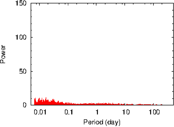
The band differential magnitude () in the sense ‘’ were plotted as a function of Julian date to generate LCs of the target stars and to identify variables. In the first step, we visually checked all the LCs for any variability. Any star which exhibited a systematic visual variation larger than the scatter in comparison star is considered as a variable star. There were some stars which do not show any intra-night variability but exhibit night-night variation. In the second step, we used the Period444http://www.starlink.rl.ac.uk/docs/sun167.htx/sun167.html software based on the Lomb-Scargle (LS) periodogram (Lomb, 1976; Scargle, 1982) to determine the periods of all the stars and phase-folded the LCs to identify the periodic variables visually. The LS method is effective even in the case of unevenly sampled data sets which are common in a majority of the astronomical observations. To check whether the data gaps could produce any false periodicity, we performed LS periodogram analysis on the periodic star after randomizing its amplitude by using linux command-line utility i.e., shuf555http://www.gnu.org/software/coreutils/shuf. None of the power spectra of randomized LC of identified periodic variables show any periodic signature. As an example, power spectra of the periodic variable V56 and its randomized LC are shown in Fig. 4. The maximum power is found at 0.173 day for this periodic variable whereas no signature of periodicity is visible in the randomized LC. We have also verified the periods using the NASA Exoplanet Archive Periodogram service666https://exoplanetarchive.ipac.caltech.edu/cgi-bin/Pgram/nph-pgram and PERIOD04777http://www.univie.ac.at/tops/Period04 (Lenz & Breger, 2005). The periods obtained using these programs generally matched well. Once the periodic variables were identified, the remaining LCs were once more checked visually to identify non-periodic variables.
The RMS dispersion of the magnitudes as a function of mean instrumental magnitude for all the target stars is shown in Fig. 5. As expected the dispersion increases towards the fainter end. Identified variables are shown with filled (periodic) and open (non-periodic) circles. Some of the stars with a very high rms in Fig 5 were not designated as variables due to unusual high photometric errors (possible reason may be bad pixels, bright background of the nearby star, residual from the cosmic corrections, etc) as compared to stars in the same magnitude bin or large deviation in magnitude estimation. These stars were further checked visually to ascertain the variability.

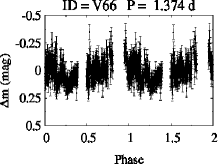
We identified 47 and 24 stars as periodic and non-periodic variables. The identification number, coordinates, period and other parameters of the identified variables are listed in Table LABEL:Variables. The periods and amplitude of the variables range between 4 hrs and 18 days and from 0.1 to 2.0 magnitude, respectively. The optical CMD as discussed in Section 3.3 will further be used to classify the identified variables as PMS members or field stars (cf. next section). Therefore, the LCs of most of the variables (66) will be discussed in ensuing sections except for five having no band detection, i.e., V41, V42, V66, V68 and V71. The LCs of these variables are shown in Appendix A. For the two variables (V26 and V43; cf. Table LABEL:Variables) without band photometry, we transformed their available magnitudes (g, r, i) to and magnitudes using the available transformation equations888https://www.sdss.org/dr12/algorithms/sdssubvritransform/.


3.5 Determination of physical parameters of the variables
3.5.1 Through HR diagram
Fig. 6 shows CMD for 66 variables where open and filled circles denote non-periodic and periodic variables, respectively. The post-MS isochrone (black thick curve) and the PMS isochrones are the same as in Fig. 3. The evolutionary tracks of different masses (black dotted curves) by Siess et al. (2000) are also shown. All the isochrones and evolutionary tracks are corrected for the distance and reddening (cf. Section 3.3). Seventeen of the variables show excess IR emission, whereas fifteen of the variables are cluster members as determined from membership probability. These are shown with red star and blue square symbols, respectively. Most of these variables have ages 2 Myr with an upper age limit of 7 Myr, as discussed in Section 3.3. Therefore, 49 variables (29 periodic) having age Myr are considered to be PMS stars associated with Sh 2-170 (red symbols). Remaining 17 variables (15 periodic) are considered as non-member MS/field stars (black symbols).
The individual age and mass of each PMS variables can be determined from their position in the CMD by using the procedure discussed by Chauhan et al. (2009) and Sharma et al. (2017). The estimated age and mass of the PMS variables and the YSOs are given in Table LABEL:Variables and Table LABEL:YSO, respectively. The age and mass distributions of the PMS variables are shown in Fig. 7. The age distribution shows a peak around 1 Myr and an age spread of up to 7 Myr. Average age and mass of the 49 PMS variables associated with Sh 2-170 are found to be 2.40.6 Myr and 1.30.1 M⊙, respectively.


3.5.2 Through spectral energy distribution
We constructed SEDs of the PMS variables using the grid models and fitting tools of Whitney et al. (2003b, a, 2004) and Robitaille et al. (2006, 2007) to characterise and understand their nature. This method has been extensively used in our previous studies (see. e.g., Jose et al., 2016; Sharma et al., 2017, and references therein). We were able to construct SEDs for the 43 PMS variables using the available optical, NIR (2MASS) and MIR (WISE, ) data, with a condition that each star should have photometric data at least in five bands. The SED fitting tool fits each of the models to the data allowing the distance and extinction as free parameters. The distance for the region is taken as kpc (cf. Section 3.3) and we varied in a range 2.2 to 30 mag (Bhatt et al., 2012). We further set photometric uncertainties of 10% for the optical and 20% for both the NIR and MIR data. These values are adopted instead of the formal errors in the catalog in order to fit without any possible biases caused by underestimating the flux uncertainties. We obtained the physical parameters of the PMS variables using the relative probability distribution for the stages of all the ‘well-fit’ models. The well-fit models for each source are defined by 2, where is the goodness-of-fit parameter for the best-fit model and is the number of input data points. In Fig. 8, we show example SEDs for the two PMS variables, where the solid black curves represent the best-fit and the grey curves are the subsequent well-fits. Table LABEL:Variables and Table LABEL:YSO list the age, mass and other relevant parameters of the PMS variables and YSOs estimated from the SED analysis. The average age and mass of the 43 PMS variables are found to be Myr and M⊙, respectively. These values are comparable within errors to those derived from the CMD (age=2.40.6 Myr, mass=1.30.1 M⊙).


3.6 Classification of the identified variable stars
The association of the 71 identified variables with Sh 2-170 has been checked on the basis of their membership probability (cf. Section 3.2), the position in the CMD (cf. Section 3.5.1), and the presence or absence of excess IR emission (cf. Section 3.3), and the details about their classification and nature of variability are given in Table LABEL:variability_nature. Periodic/non-periodic nature of the variables are also mentioned in the table. Five of the identified variables could not be classified due to non-availability of their band data. Out of the remaining 66 variables, 44 (66%) exhibit periodicity. Forty nine variables are found to be PMS sources, of which 29 (59%) variables are periodic. Most of the PMS variables have age and mass in the range of 0.1 - 2 Myr and 0.2 - 3 M⊙, indicating that they are most probably T-Tauri stars. Seventeen of them exhibit excess IR emission and are classified as Class ii sources (cf. Section 3.3). The remaining 32 PMS variable stars having either insignificant or no IR-excess, may belong to the Class iii category. Seventeen stars are found to be MS/field stars and 15 (88%) of them have periodic LCs.
3.6.1 MS/field variables
The variability in MS population is mainly caused by pulsation. The MS variability of various kind of pulsators like Cep, Scuti, SPB, Doradus etc. has been extensively studied (e.g., Balona et al., 1997; Balona & Dziembowski, 2011; Handler & Meingast, 2011; Mowlavi et al., 2013). A new class of variable stars situated in the HR diagram between the red end of SPB and the blue end of Scuti, where stars are not expected to occur according to the classical stellar models, are also reported (see e.g., Mowlavi et al., 2013; Lata et al., 2014).
We have identified 17 MS/field variables and 15 of them are periodic having periods in the range 4 hrs - 6 days and band amplitudes of 0.35 - 1.58 mag. Their respective phase-folded LCs are shown in Fig. 9. A higher percentage of periodic variables in the MS/field stars is natural as their variability is dominated by their pulsating behaviour (Balona et al., 1997; Balona & Dziembowski, 2011). The LCs of V48, V61 and V64 clearly show two dips which resemble to those of Lyrae type binary stars. The Lyrae type systems are composed of two stars typically with different evolutionary states. The binaries are in a tight orbit and mass transfer can take place in semi-detached systems (Hoffman et al., 2008). V48 and V61 show similar periods of about 15 hrs with amplitudes of 0.87 and 0.7 mag, respectively. V64 shows a little longer period of about 1 day with an amplitude of 0.85 mag. The Lyrae type variables generally have periods longer than 1 day (Hoffman et al., 2008) with few exceptions (e.g., 0.29 days for HD 105575 and 198.5 days for HD 105998999http://www.sai.msu.su/gcvs/cgi-bin/search.cgi?search=W+Cru). The secondary dip (0.39 mag) in V48 is less than half of the primary dip (0.87 mag). A small ‘bump’ could also be seen around the secondary dip. In Fig. 10. We also show the remaining LCs of 2 non-periodic MS/field stars showing variations in the range 1.1 - 1.4 mag.
To further characterise these MS/field variables, we plot in
Fig. 11 their effective
temperature () versus bolometric luminosity (L/L⊙)
HR diagram. The absolute magnitudes were estimated by using the distance given by Bailer-Jones et al. (2018) and
Gaia
Collaboration et al. (2018, 2016) and assuming the normal extinction law
(Milne &
Aller, 1980; Gottlieb &
Upson, 1969).
The absolute magnitudes of these stars are then matched with those given in the theoretical MS by
Pecaut &
Mamajek (2013)101010http://www.pas.rochester.edu/
emamajek/EEM_dwarf_UBVIJHK_colors_Teff.txt and
the corresponding values of and L/L⊙ are taken.
The associated errors could be due to uncertainty in theoretical models, parallax values and/or in the extinction values.
Fig. 11 indicates that V29 is a Scuti star (blue dotted region).
The amplitude and period of this star are 0.43 mag and 20 hrs, respectively.
V8 lies in between the SPB and Scuti regions. This one could be a variable of a new class.
Its amplitude in band and period are 0.35 mag and 6.3 days, respectively.
The remaining stars are of lower surface temperature/mass (9000K/2M⊙ - 4000K/0.6M⊙).
Detailed analysis of these MS/field variables are beyond the scope of this study in which we try to concentrate mainly on
variability of PMS stars, as discussed in detail in the next section.


4 DISCUSSION: PRE-main-sequence VARIABLES
The circumstellar disc plays a significant role in the photometric variation of both periodic and non-periodic PMS stars. Accretion and dust obscuration are responsible for most of the irregular variations in young stars (Herbst et al., 1994). Spot (both hot and cool) modulation is the most common cause of periodic variation. CTTSs have a thick disc, from which magnetically guided accretion give rise to strong emission. Erratic enhanced accretion causes hot spots on the stellar surface, which can lead to large amplitude variations. In WTTS the disc is more or less depleted and the accretion is inactive. Instead developed cool spots on the stellar surface emerges as the major modulator of variability.
PMS stars with different masses have different amount of circumstellar disk material around them. Also they undergo mass-dependent evolution of the internal structure, which determines the dynamo process inducing stellar magnetic activities (Donati & Landstreet, 2009). This not only influences the accretion but also controls the stellar rotation through disc-locking. In the disc-locking scenario (Koenigl, 1991) the disc-star interaction results in the transfer of angular momentum from the star to the circumstellar disc and consequently the star maintains almost a constant rotation rate until the coupling breaks due to the significant dissipation of the disc. The angular momentum could also be released through an enhanced stellar wind powered by the accretion of material from the disc (Matt & Pudritz, 2005b). In both the cases a correlation between rotation speed and presence of disc is expected in the sense that slow rotators must be surrounded by substantial circumstellar disc, whereas fast rotators should be in a process of disc dispersal. We discuss variability characteristics of the PMS stars in our sample in the subsequent subsections.


4.1 Periodic PMS variables: An insight into disc-locking
PMS stars are supposed to release their angular momentum through different mechanisms as they make the transition from the protostellar state down to MS. Disc-locking is the most commonly invoked mechanism to regulate the angular momentum (see e.g., Herbst et al., 2000). Herbst et al. (2000); Herbst et al. (2002) have found a bimodal period distribution around 1 and 8 days for PMS variables with M > 0.25 M⊙ in Orion Nebula Cluster (ONC). Several studies (e.g., Herbst et al., 2000) explained this bimodal distribution through disc-locking mechanism. If a star is disc-locked further increase in its rotation speed due to contraction would be slowed down and a significant number of star will end up having similar rotation periods. After released from disc-locking, the stars will again increase their rotation speed.
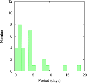
Twenty nine of our PMS variable stars show periodicity in their LCs. In Fig. 12 and Fig. 13, we have plotted the phase folded LC of Class ii (10) and Class iii (19) periodic variables, respectively. In general the periods and amplitudes of Class ii variables are larger than Class iii variables. All the Class iii variables have period 6 days. As the variability signatures in WTTSs are dominated by the asymmetric distribution of cool spots on the stellar surface, 19 Class iii sources showing periodicity in the range of 4 hrs to 6 days with amplitudes of 0.15-0.68 mag (with an exception of V32 having an amplitude of 1.38 mag) are classified as WTTSs (see also, Bhardwaj et al., 2019). We show the period distribution for all 29 periodic PMS stars in the upper panel of Fig. 14. The distribution is bimodal with peaks near 1.5 and 4.5 days. We further subdivided this sample into Class ii and Class iii sources and their period distributions are also shown in the lower panel of Fig. 14. The bimodality is more clearly visible for Class iii sources, whereas the period distribution for the Class ii sources is more or less flat. Here we would like to mention that uneven sampling and lack of observations for longer periods may be the reason for the small number of relatively slow rotators. Lamm et al. (2005) have also found a similar bimodal period distribution for variables having 1.3 (mass 0.25 M⊙) with peaks at 1 and 4 days in NGC 2264. In the case of IC 348, Littlefair et al. (2005) have found a bimodal period distribution around 3 and 8 days similar to that seen in ONC for the stars having masses 0.25 M⊙, but have reported a statistically significant lack of rapidly rotating stars with respect to the ONC. They also concluded that in spite of the similarity in the ages and disc fractions between NGC 2264 and IC 348, the marked difference in the period distributions between the two clusters presents a serious challenge to the disc-locking paradigm, as it provides no explanation for the difference. However, differences in the cluster environments and the physical conditions leading to the star formation can lead to these observed differences in the period distribution (see also, Littlefair et al., 2005).
Here, we would also like to mention the peculiar LC of V34 as shown in Fig. 15. In addition to the inter-night variability it also shows small intra-night variability. In the same night (within few hours) we see a small change in brightness in a periodic fashion. Multiple physical phenomena such as spot modulation, inner disc co-rotation and extinction events could be responsible for this.

4.2 Non-periodic PMS variables: Bursters and faders
An increase in accretion rate from the circumstellar disc onto the star can give rise to a significant burst in magnitude (few mags) that lasts over hours to days (Cody & Hillenbrand, 2018). Similarly, variable circumstellar extinction can cause brightening/fading events of a few tenths of magnitude. They are of short phenomena of up to a few hours typically (for e.g., AA Tau, Guo et al., 2018).
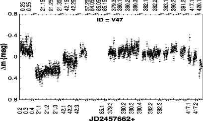
Twenty of our PMS variable stars do not show periodicity in their LCs. In Fig. 16 and Fig. 17, we have plotted the LCs of Class ii (7) and Class iii (13) non-periodic variables, respectively. Their amplitudes vary between 0.1 - 2 mag. The Class ii variables show significantly large magnitude variations as compared to the Class iii variables. Also, their variability features include either single or multiple fading/brightening events that last for different time-spans.These seven Class ii variables are therefore classified as CTTSs (see also, Bhardwaj et al., 2019). The photometric variations of these sources are found to be in between 0.5 mag to 2.0 mag. The source V35 shows a huge variation of 2 mag . On Nov 2016 it showed a decrease in magnitude from its semi-stable maximum. Again on Oct 2017 it showed a larger decrease, and with a few fluctuations reached to its stable maximum brightness around Nov 2017. The source V27 is almost stable in most part of its LC with little fluctuation. After Oct 2017 it started fluctuating with a maximum magnitude decrease of around 1 mag on Nov 2017. In the case of V14 and V36 we see significant intra-night fading and brightening events in few nights. We don’t see any intra-night variation in V19, but inter-night variations are present in night to night with a maximum variation of 0.87 mag. The characteristics of variability found in these sources are typical of CTTSs.


4.3 Correlation of periods/amplitudes of variables with their stellar parameters
To check the dependence of the variation of the PMS variables on their evolutionary status, in Fig. 18 we plot the normalized cumulative amplitude distribution of Class ii and Class iii sources. This distribution clearly indicates that Class ii sources exhibit larger amplitude variations as compared to Class iii sources with a 96% confidence level as calculated by the Kolmogorov–Smirnov test. Similar results have been reported by Lata et al. (2011, 2012) and Bhardwaj et al. (2019). To further investigate how the period of variability evolves with the age and how the mass of PMS stars influence their periods, we plot the period of the PMS variables as a function of age and mass in the left and right panels of Fig. 19, respectively. The left panel of Fig. 19 indicates that stars with periods up to 6 days are uniformly distributed for the entire range of ages of the PMS sources, whereas all the PMS variables having periods 6 days are younger than 2 Myr. Lata et al. (2014); Lata et al. (2016) have also found a similar result that PMS stars with age 3 Myr seem to be relatively fast rotators. The right panel of Fig. 19 displays the dependence of period on the stellar mass. Although the sample is small, but we can see a trend in the distribution: out of 5 slow rotators (period 6 days), 4 have masses less than 1 M⊙. and variables with periods 6 days have masses 2 M⊙, whereas out of 3 high mass variables (M 3 M⊙), 2 have periods 1 days. A similar trend has been reported by Lata et al. (2014); Lata et al. (2016). Littlefair et al. (2005) have also found a strong correlation between stellar mass and rotation rate in the case of IC 348. They concluded that the strong mass dependence of rotation rate seen in ONC (Herbst et al., 2000) may well be a common feature of young stellar populations.
Fig. 20 plots amplitude of variability as a function of age and mass of the PMS variables, which roughly indicates that their amplitudes decrease with the increase in mass and age. This is similar to the previous findings (Herbst et al., 2000; Herbst et al., 2002; Littlefair et al., 2005; Lata et al., 2014; Lata et al., 2016). The amplitude decrease with age could be due to the dispersal of the disc. The present result further supports that of our previous studies (Lata et al., 2011, 2012, 2016) that the disc dispersal mechanism is less efficient for relatively low mass stars and that a significant amount of discs is dispersed by 5 Myr. This is also in accordance with the result obtained by Haisch et al. (2001).


4.4 Correlation of periods/amplitudes of PMS variables with disc evolution
To understand the influence of circumstellar discs on the period and amplitude of young stars, we have to first identify a suitable disc indicator. Various disc indicators, such as equivalent widths of emission line and Ca II triplet lines, and indices, disc fraction, etc., have been used in the previous studies (e.g., Herbst et al., 2000; Littlefair et al., 2005; Cieza & Baliber, 2007). Since band fluxes originate solely from the photosphere unlike band flux which originates in circumstellar disc emission as well as photospheric emission, this provides index with a longer wavelength base compared to other NIR indices (e.g. or ). This index is expressed as (cf. Hillenbrand et al., 1998):
| (4) |
where is the observed colour of the star, is the intrinsic colour and and are the interstellar extinction in the and bands, respectively. We have used the value ( mag) as determined by using parameter (Johnson & Morgan, 1953) to correct the stars for their extinction. Intrinsic colour of the variables were taken from the PMS isochrones of Siess et al. (2000) according to the age and mass as derived by their CMD and then corrected for the distance and extinction.
Since is sensitive to the inner part of the disc, we also used the available MIR data of these variables to compute an MIR index , which is a better indicator of the presence of disc and its evolution (Lada et al. 2000; Rodríguez-Ledesma et al. 2010). Since the presence of disc also induces the accretion activity, we have also used the information such as the disc accretion rate and the disc mass obtained from the SED fitting tool (cf. Sec 3.5.2). The upper panels of Fig. 21 show the variation of amplitude as a function of and . A trend can be clearly seen in the sense that the larger values of the disc indicators, i.e., or correspond to relatively larger amplitude variations. The versus amplitude diagram manifests that Class ii sources have active circumstellar discs as compared to Class iii sources, hence these sources display more active and dynamic variability due to the accretion activities. In the case of NGC 2282, Dutta et al. (2018) have also reported a positive correlation between RMS amplitudes and / disc indicators. The lower panels of Fig. 21 show amplitudes as a function of the disc accretion rate and disc mass, which indicates that higher disc accretion activity ( M) induces higher amplitude variation. The amplitude variation also depends on the mass of the stellar disc in the sense that discs with mass M⊙ show relatively larger amplitude variation.

The extensive study of rotation rates in ONC carried out by Herbst et al. (2000); Herbst et al. (2002) reveals a strong correlation between rotation period and infrared excess, suggesting that the observed rotation period distribution could be due to the disc-locking mechanism. In Fig. 22 (upper panels) we plot rotation period as a function of the and disc indicators. The MIR disc indicator clearly suggests that all the five slow rotators (having periods 6 days) are Class ii sources having higher value of index (0.4 mag), whereas Class iii sources with 0.0 mag have periods 6 days. This result indicates a reasonable likelihood that the presence of disc affects the rotation of the star. Similar results were reported by Edwards et al. (1993) and the physical interpretation proposed by the authors was that the discs slows the rotation of stars through magnetic interaction (Koenigl, 1991; Ostriker & Shu, 1995). Hence, stars having discs either locked or recently released tends to be slower rotators than stars which already dispersed their disc. However, Littlefair et al. (2005) did not find any correlation between the equivalent width or excess and the rotation period of the stars. They cautioned that the correlation between rotation period and infrared excess expressed by index can also arise due to the strong dependence of on stellar mass in the sense that high-mass stars have larger values as compared to low-mass stars (Hillenbrand et al., 1998). To check the dependence of and NIR/ MIR excess on stellar mass, we plot these parameters in the bottom panels of Fig. 22. The plots indicate a weak correlation between NIR/ MIR excess with stellar mass in the sense that higher values of NIR/MIR excess are associated with relatively low mass stars. Hence relatively low mass stars are preferably slow rotators.
Cieza & Baliber (2007) reported a clear increase of the disc fraction with period of stars in ONC and NGC 2264. They showed that the long-period peak (P 8 days) of the bimodal distribution observed in ONC is dominated by the population of stars possessing a disc, while the short-period peak (P 2 days) is dominated by the discless population and concluded that this is a strong evidence that the star-disc interaction regulates the angular momentum of young stars.
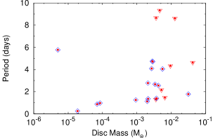
Fig. 23 shows the effect of disc accretion rate and stellar disc mass on the period. It is evident from this figure that both the disc accretion rate and stellar disc mass affects the stellar rotation in the sense that slow rotators are highly accreting stars (disc accretion rate 5 M ) and have higher stellar disc mass ( 3 M⊙ ).
5 Summary and conclusion
In this paper we have presented the multi-epoch deep band (20 mag) photometric monitoring of the Sh 2-170 region to understand the characteristics of variables in the region. Following are the main results.
-
•
We have identified 71 variables in the region. The probable members associated with Sh 2-170 are identified on the basis of their PM, location in the optical CMD and presence or absence of excess IR emission. Forty nine variables are found to be probable PMS stars, whereas remaining 17 stars are found to be MS/field population. Of 49 PMS variables, 17 and 32 are classified as Class ii and Class iii sources, respectively. Ten and nineteen of Class ii and Class iii variables are found to be periodic; 15 MS variables are found to be periodic.
-
•
The majority of the PMS variables have mass and age in the range of 0.2 M/M⊙ 3.0 and 0.1 - 2.0 Myrs, respectively, and hence should be TTSs. The rotation period of the PMS variables ranges from 4 hrs to 18 days whereas the amplitude varies from 0.1 mag to 2.0 mag. The amplitude is larger in Class ii sources (up to 2.0 mag) as compared to those in Class iii sources (0.7 mag).
-
•
The period distribution of the PMS stars reveals a bimodal nature with peaks at 1.5 days and 4.5 days. The period for Class ii sources ranges from 1 to 18 days, whereas Class iii sources have periods in the range 4 hrs - 6 days. The correlation between stellar rotation period and NIR/MIR excess is apparent in the sense that slow rotators have larger NIR/MIR excesses as compared to fast rotators. It is also found that the disc accretion rate and stellar disc mass are correlated to the stellar rotation in the sense that highly accreting stars (disc accretion rate 5 M) as well as stars of higher disc mass ( 3 M⊙) are preferably slow rotators.
-
•
The bimodal period distribution and dependence of rotation period on IR excess/accretion rate/disc mass are compatible with the disc-locking model. This model suggests that when a star is disc-locked, its rotation speed doesn’t change and when the star is released from the locked-up disc, it can spin up with its contraction.
-
•
Both the period and amplitude of PMS variables decrease with increasing stellar mass. This is in accordance with our earlier proposition that the decrease in variability amplitude in relatively massive stars could be due to the dispersal of circumstellar disc and that the mechanism of this disc dispersal operates less efficiently in relatively low mass stars (Lata et al., 2011; Lata et al., 2014; Lata et al., 2016).
-
•
The amplitude of variables is correlated with the NIR and MIR disc indicators in the sense that the larger value of disc indicators, i.e., or , corresponds to relatively larger amplitude variation. The disc indicator manifests that Class ii sources have active circumstellar disc around them as compared to Class iii sources, hence these sources are more active and dynamic and display larger variability due to the accretion activities. The amplitude of variability also depends on the disc accretion rate and disc mass in the sense that higher disc accretion activity ( M) and massive discs of M⊙ induce higher amplitude variation.
-
•
These results are also in agreement with the notion that cool spots on WTTSs are responsible for most or all of their variations, while hot spots on CTTSs resulting from variable mass accretion from the inner disc contribute to their larger amplitudes and more irregular behaviours.
Here, we would like to emphasize that cool spots on the surface of a WTTS can change their shapes and distribution on a timescale of months, which makes it impossible to maintain the integrity of phase over different observing seasons (Herbst et al., 2000). In future studies, observations in a larger number of nights preferably within an observing season will be useful to determine the periods of PMS stars more accurately and to obtain statistically more significant samples of PMS variables. Also desirable are the observing in different cluster environment.
Acknowledgment
We are very thankful to the referee Prof. William Herbst for the critical review of the manuscript and useful comments. The observations reported in this paper were obtained by using the 1.3m Devasthal Fast Optical Telescope (DFOT, India), 0.7m TRT-GAO (Thai Robotic Telescope at Gao Mei Gu Observatory, China) and 0.5m telescope of Thai National Observatory (TNO, Thailand). This work made use of data from the Two Micron All Sky Survey (a joint project of the University of Massachusetts and the Infrared Processing and Analysis Center/California Institute of Technology, funded by the National Aeronautics and Space Administration and the National Science Foundation), and archival data obtained with the Space Telescope and Wide Infrared Survey Explorer (operated by the Jet Propulsion Laboratory, California Institute of Technology, under contract with the NASA. This publication also made use of data from the European Space Agency (ESA) mission (https://www.cosmos.esa.int/gaia), processed by the Data Processing and Analysis Consortium (DPAC, https://www.cosmos.esa.int/web/gaia/dpac/consortium). Funding for the DPAC has been provided by national institutions, in particular the institutions participating in the multilateral agreement. AKP is thankful to NARIT, Thailand for the support during the stay at NARIT.
References
- Aarnio et al. (2009) Aarnio A. N., Stassun K. G., Matt S. P., 2009, in Stempels E., ed., American Institute of Physics Conference Series Vol. 1094, 15th Cambridge Workshop on Cool Stars, Stellar Systems, and the Sun. pp 337–340, doi:10.1063/1.3099114
- Aarnio et al. (2010) Aarnio A. N., Stassun K. G., Matt S. P., 2010, ApJ, 717, 93
- Aarnio et al. (2011) Aarnio A. N., Stassun K. G., Hughes W. J., McGregor S. L., 2011, Sol. Phys., 268, 195
- Appenzeller & Mundt (1989) Appenzeller I., Mundt R., 1989, A&ARv, 1, 291
- Bailer-Jones et al. (2018) Bailer-Jones C. A. L., Rybizki J., Fouesneau M., Mantelet G., Andrae R., 2018, AJ, 156, 58
- Balona & Dziembowski (2011) Balona L. A., Dziembowski W. A., 2011, MNRAS, 417, 591
- Balona et al. (1997) Balona L. A., Dziembowski W. A., Pamyatnykh A., 1997, MNRAS, 289, 25
- Bhardwaj et al. (2019) Bhardwaj A., Panwar N., Herczeg G. J., Chen W. P., Singh H. P., 2019, arXiv e-prints, p. arXiv:1906.00256
- Bhatt et al. (2012) Bhatt H., Sagar R., Pandey J. C., 2012, New Astron., 17, 160
- Chauhan et al. (2009) Chauhan N., Pandey A. K., Ogura K., Ojha D. K., Bhatt B. C., Ghosh S. K., Rawat P. S., 2009, MNRAS, 396, 964
- Cieza & Baliber (2007) Cieza L., Baliber N., 2007, ApJ, 671, 605
- Cody & Hillenbrand (2018) Cody A. M., Hillenbrand L. A., 2018, AJ, 156, 71
- Cutri et al. (2003) Cutri R. M., et al., 2003, VizieR Online Data Catalog, 2246
- Donati & Landstreet (2009) Donati J. F., Landstreet J. D., 2009, ARA&A, 47, 333
- Dutta et al. (2018) Dutta S., Mondal S., Joshi S., Jose J., Das R., Ghosh S., 2018, MNRAS, 476, 2813
- Edwards et al. (1993) Edwards S., et al., 1993, AJ, 106, 372
- Gaia Collaboration et al. (2016) Gaia Collaboration et al., 2016, A&A, 595, A1
- Gaia Collaboration et al. (2018) Gaia Collaboration et al., 2018, A&A, 616, A1
- Girard et al. (1989) Girard T. M., Grundy W. M., Lopez C. E., van Altena W. F., 1989, AJ, 98, 227
- Gottlieb & Upson (1969) Gottlieb D. M., Upson II W. L., 1969, ApJ, 157, 611
- Guo et al. (2018) Guo Z., et al., 2018, ApJ, 852, 56
- Gutermuth et al. (2005) Gutermuth R. A., Megeath S. T., Pipher J. L., Williams J. P., Allen L. E., Myers P. C., Raines S. N., 2005, ApJ, 632, 397
- Gutermuth et al. (2009) Gutermuth R. A., Megeath S. T., Myers P. C., Allen L. E., Pipher J. L., Fazio G. G., 2009, ApJS, 184, 18
- Haisch et al. (2001) Haisch Karl E. J., Lada E. A., Lada C. J., 2001, ApJ, 553, L153
- Handler & Meingast (2011) Handler G., Meingast S., 2011, A&A, 533, A70
- Herbst et al. (1994) Herbst W., Herbst D. K., Grossman E. J., Weinstein D., 1994, AJ, 108, 1906
- Herbst et al. (2000) Herbst W., Maley J. A., Williams E. C., 2000, AJ, 120, 349
- Herbst et al. (2002) Herbst W., Bailer-Jones C. A. L., Mundt R., Meisenheimer K., Wackermann R., 2002, A&A, 396, 513
- Herbst et al. (2007) Herbst W., Eislöffel J., Mundt R., Scholz A., 2007, Protostars and Planets V, pp 297–311
- Hillenbrand (2002) Hillenbrand L. A., 2002, arXiv Astrophysics e-prints,
- Hillenbrand et al. (1998) Hillenbrand L. A., Strom S. E., Calvet N., Merrill K. M., Gatley I., Makidon R. B., Meyer M. R., Skrutskie M. F., 1998, AJ, 116, 1816
- Hoffman et al. (2008) Hoffman D. I., Harrison T. E., Coughlin J. L., McNamara B. J., Holtzman J. A., Taylor G. E., Vestrand W. T., 2008, AJ, 136, 1067
- Johnson & Morgan (1953) Johnson H. L., Morgan W. W., 1953, ApJ, 117, 313
- Jose et al. (2016) Jose J., Kim J. S., Herczeg G. J., Samal M. R., Bieging J. H., Meyer M. R., Sherry W. H., 2016, ApJ, 822, 49
- Koenig & Leisawitz (2014) Koenig X. P., Leisawitz D. T., 2014, ApJ, 791, 131
- Koenigl (1991) Koenigl A., 1991, ApJ, 370, L39
- Lada et al. (2000) Lada C. J., Muench A. A., Haisch Jr. K. E., Lada E. A., Alves J. F., Tollestrup E. V., Willner S. P., 2000, AJ, 120, 3162
- Lamm et al. (2005) Lamm M. H., Mundt R., Bailer-Jones C. A. L., Herbst W., 2005, A&A, 430, 1005
- Lata et al. (2011) Lata S., Pandey A. K., Maheswar G., Mondal S., Kumar B., 2011, MNRAS, 418, 1346
- Lata et al. (2012) Lata S., Pandey A. K., Chen W. P., Maheswar G., Chauhan N., 2012, MNRAS, 427, 1449
- Lata et al. (2014) Lata S., Yadav R. K., Pandey A. K., Richichi A., Eswaraiah C., Kumar B., Kappelmann N., Sharma S., 2014, MNRAS, 442, 273
- Lata et al. (2016) Lata S., Pandey A. K., Panwar N., Chen W. P., Samal M. R., Pandey J. C., 2016, MNRAS, 456, 2505
- Lenz & Breger (2005) Lenz P., Breger M., 2005, Communications in Asteroseismology, 146, 53
- Littlefair et al. (2005) Littlefair S. P., Dhillon V. S., Martín E. L., 2005, A&A, 437, 637
- Lomb (1976) Lomb N. R., 1976, Ap&SS, 39, 447
- Makidon et al. (2004) Makidon R. B., Rebull L. M., Strom S. E., Adams M. T., Patten B. M., 2004, AJ, 127, 2228
- Marigo et al. (2008) Marigo P., Girardi L., Bressan A., Groenewegen M. A. T., Silva L., Granato G. L., 2008, A&A, 482, 883
- Matt & Pudritz (2004) Matt S., Pudritz R. E., 2004, ApJ, 607, L43
- Matt & Pudritz (2005a) Matt S., Pudritz R. E., 2005a, MNRAS, 356, 167
- Matt & Pudritz (2005b) Matt S., Pudritz R. E., 2005b, ApJ, 632, L135
- Matt & Pudritz (2008a) Matt S., Pudritz R. E., 2008a, ApJ, 678, 1109
- Matt & Pudritz (2008b) Matt S., Pudritz R. E., 2008b, ApJ, 681, 391
- Milne & Aller (1980) Milne D. K., Aller L. H., 1980, AJ, 85, 17
- Mowlavi et al. (2013) Mowlavi N., Barblan F., Saesen S., Eyer L., 2013, A&A, 554, A108
- Najita (1995) Najita J., 1995, in Lizano S., Torrelles J. M., eds, Revista Mexicana de Astronomia y Astrofisica Conference Series Vol. 1, Revista Mexicana de Astronomia y Astrofisica Conference Series. p. 293
- Ostriker & Shu (1995) Ostriker E. C., Shu F. H., 1995, ApJ, 447, 813
- Pecaut & Mamajek (2013) Pecaut M. J., Mamajek E. E., 2013, ApJS, 208, 9
- Percy et al. (2006) Percy J. R., Gryc W. K., Wong J. C.-Y., Herbst W., 2006, PASP, 118, 1390
- Percy et al. (2010) Percy J. R., Grynko S., Seneviratne R., Herbst W., 2010, PASP, 122, 753
- Robitaille et al. (2006) Robitaille T. P., Whitney B. A., Indebetouw R., Wood K., Denzmore P., 2006, ApJS, 167, 256
- Robitaille et al. (2007) Robitaille T. P., Whitney B. A., Indebetouw R., Wood K., 2007, ApJS, 169, 328
- Rodríguez-Ledesma et al. (2010) Rodríguez-Ledesma M. V., Mundt R., Eislöffel J., 2010, A&A, 515, A13
- Roger et al. (2004) Roger R. S., McCutcheon W. H., Purton C. R., Dewdney P. E., 2004, A&A, 425, 553
- Russeil et al. (2007) Russeil D., Adami C., Georgelin Y. M., 2007, A&A, 470, 161
- Scargle (1982) Scargle J. D., 1982, ApJ, 263, 835
- Sharma et al. (2016) Sharma S., et al., 2016, AJ, 151, 126
- Sharma et al. (2017) Sharma S., Pandey A. K., Ojha D. K., Bhatt H., Ogura K., Kobayashi N., Yadav R., Pandey J. C., 2017, MNRAS, 467, 2943
- Shu et al. (1994) Shu F. H., Najita J., Ruden S. P., Lizano S., 1994, ApJ, 429, 797
- Siess et al. (2000) Siess L., Dufour E., Forestini M., 2000, A&A, 358, 593
- Skrutskie et al. (2006) Skrutskie M. F., et al., 2006, AJ, 131, 1163
- Stetson (1987) Stetson P. B., 1987, PASP, 99, 191
- Stetson (1992) Stetson P. B., 1992, in Worrall D. M., Biemesderfer C., Barnes J., eds, Astronomical Society of the Pacific Conference Series Vol. 25, Astronomical Data Analysis Software and Systems I. p. 297
- Werner et al. (2004) Werner M. W., et al., 2004, ApJS, 154, 1
- Whitney et al. (2003a) Whitney B. A., Wood K., Bjorkman J. E., Wolff M. J., 2003a, ApJ, 591, 1049
- Whitney et al. (2003b) Whitney B. A., Wood K., Bjorkman J. E., Cohen M., 2003b, ApJ, 598, 1079
- Whitney et al. (2004) Whitney B. A., Indebetouw R., Bjorkman J. E., Wood K., 2004, ApJ, 617, 1177
- Wright et al. (2010) Wright E. L., et al., 2010, AJ, 140, 1868
- Yadav et al. (2013) Yadav R. K. S., Sariya D. P., Sagar R., 2013, MNRAS, 430, 3350
- van den Ancker et al. (1998) van den Ancker M. E., de Winter D., Tjin A Djie H. R. E., 1998, A&A, 330, 145
| ID | Flag | Parallax | Probability | ||||||||
|---|---|---|---|---|---|---|---|---|---|---|---|
| (mag) | (mag) | (mas/yr) | (mas/yr) | (mas) | (%) | (mag) | (mag) | ||||
| M1 | 0.394085 | 64.623123 | — — | — — | — | -2.6403 0.0538 | -0.5290 0.1046 | 0.2530 0.0400 | 100 | 12.525 | — |
| M2 | 0.407023 | 64.626556 | 18.430 0.071 | 16.258 0.043 | a | -2.6724 0.1730 | -0.4744 0.1477 | 0.3230 0.1050 | 99 | 17.800 | 1.921 |
| M3 | 0.446222 | 64.629654 | — — | — — | — | -3.1729 0.9959 | -0.4800 0.6734 | -0.0480 0.4665 | 85 | 20.017 | 2.091 |
| M4 | 0.441568 | 64.624008 | 19.676 0.054 | 17.184 0.034 | a | -3.0820 0.4108 | -0.5451 0.2632 | 0.1190 0.1898 | 95 | 18.693 | 2.219 |
a : and data taken from Bhatt
et al. (2012). ;
b : and data taken from the present observations.
| Table | ||||||||||||||||||
|---|---|---|---|---|---|---|---|---|---|---|---|---|---|---|---|---|---|---|
| ID | Flag | Period | Amplitude | RMS | Age | Mass | Data points* | Age* | Mass* | Disc mass* | Disc accretion rate* | |||||||
| (degrees) | (degrees) | (mag) | (mag) | (days) | (mag) | (mag) | (mag) | (mag) | (Myr) | (M⊙) | (Myr) | (M⊙) | (M⊙) | (M⊙ ) | ||||
| V1 | 0.343856 | 64.637985 | 13.9170.027 | 12.2540.013 | a | 0.8660.001 | 0.190.02 | 0.056 | -0.3620.023 | 0.0220.078 | 0.30.1 | 5.40.2 | 14 | 637.1 | 1.40.3 | 3.70.3 | 6.96E-051.31E-04 | 7.06E-111.52E-10 |
| V2 | 0.321549 | 64.498772 | 17.9340.008 | 12.8130.005 | b | — — | 0.370.01 | 0.091 | 2.4370.014 | -0.1800.038 | 0.10.1 | 0.70.1 | 11 | 596.5 | 3.00.1 | 9.60.1 | 9.23E-081.77E-02 | 2.24E-122.17E-19 |
| V3 | 0.241819 | 64.734032 | 13.2300.009 | 12.4500.073 | a | — — | 0.250.10 | 0.078 | 0.1530.089 | — — | 0.60.1 | 5.60.3 | 11 | 102.9 | 1.10.1 | 4.20.1 | 1.39E-071.77E-02 | 1.21E-121.03E-03 |
| V4 | 0.426350 | 64.606903 | 15.2620.014 | 14.4950.043 | a | 0.9710.001 | 0.500.06 | 0.131 | 0.2410.062 | 0.0360.053 | 6.42.2 | 3.10.2 | 10 | 0.4 | 4.82.3 | 3.40.3 | 8.53E-056.56E-04 | 1.84E-101.30E-09 |
a, b : Same as Table 2 ;
c : Converted to and from SDSS data ;
: Parameters derived from CMD ;
* Parameters derived from SED
| Table | |||||||||||||
|---|---|---|---|---|---|---|---|---|---|---|---|---|---|
| ID | Age | Mass | Flag | Data points* | * | Age* | Mass* | Disc mass* | Disc accretion rate* | ||||
| (degrees) | (degrees) | (mag) | (mag) | (Myr) | (M⊙) | (Myr) | (M⊙) | (M⊙) | (M⊙ ) | ||||
| Y1 | 0.386569 | 64.641273 | 16.8400.020 | 14.2820.014 | 0.10.1 | 1.30.1 | a | 13 | 8.9 | 0.30.2 | 4.50.8 | 4.23E-026.37E-02 | 4.57E-078.83E-07 |
| Y2 | 0.399863 | 64.643867 | 19.3240.064 | 17.1130.022 | 1.40.3 | 1.00.1 | a | 13 | 34.5 | 0.10.1 | 4.01.3 | 4.56E-024.75E-02 | 5.57E-077.01E-07 |
| Y3 | 0.405294 | 64.651543 | 18.7950.013 | 16.6740.008 | 1.10.2 | 1.20.1 | a | 13 | 20.0 | 3.82.4 | 3.51.2 | 5.63E-031.98E-02 | 7.84E-084.11E-07 |
| Y4 | 0.676066 | 64.568512 | — — | — — | — — | — — | — | 5 | 0.1 | 1.42.0 | 2.01.3 | 7.92E-032.32E-02 | 8.25E-089.50E-07 |
All the symbols are the same as in Table LABEL:Variables
| Table | |||
|---|---|---|---|
| ID | Type | Comment on Classification | Comment on Variability |
| V1 | PMS/Class iii/WTT | CMD | Periodic |
| V2 | PMS/Class iii | CMD | Non-periodic |
| V3 | PMS/Class iii | CMD | Non-periodic |
| V4 | PMS/Class iii/WTT | CMD | Periodic |
| V5 | PMS/Class ii | IR excess | Periodic |
| V6 | PMS/Class ii | IR excess | Periodic |
| V7 | PMS/Class iii | CMD | Non-periodic |
| V8 | MS/field | CMD | Periodic, new class of variable star |
| V9 | PMS/Class iii/WTT | CMD | Periodic |
| V10 | PMS/Class iii/WTT | CMD | Periodic |
| V11 | PMS/Class iii | CMD | Non-periodic |
| V12 | PMS/Class iii | CMD | Non-periodic |
| V13 | PMS/Class iii | CMD | Non-periodic |
| V14 | PMS/Class ii/CTT | IR excess | Non-periodic, few brightening/fading events visible in LC |
| V15 | PMS/Class ii | IR excess | Periodic |
| V16 | PMS/Class iii/WTT | CMD | Periodic |
| V17 | PMS/Class iii/WTT | CMD | Periodic |
| V18 | PMS/Class iii/WTT | CMD | Periodic |
| V19 | PMS/Class ii/CTT | IR excess | Non-periodic, large scatter in LC 0.9 mag |
| V20 | PMS/Class ii/CTT | IR excess | Non-periodic |
| V21 | PMS/Class iii/WTT | CMD | Periodic |
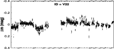
| V22 | PMS/Class iii | CMD | Non-periodic |
| V23 | PMS/Class iii/WTT | CMD | Periodic |
| V24 | PMS/Class iii/WTT | CMD | Periodic |
| V25 | PMS/Class iii | CMD | Non-periodic |
| V26 | MS/field | CMD | Periodic |
| V27 | PMS/Class ii/CTT | IR excess | Non-periodic, large variation in amplitude after 18th Oct 2017 |
| V28 | PMS/Class iii | CMD | Non-periodic |
| V29 | MS/field | CMD | Periodic, Scuti star |
| V30 | MS/field | CMD | Periodic |
| V31 | PMS/Class ii | IR excess | Periodic, relatively longer period 9 days |
| V32 | PMS/Class iii/WTT | CMD | Periodic, large amplitude variation 1.4 mag |
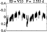
| V33 | PMS/Class iii/WTT | CMD | Periodic |
| V34 | PMS/Class ii | IR excess | Periodic, both intra-night and inter-night variations present in LC |
| V35 | PMS/Class ii/CTT | IR excess | Non-periodic, huge amplitude variation 2 mag |
| V36 | PMS/Class ii/CTT | IR excess | Non-periodic, few brightening events visible in LC |
| V37 | PMS/Class iii/WTT | CMD | Periodic |
| V38 | PMS/Class ii | IR excess | Periodic, relatively longer period 15 days |
| V39 | PMS/Class iii/WTT | CMD | Periodic |
| V40 | MS/field | CMD | Very short period 4 hours |
| V41 | — | — | Non-periodic |
| V42 | — | — | Non-periodic |
| V43 | MS/field | CMD | Non-periodic |
| V44 | MS/field | CMD | Periodic, large variation in amplitude 1.6 mag. |
| V45 | PMS/Class iii/WTT | CMD | Periodic |
| V46 | MS/field | CMD | Non-periodic, large variation in amplitude 1.4 mag. |
| V47 | PMS/Class ii/CTT | IR excess | Non-periodic |
| V48 | MS/field | CMD | Periodic, Lyrae type LC |
| V49 | PMS/Class iii | CMD | Non-periodic |
| V50 | MS/field | CMD | Periodic |
| V51 | MS/field | CMD | Very short period 4 hours |
| V52 | PMS/Class iii | CMD | Non-periodic |
| V53 | PMS/Class ii | IR excess | Periodic, relatively longer period 9 days |
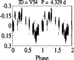
| V54 | PMS/Class ii | IR excess | Periodic |
| V55 | MS/field | CMD | Periodic |
| V56 | MS/field | CMD | Very short period 4 hours |
| V57 | PMS/Class ii | IR excess | Periodic |
| V58 | PMS/Class iii/WTT | CMD | Periodic |
| V59 | MS/field | CMD | Periodic |
| V60 | PMS/Class iii/WTT | CMD | Periodic |
| V61 | MS/field | CMD | Periodic, Lyrae type LC |
| V62 | MS/field | CMD | Periodic |
| V63 | PMS/Class iii | CMD | Non-periodic |
| V64 | MS/field | CMD | Periodic, Lyrae type LC |
| V65 | PMS/Class iii/WTT | CMD | Periodic, very short period 4 hours |
| V66 | — | — | Periodic |
| V67 | PMS/Class iii/WTT | CMD | Periodic |
| V68 | — | — | Periodic |
| V69 | PMS/Class ii | IR excess | Periodic, long period 18 days, amplitude variation 1 mag |
| V70 | PMS/Class iii | CMD | Non-periodic, amplitude variation 1 mag |
| V71 | — | — | Periodic, amplitude variation 1.1 mag |
Appendix A Light curves of the variables not detected in band