Validation tests of Gaussian boson samplers with photon-number resolving detectors

Detectors with photon number resolution implement the normally ordered projection operator [25, 26]

where $:\cdots:$ denotes normal ordering and $c_{j}=0,1,2,3,\dots$ is the number of measured photon counts at the $j$-th detector. Although theoretically there is no upper bound on $c_{j}$, practically PNR detectors saturate for some maximum number of counts $c_{j}^{(\text{max})}$. This value is variable, typically depending on the physical implementation of the detector.

In any multi-mode photon counting experiment, a set of photon count patterns $\boldsymbol{c}=[c_{1},\dots,c_{M}]$ are observed by measuring the output state $\hat{\rho}^{(\text{out})}$. A straightforward extension of Eq.(5) allows one to define the projection operator for a specific count pattern as

For GBS, each pattern is a sample from the full output probability distribution and computing its expectation value corresponds to solving the matrix Hafnian [7, 27]

which is a #P-hard computational task due to its relationship to the matrix permanent. Here, $\text{Haf}(\boldsymbol{B}_{S})$ is the Hafnian of the square sub-matrix of $\boldsymbol{B}=\boldsymbol{U}\left(\bigoplus_{j=1}^{M}\tanh(r_{j})\right)\boldsymbol{U}^{T}$ for pure state inputs with zero displacement, where the sub-matrix is formed from the output channels with recorded photon counts. The symmetric matrix $\boldsymbol{B}$ is related to the kernel matrix $\boldsymbol{A}=\boldsymbol{B}\bigoplus\boldsymbol{B}^{*}$ which is formed from the $2M\times 2M$ covariance matrix $\boldsymbol{Q}$ as [28]

where $\boldsymbol{I}_{M}$ denotes the $M\times M$ identity matrix. When the covariance matrix elements are non-negative, the kernel matrix and hence the symmetric matrix $\boldsymbol{B}$ are also non-negative [28] and the Hafnian can be estimated in polynomial time [29, 30].

In the current generation of GBS networks, photon loss is the dominant noise source. Although there is evidence that sampling from a lossy GBS distribution is also a #P-hard computational task [31], output photons from experiments implementing high loss networks become classical [32], allowing the output distribution to become efficiently sampled. There is currently no clear boundary between the computationally hard and efficiently sampled regimes, but a classical algorithm that exploits large experimental photon loss has recently been developed [33] and shown to produce samples that are closer to the ideal ground truth than recent experiments claiming quantum advantage. The effects of thermalization on the computational complexity of GBS is currently unknown, despite thermalization causing nonclassical photons to become classical at a faster rate than pure losses.

Determining photon counting distributions by binning the photons arriving at photodetectors has a long history in quantum optics. Although binning methods can vary, e.g. binning continuous measurements within a time interval such as inverse bandwidth time [34, 35], such distributions are both experimentally accessible and theoretically useful. For pure squeezed states these can provide evidence of nonclassical behavior, as observed in the even-odd count oscillations [36]. For GBS there is also a statistical purpose, as the set of all possible observable patterns $\mathcal{S}_{P}$ grows exponentially with mode number, causing the output probabilities to become exponentially sparse.

In this paper, we are interested in the total output photon number operator obtained from a subset of $S_{j}$ efficient detectors:

Our observable of interest is then the photon number distribution corresponding to counting the projectors onto eigenstates of $\hat{n}^{\prime}_{S_{j}}$.

Following from the nomenclature introduced in [15], we define the $d$-dimensional grouped photon counting distribution as the probability of observing $\boldsymbol{m}=[m_{1},\dots,m_{d}]$ grouped counts in $j$ distinct subsets of output modes $S_{j}=\{1,\dots,M/d\}$, such that

where $n=\sum_{j=1}^{d}M_{j}\leq M$ is the total correlation order and each grouped count is obtained from the summation $m_{j}=\sum_{i\in S_{j}}c_{i}$. The general form of the pattern projector for any number of output modes within each subset is

Multi-dimensional probabilities are defined over a vector of disjoint subsets $\boldsymbol{S}=\text{$\left(S_{1},\dots,S_{d}\right)$}$ of mode numbers $\boldsymbol{M}=\left(M_{1},\dots,M_{d}\right)$, in which case GCPs become joint probability distributions. This is readily illustrated when $d=2$ and $n=M$, giving $\mathcal{G}_{S_{1},S_{2}}^{(M)}(m_{1},m_{2})$. Increasing the dimension to $d=M$ while keeping the correlation order constant at $n=M$ causes the GCP to converge to the Hafnian.

Therefore, if the correlation order satisfies $n=M$, an increase in GCP dimension corresponds to observing the $d$-th binned Glauber intensity correlation, hence high-order correlations become more statistically significant in the limit $d\rightarrow M$. If such correlations are present in the experimental data, multi-dimensional GCPs provide a more thorough test of quantum advantage as they allow one to directly compare these high-order correlations with their theoretical values [16]. If $n<M$, the GCP becomes a marginal probability as the remaining $M-n$ output modes are ignored.

In its original formulation, Mandel [9, 10] used the normally ordered Glauber-Sudarshan P-representation [11, 12] to evaluate the expectation value in Eq.(10). The P-representation expands the density operator as a diagonal sum of coherent states [11]

hence its commonly called the diagonal P-representation, where $\left|\boldsymbol{\alpha}\right\rangle=\bigotimes_{j=1}^{M}\left|\alpha_{j}\right\rangle$ is a multi-mode coherent state vector with eigenvalues $\boldsymbol{\alpha}=[\alpha_{1},\dots,\alpha_{M}]$ and $P(\boldsymbol{\alpha})$ is the P-representation probability distribution. The diagonal P-representation can be used to evaluate expectation values of the product of normally ordered operators due to the relationship

where $\left\langle\dots\right\rangle$ is a quantum expectation value, $E_{S}$ is an ensemble of random phase-space samples and $\left\langle\dots\right\rangle_{DP}$ is the diagonal-P phase-space ensemble mean.

Following the standard replacement of $\hat{a}_{j}\rightarrow\alpha_{j}$ and $\hat{a}_{j}^{\dagger}\rightarrow\alpha_{j}^{*}$, where $n^{\prime}_{j}=\left|\alpha_{j}\right|^{2}$ and $\hat{n}^{\prime}_{S_{j}}\rightarrow n^{\prime}_{S_{j}}=\sum_{i\in S_{j}}\left|\alpha_{i}\right|^{2}$, Mandel [9, 10] simulates Eq.(10) for $d=1$ and $n=M$ as

where $S=\{1,\dots,M\}$. However, this is only valid for classical states such as coherent, thermal and squashed states [39] as they are defined entirely by their diagonal density matrix elements. Since the density operator of nonclassical states contains off-diagonal elements due to quantum superpositions, if the diagonal P-representation is used for simulations of nonclassical states $P(\boldsymbol{\alpha})$ becomes singular and negative. From standard mathematical requirements that it should be real, normalizable, non-negative and non-singular, it is no longer a probability distribution.

To simulate the photon number distributions of nonclassical states one must instead use the normally ordered positive P-representation [40], which is part of a family of generalized P-representations that produce non-singular and exact phase-space distributions for any quantum state. The positive P-representation expands the density operator as a $4M$-dimensional volume integral [40]

where the additional dimensions allow off-diagonal density matrix elements to be included in the coherent state basis $\left|\boldsymbol{\beta}\right\rangle=\bigotimes_{j=1}^{M}\left|\beta_{j}\right\rangle$ with eigenvalues $\boldsymbol{\beta}=[\beta_{1},\dots,\beta_{M}]$. The coherent amplitudes $\boldsymbol{\alpha}$, $\boldsymbol{\beta}$ are independent and can vary along the entire complex plane. We can also take the real part of Eq.(15), since the density matrix is hermitian. The benefit of using the positive P-representation for photon counting experiments is that it includes the diagonal P-representation when the positive-P distribution satisfies $P(\boldsymbol{\alpha},\boldsymbol{\beta})=P(\boldsymbol{\alpha})\delta(\text{$\boldsymbol{\alpha}$-$\boldsymbol{\beta}$})$. This allows us to define classical phase-space as having $\boldsymbol{\beta}=\boldsymbol{\alpha}$, while a nonclassical phase space requires non-vanishing probability of $\boldsymbol{\beta}\neq\boldsymbol{\alpha}$.

Expectation values of products of normally ordered operators for nonclassical states can now be directly calculated from the moments of the positive-P distribution

where we define $\left\langle\dots\right\rangle_{P}$ as the positive-P ensemble mean and have used the c-number replacements $\hat{a}_{j}\rightarrow\alpha_{j}$ and $\hat{a}_{j}^{\dagger}\rightarrow\beta_{j}^{*}$.

To simulate Eq.(10) for nonclassical states requires replacing the total output photon number Eq.(9) by the phase-space observable

such that the general multidimensional probability distribution is

where $\text{d}\mu\equiv\text{d}\boldsymbol{\alpha}\text{d}\boldsymbol{\beta}$ and the phase-space pattern projector is

We have taken the real part as is required for the applications presented in the next section.

Equation 18 is a more general definition of GCPs than Mandel’s original formulation, since one can now simulate the marginal and multidimensional probabilities of any classical or nonclassical photon counting experiment. To simulate GCPs for input photons in a number state, it is more efficient to use another generalized P-representation: the complex P-representation. In this case $P(\boldsymbol{\alpha},\boldsymbol{\beta})$ includes a complex weight due to expanding the density operator as a contour integral [40]. Although the positive P-representation exists for Fock states, it has larger sampling errors than the complex version [41], meaning fewer stochastic samples are needed to perform accurate simulations.

Unlike methods for threshold detectors [15], Eq.(18) doesn’t require multidimensional inverse discrete Fourier transforms, which increase computation time significantly [16]. Since threshold detector outputs are always binary, the largest number of observable photon counts in a pattern corresponds to a detection event in every output mode, such that $\sum_{i}^{M}c_{i}\leq M$ where the largest observable grouped count is $m^{(M)}$.

Since PNR detectors can resolve multiple photons arriving at each detector, an experiment or classical algorithm replicating photo-detection measurements can now produce count patterns where $\sum_{i}^{M}c_{i}>M$, in which case $m^{(M)}$ is no longer the largest observable grouped count. Instead of scaling with mode number, numerical simulations scale with photon count bins, where we define the maximum observable grouped count as $m^{(\text{max})}$. For experiments with small mean input photon numbers or high losses, one may have $m^{(\text{max})}<m^{(M)}$, while low losses and large photon numbers will produce $m^{(\text{max})}>m^{(M)}$. Typically, we choose $m^{(\text{max})}$ to occur when probabilities are of the order $\mathcal{G}_{S}^{(n)}(m^{(\text{max})})=10^{-7}$ or smaller, providing a standard cutoff for very small probabilities as was implemented in previous methods [15, 16].

Since our observable of interest is the total output photon number Eq.(9), this method requires a photon counting experiment to accurately measure the number of counts arriving at each detector, such that $\left\langle\hat{p}_{j}(c_{j}^{(\text{max})}+1)\right\rangle=0$. Failure to satisfy this requirement would mean output photons in the summations Eq.(9) would be larger than detected counts, leading to inaccurate comparisons. In some regards this is a benefit, as it allows one to determine whether the experimental counts are actually measuring all possible output photons, as some exact algorithms exploit these unmeasured photons to decrease GBS simulation time [20].

Initial coherent amplitudes are generated by randomly sampling the phase-space distribution of a specific state. For most states, analytical forms of this distribution exist, allowing one to derive an analytical expression for the initial samples of each state. Here we simply recall previously derived results for squeezed states [15], so that the theory presented is complete, since the form of the positive-P distribution doesn’t depend on the type of measurement, that is, PNR or not.

For applications to GBS, we first consider the ideal case with pure squeezed state inputs. In order to define the input density operator Eq.(1) in the positive P-representation we first expand each state as an integral over real coherent states [42]

with normalization constant $C_{j}=\sqrt{\gamma_{j}+1}/(\pi\gamma_{j})$ and $\gamma_{j}=\exp(2r_{j})-1$. After some straightforward calculations, the input density operator becomes

where the positive-P distribution for pure squeezed states is [15]

For small $\epsilon$, thermalized squeezed states remain nonclassical and produce a modified output distribution that more closely resembles recent experimental distributions using threshold detectors [15, 16]. Due to this non-classicality, it has been shown [16] that even if an experiments claim of quantum advantage against the ideal distribution becomes invalidated by classical algorithms that replicate photo-detection measurements [18, 19, 16], it may still be able to claim quantum advantage against this non-ideal thermalized distribution.

From this model of decoherence, one can introduce a general random sampling formalism to generate initial stochastic samples for any Gaussian input [15]

where $\left\langle w_{j}w_{k}\right\rangle_{P}=\delta_{jk}$ are real Gaussian noises and the quadrature variances are defined in Eq.(3). For classical inputs, $\sigma_{y_{j}}$ is real and $\alpha_{j}=\beta_{j}$. For quantum inputs, $\sigma_{y_{j}}$ is imaginary and $\alpha_{j}\neq\beta_{j}$. Following from Eq.(4), the output stochastic amplitudes used to perform simulations are then obtained via the transformations $\boldsymbol{\alpha}^{\prime}=\boldsymbol{T}\boldsymbol{\alpha}$ and $\boldsymbol{\beta}^{\prime}=\boldsymbol{T}\boldsymbol{\beta}$ where the amplitudes $\boldsymbol{\alpha}^{\prime}$, $\boldsymbol{\beta}^{\prime}$ correspond to measurements of the density matrix $\hat{\rho}^{\text{(out)}}$.

To test whether Eq.(18) can be utilized to simulate nonclassical photon counting experiments using PNR detectors with perfect squeezers, photodetectors and photonic networks with uniform photon loss, we first simulate small sized GBS networks $M=N=16$ and $M=N=72$ with uniform squeezing $\boldsymbol{r}=[0.89,\dots,0.89]$ and amplitude loss rates $t=0.6$ and $t=0.56$, respectively.

Comparisons between positive-P moments and the exact distribution Eq.(24) are presented in Fig.(1a) and Fig.(1b) for these networks where simulations are performed for an ensemble size of $E_{S}=2.4\times 10^{6}$. In the limit of large $E_{S}$ the positive-P moments converge to moments of a distribution (see Eq.(16)). The exact size of $E_{S}$ required for a given accuracy varies. An ensemble size of the order $E_{S}\geq 10^{6}$ is generally needed for relative errors less than $10^{-3}$, typical of current experimental accuracy.

For both network sizes and loss rates, the positive-P moments converge to the required exact distribution with errors $<10^{-3}$. Increasing the network sizes to $M=N=216$ and $M=N=288$, positive-P moments simulated for loss rates $t=0.57$ and $t=0.6$ are presented in Fig.(1c) and Fig.(1d). In both cases, moments converge to the exact distribution with errors $<10^{-3}$ such that they are not visible in the graphics. Therefore, in the loss regimes of the current experiments, the positive P-representation provides an accurate method to validate experimental networks. For larger sized networks within the ultra-low loss regime this is also true, as the even-odd count oscillations vanish for much smaller amplitude loss rates.

A number of statistical tests have been proposed to validate experimental GBS networks. These include total variation distance [18, 5], cross-entropy measures [18, 19, 33], two and higher-order correlation functions [43, 4], and Bayesian hypothesis testing [4, 39]. Although these tests provide useful insights into the behavior of specific correlations, they are limited to either small size systems or patterns with small numbers of detected photons, as they require computing the probabilities of specific count patterns, which is a #P-hard task.

If these patterns are closer to the ground truth distribution than classical algorithms replicating photo-detection measurements, then its assumed patterns from larger sized systems claiming quantum advantage will also pass these tests. The ground truth distribution is the target distribution GBS aims to sample from when losses are included in the transmission matrix. Generally its assumed to be close to the ideal lossless distribution, although this may not necessarily be the case.

In this work, the primary statistical test used to validate experimental data are chi-square tests [44], which in terms of GCPs are defined as [15]

Here we use the shorthand notation $\mathcal{\bar{G}}_{i}=\left\langle\mathcal{G}_{\boldsymbol{S}}^{(n)}(m_{j_{i}})\right\rangle_{P}=E_{S}^{-1}\sum_{e=1}^{E_{S}}\left(\mathcal{G}_{\boldsymbol{S}}^{(n)}(m_{j_{i}})\right)_{(e)}$ for the stochastic trajectory $e\in E_{S}$ to denote the positive-P GCP ensemble means of the $i=1,2,\dots,k$ photon count bin for the $j=1,\dots,d$ grouped count, which coverages to the true theoretical GCP in the limit $\mathcal{G}_{S,i}=\lim_{E_{S}\rightarrow\infty}\bar{\mathcal{G}}_{S,i}$ for any general input state $S$. Simulated ensemble means are then compared to the experimental GCPs $\mathcal{G}_{E,i}=N_{E}^{-1}\sum_{i}c_{i}$ formed from $N_{E}\subset\mathcal{S}_{P}$ photon count patterns.

Chi-square tests are used for two reasons: the first is that its a standard test applied to data from random number generators [14], where the summation is performed over $k$ count bins satisfying $\sum_{i\in S_{j}}c_{i}>10$. The second is that it contains an explicit dependence on both theoretical and experimental sampling errors as $\sigma_{i}^{2}=\sigma_{E,i}^{2}+\sigma_{T,i}^{2}$, where $\sigma_{E,i}\propto 1/\sqrt{N_{E}}$ is the estimated experimental sampling error. This provides a method of accurately determining whether observed differences are caused by large sampling error, as is the case for sparse data.

Output $\chi^{2}$ values follow a chi-squared distribution that is positively skewed for small $k$. Performing a Wilson-Hilferty transformation [45], which transforms the chi-square result as $\chi^{2}\rightarrow\left(\chi^{2}/k\right)^{1/3}$, the chi-square distribution converges to a Gaussian distribution $\left(\chi^{2}/k\right)^{1/3}\rightarrow\mathcal{N}\left(\mu_{\mathcal{N}},\sigma_{\mathcal{N}}^{2}\right)$ with mean $\mu_{\mathcal{N}}=(9k-2)/9k$ and variance $\sigma_{\mathcal{N}}^{2}=2/(9k)$ for $k\geq 10$ due to the central limit theorem [45, 46]. This allows one to convert chi-square results into measurable probability distances using approximate Z-statistic, or Z-score, tests [47]

which measures how many standard deviations away a test statistic is from its expected normally distributed mean.

The results presented in subsequent subsections use the notation introduced in [16]. Comparisons between theory and experiment for simulations with pure squeezed states input into the experimental $M\times M$ $\boldsymbol{T}$-matrix are denoted by the subscript $EI$, which we call the ideal ground truth distribution. Our ideal ground truth corresponds to the ground truth distributions used in Ref. [5]. However they differ from the non-ideal, or modified, ground truth distribution that includes realistic experimental effects such as thermalization, and measurement corrections in the theoretical simulations, which are denoted by the subscript $ET$.

In all cases, agreement within sampling errors produces test results of $\chi^{2}/k\approx 1$ and $\left|Z\right|\leq 1$ when accounting for stochastic fluctuations in the output statistics. For Z-statistic tests we use a regime of validity with the limit $Z\leq 6$ to define accurate comparisons. Above this limit test statistics are more than $6\sigma_{\mathcal{N}}$ from their predicted means, corresponding to very small observable probabilities.

Due to claims of quantum advantage, in this section we focus predominantly on validating count patterns from the $216$-mode high squeezing (HS) parameter and $288$-mode experimental data sets. Summary tables of chi-square and Z-statistic test results for all Borealis data sets can be found in Appendix A.

First, we compare the theoretical one-dimensional GCPs of the ideal ground truth distribution to the experimental total counts. Similar comparisons were performed in [5], however it was found that at least for the $288$-mode data set the ideal ground truth total count distribution was incorrect [48], leading to inaccurate comparisons. Results of phase-space simulations are presented in Fig.(2a) for the $216$-mode HS data set and Fig.(3a) for the $288$-mode data set. In both cases, the simulated GCP ideal ground truth distributions appear to closely resemble the experimental data. However, upon closer inspection there are significant differences between the two distributions.

This is first observed numerically from statistical testing, where the $216$-mode HS experiment produces a chi-square result of $\chi_{EI}^{2}/k\approx 54$ with $Z_{EI}\approx 70$ and count patterns from the $288$-mode experiment output $\chi_{EI}^{2}/k\approx 411$ with $Z_{EI}\approx 167$. Although both experimental GCPs are far from their pure squeezed state distributions, the $288$-mode distribution is $98\sigma_{\mathcal{N}}$ further from its expected normally distributed mean. These numerical differences are also reflected graphically by plotting the normalized difference between distributions $\Delta\mathcal{G}_{S}^{(M)}(m)/\sigma_{i}=\left(\mathcal{G}_{E,i}-\bar{\mathcal{G}}_{I,i}\right)/\sigma_{i}$, which is plotted in Fig.(2b) for the $216$-mode HS data set and Fig.(3d) for the $288$-mode data set.

Once a thermalization component $\epsilon$ is added to the input states and a transmission matrix measurement correction $t$ is applied as $t\boldsymbol{T}$, the positive-P simulated GCPs agree within sampling error to the experimental distributions. The $216$-mode HS data set requires $\epsilon=0.0510\pm 0.0005$ and $t=0.9941\pm 0.0005$ to output $\chi_{ET}^{2}/k\approx 0.88\pm 0.02$ and $\left|Z_{ET}\right|\approx 1\pm 0.2$, while the best-fit theoretical GCP for $288$-mode data uses a similar thermalization component $\epsilon=0.0547\pm 0.0005$ and measurement correction $t=0.9848\pm 0.0005$ to produce $\chi_{ET}^{2}/k\approx 0.87\pm 0.02$ and $Z_{ET}\approx\left|1.1\right|\pm 0.2$. This exact agreement between theory and experiment is reflected in the normalized difference plots as seen in Fig.(2d) and Fig.(3d) which have noticeably decreased from their pure squeezed state comparisons.

Similar results are obtained for the $72$-mode and $216$-mode low squeezing (LS) experiments. In these cases, comparisons with the ideal ground truth, which output $Z_{EI}=72$ and $Z_{EI}=66$ respectively, converge to a within sampling error agreement with a thermalized theory such that $\left|Z_{ET}\right|\approx 0.2\pm 0.2$ for the $72$-mode experiment and $\left|Z_{ET}\right|\approx 0.89\pm 0.1$ for the $216$-mode LS experiment.

Despite this excellent agreement between theoretical and experimental GCPs once decoherence and measurement corrections are accounted for, we note that stronger validation tests of quantum advantage based on multidimensional GCPs cannot be performed on these data sets. As the dimension increases, the number of bins generated scales as $\left(Md^{-1}+1\right)^{d}$. If there are too few counts per bin, i.e. the bins become more sparse, the experimental sampling errors of these bins increase dramatically, causing statistical tests to become dominated by sampling errors, outputting artificially small results.

Earlier works [16] on recent threshold detector experiments generating $N_{E}\approx 4\rightarrow 5\times 10^{7}$ count patterns showed these sampling error limitations arose for a GCP dimension of $d=4$, such that reliable validation tests could only be performed for $d<4$. However, the majority of data sets from Borealis generate $N_{E}\approx 1\times 10^{6}$ patterns, causing sampling errors to become dominant at only $d=2$, limiting comparisons to only $d=1$.

The exception to this is the $16$-mode experiment whose $N_{E}\approx 8.4\times 10^{7}$ samples were used benchmark the system architecture through total variation distance tests as the system is small enough that output photo-detection measurements can be replicated exactly. Interestingly, the one-dimensional GCP for this data set is further from its ideal ground truth distribution than most experiments performed using the Borealis quantum network, where $\chi_{EI}^{2}/k\approx 2.5\times 10^{3}$ and $Z_{EI}=163$. Unlike data sets claiming quantum advantage, including decoherence and $\boldsymbol{T}$-matrix corrections is no longer enough to obtain a within sampling error agreement between theoretical and experimental GCPs, instead producing statistical test results of $\chi_{ET}^{2}/k\approx 14\pm 2$ and $Z_{ET}\approx 18\pm 1$.

Due to the large number of samples, statistical tests of multi-dimensional GCPs can be performed on this data set. A small increase in the GCP dimension to $d=2$ shows the $16$-mode data is even further from both the ideal and non-ideal ground truth distributions once high-order correlations become more statistically prevalent, outputting $Z_{EI}=301$ and $Z_{ET}=86$. An exponential number of comparison tests can be performed by randomly permuting the measured photon count patters [16], where each permutation allows one to compare different binned correlation moments. As some correlation moments may be closer to their theoretical values than others, Z-scores are likely to vary between permutations, as was observed in threshold detector experiment comparisons [16]. Focusing on comparisons with the non-ideal ground truth, a mean increase in the resulting Z-scores is observed from ten permutations, such that $\left\langle Z_{ET}\right\rangle_{\mathcal{RP}}\approx 139$, where $\left\langle\dots\right\rangle_{\mathcal{RP}}$ denotes a mean over random permutations. Although some permutations are closer to the non-ideal ground truth, with the closest being $Z_{ET}\approx 73$, the majority are further, where the largest observed Z-score was $Z_{ET}\approx 235$ from a single permutation.

Although this is not unexpected, such results indicate further systematic errors besides those tested are present. We conjecture that the presence of further systematic errors other than decoherence and measurement errors are also present in the $216$-mode HS and $288$-mode implementations. However the small sample size means such errors cannot be resolved in statistical testing for these data sets, limiting a thorough analysis.

Finally, for completeness, we simulate the mean output photon number moments $\left\langle\hat{n}^{\prime}_{j}\right\rangle$ for all $j$ modes, where summary tables of statistical test results for all data sets is also presented in Appendix A. As with the GCP comparisons, count patterns from the $216$-mode HS and $288$-mode experiments are far from their theoretical first-order moments for pure squeezed state inputs with $Z_{EI}\approx 86$ and $Z_{EI}\approx 192$ for the $216$-mode HS and $288$-mode data sets respectively.

However, unlike the GCP comparisons, decoherence and transmission matrix corrections no longer cause the theoretical moments to be within error of the experimental moments, where $Z_{ET}\approx 45$ for the $216$-mode HS data set and the $288$-mode data set is $Z_{ET}\sigma_{\mathcal{N}}\approx 63\sigma_{\mathcal{N}}$ standard deviations away from its expected mean. Similar trends are present for all data sets where, as was the case for GCPs, the $16$-mode moments are furthest from their expected first order moments than any other experiment. We emphasize that statistical testing is more accurate for this data set due to the large number of experimental samples, allowing one to resolve finer differences between theoretical and experimental photon number moments.

One noticeable feature in the experimental and theoretical moments is the decrease in $\left\langle\hat{n}^{\prime}_{j}\right\rangle$ as $j\rightarrow M$, with sharp decreases occurring for later modes as seen in Fig.(4) for $175<j<216$ and Fig.(5) for $250<j<288$, while distinct sharp spikes in the moments occur every $16$ modes. This clear structure is present in all data sets from this experiment but is not present in previous implementations with threshold detectors [3, 4] and is likely due to the time-domain multiplexing scheme used to form the linear network in Ref. [5]. The experimental set-up interferes a train of input squeezed photons on multiple fibre delay lines separated by temporal bins of various dimension. Output pulses are then sent into a 1-to-16 mode demultiplexer before measurements are performed by PNR detectors.

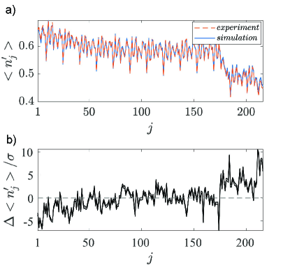
Considering its input-output ratio the demultiplexer may be the cause of the periodic spikes. However the structure in the form of the overall decrease in $\left\langle\hat{n}^{\prime}_{j}\right\rangle$ for increasing mode number may be due to the use of fibre delay lines. Although providing a more compact architecture, it comes at the expense of reduced connectivity, i.e. photon interference between all modes isn’t possible. This has the effect of introducing a structure to the output photons that can be exploited by classical samplers such as the tree-width sampler [49].

Let $Y$ be an i.i.d random variable with probability density function $P(y)$, then the $n$-th raw moment is defined as

Suppose one generates $\mathcal{S}$ samples denoted $y_{1},\dots,y_{\mathcal{S}}$ from the distribution $P(y)$. The $n$-th sample raw moment is then defined as [51, 52, 53]

the expected value of which is an unbiased estimator of $\mu^{\prime}_{n}$

For our purposes, we are interested in the variance $\sigma_{m^{\prime}_{n}}^{2}=\left\langle(m^{\prime}_{n})^{2}\right\rangle-\left\langle m^{\prime}_{n}\right\rangle^{2}$. Following from Ref. [51], the expectation value of the squared moment is simplified as

where the summations have been expanded to include instances of equal $l=i=j$ and non-equal $i\neq j$ samples. Utilizing the simplifications $\sum_{i=1}^{\mathcal{S}}\left\langle y_{i}^{n}\right\rangle=\mathcal{S}\mu^{\prime}_{n}$ from Eq.(32) and $\sum_{i\neq j}^{\mathcal{S}}=\sum_{i}^{\mathcal{S}-1}\sum_{j}^{\mathcal{S}}$, the second-order sample raw moment is simplified as

allowing one to estimate the variance in the sample raw moment as [51]

Its possible to extend the above description for univariate statistics to the multivariate case. Let $\boldsymbol{Y}=[Y_{1},Y_{2},\dots]$ be a vector of i.i.d random variables with multivariate probability density $P(\boldsymbol{y})$, where $\boldsymbol{y}=[y_{1},y_{2},\dots]$. The $n$-th raw moment is then defined as

As in the univariate case, suppose one generates $\mathcal{S}$ samples of the $j=1,2,\dots$-th random variable in $\boldsymbol{Y}$, denoted $y_{1,j},\dots,y_{\mathcal{S},j}$, then the multivariate $n$-th sample raw moment is defined as [52]

whose expected value is an unbiased estimate of the multivariate raw moment [53]

Following from the derivation of the univariate case, the variance of the multivariate raw sample moment is obtained as [54]

By setting $n_{1}=n_{2}=\dots=1$, sampling errors for higher photon number moments such as $\left\langle\hat{n}^{\prime}_{j}\hat{n}^{\prime}_{k}\right\rangle$, $\left\langle\hat{n}^{\prime}_{j}\hat{n}^{\prime}_{k}\hat{n}^{\prime}_{l}\right\rangle$ can now be estimated.

In this paper, the raw moments of interest are the mean output photon numbers per mode $\left\langle\hat{n}^{\prime}_{j}\right\rangle$. Using Eq.(35), the experimental sampling errors can therefore be estimated as

References

- Knill et al. [2001] E. Knill, R. Laflamme, and G. J. Milburn, A scheme for efficient quantum computation with linear optics, Nature 409, 46 (2001).
- Aaronson and Arkhipov [2013] S. Aaronson and A. Arkhipov, The Computational Complexity of Linear Optics, Theory of Computing 9, 143 (2013).
- Zhong et al. [2020] H.-S. Zhong, H. Wang, Y.-H. Deng, M.-C. Chen, L.-C. Peng, Y.-H. Luo, J. Qin, D. Wu, X. Ding, Y. Hu, et al., Quantum computational advantage using photons, Science 370, 1460 (2020).
- Zhong et al. [2021] H.-S. Zhong, Y.-H. Deng, J. Qin, H. Wang, M.-C. Chen, L.-C. Peng, Y.-H. Luo, D. Wu, S.-Q. Gong, H. Su, Y. Hu, P. Hu, X.-Y. Yang, W.-J. Zhang, H. Li, Y. Li, X. Jiang, L. Gan, G. Yang, L. You, Z. Wang, L. Li, N.-L. Liu, J. J. Renema, C.-Y. Lu, and J.-W. Pan, Phase-Programmable Gaussian Boson Sampling Using Stimulated Squeezed Light, Phys. Rev. Lett. 127, 180502 (2021).
- Madsen et al. [2022] L. S. Madsen, F. Laudenbach, M. F. Askarani, F. Rortais, T. Vincent, J. F. F. Bulmer, F. M. Miatto, L. Neuhaus, L. G. Helt, M. J. Collins, A. E. Lita, T. Gerrits, S. W. Nam, V. D. Vaidya, M. Menotti, I. Dhand, Z. Vernon, N. Quesada, and J. Lavoie, Quantum computational advantage with a programmable photonic processor, Nature 606, 75 (2022).
- Deng et al. [2023] Y.-H. Deng, Y.-C. Gu, H.-L. Liu, S.-Q. Gong, H. Su, Z.-J. Zhang, H.-Y. Tang, M.-H. Jia, J.-M. Xu, M.-C. Chen, J. Qin, L.-C. Peng, J. Yan, Y. Hu, J. Huang, H. Li, Y. Li, Y. Chen, X. Jiang, L. Gan, G. Yang, L. You, L. Li, H.-S. Zhong, H. Wang, N.-L. Liu, J. J. Renema, C.-Y. Lu, and J.-W. Pan, Gaussian boson sampling with pseudo-photon-number-resolving detectors and quantum computational advantage, Phys. Rev. Lett. 131, 150601 (2023).
- Hamilton et al. [2017] C. S. Hamilton, R. Kruse, L. Sansoni, S. Barkhofen, C. Silberhorn, and I. Jex, Gaussian boson sampling, Phys. Rev. Lett. 119, 170501 (2017).
- Quesada et al. [2018] N. Quesada, J. M. Arrazola, and N. Killoran, Gaussian boson sampling using threshold detectors, Physical Review A 98, 062322 (2018).
- Mandel and Wolf [1965] L. Mandel and E. Wolf, Coherence Properties of Optical Fields, Rev. Mod. Phys. 37, 231 (1965).
- Mandel and Wolf [1995] L. Mandel and E. Wolf, Optical Coherence and Quantum Optics (Cambridge University Press, Cambridge, 1995).
- Glauber [1963a] R. J. Glauber, Coherent and Incoherent States of the Radiation Field, Phys. Rev. 131, 2766 (1963a).
- Sudarshan [1963] E. C. G. Sudarshan, Equivalence of Semiclassical and Quantum Mechanical Descriptions of Statistical Light Beams, Phys. Rev. Lett. 10, 277 (1963).
- Bassham III et al. [2010] L. E. Bassham III, A. L. Rukhin, J. Soto, J. R. Nechvatal, M. E. Smid, E. B. Barker, S. D. Leigh, M. Levenson, M. Vangel, D. L. Banks, et al., Sp 800-22 rev. 1a. a statistical test suite for random and pseudorandom number generators for cryptographic applications (2010).
- Knuth [2014] D. E. Knuth, Art of computer programming, volume 2: Seminumerical algorithms (Addison-Wesley Professional, 2014).
- Drummond et al. [2022] P. D. Drummond, B. Opanchuk, A. Dellios, and M. D. Reid, Simulating complex networks in phase space: Gaussian boson sampling, Phys. Rev. A 105, 012427 (2022).
- Dellios et al. [2023] A. S. Dellios, B. Opanchuk, M. D. Reid, and P. D. Drummond, Validation tests of gbs quantum computers give evidence for quantum advantage with a decoherent target (2023), arXiv:2211.03480 [quant-ph] .
- Glauber [1963b] R. J. Glauber, The Quantum Theory of Optical Coherence, Phys. Rev. 130, 2529 (1963b).
- Villalonga et al. [2021] B. Villalonga, M. Y. Niu, L. Li, H. Neven, J. C. Platt, V. N. Smelyanskiy, and S. Boixo, Efficient approximation of experimental gaussian boson sampling, arXiv preprint arXiv:2109.11525 (2021).
- Oh et al. [2023] C. Oh, L. Jiang, and B. Fefferman, Spoofing Cross-Entropy Measure in Boson Sampling, Phys. Rev. Lett. 131, 010401 (2023).
- Bulmer et al. [2022] J. F. F. Bulmer, B. A. Bell, R. S. Chadwick, A. E. Jones, D. Moise, A. Rigazzi, J. Thorbecke, U.-U. Haus, T. Van Vaerenbergh, R. B. Patel, I. A. Walmsley, and A. Laing, The boundary for quantum advantage in Gaussian boson sampling, Sci. Adv. 8, eabl9236 (2022).
- Drummond and Reid [2016] P. D. Drummond and M. D. Reid, Coherent states in projected hilbert spaces, Physical Review A 94, 063851 (2016).
- Drummond and Ficek [2004] P. D. Drummond and Z. Ficek, eds., Quantum Squeezing (Springer-Verlag, Berlin, Heidelberg, New York, 2004).
- Shi and Byrnes [2022] J. Shi and T. Byrnes, Effect of partial distinguishability on quantum supremacy in Gaussian Boson sampling, npj Quantum Inf 8, 54 (2022).
- Drummond and Opanchuk [2020] P. D. Drummond and B. Opanchuk, Initial states for quantum field simulations in phase space, Physical Review Research 2, 033304 (2020).
- Walls and Milburn [2008] D. Walls and G. Milburn, Quantum Optics (Springer, 2008).
- Sperling et al. [2012] J. Sperling, W. Vogel, and G. S. Agarwal, True photocounting statistics of multiple on-off detectors, Phys. Rev. A 85, 023820 (2012).
- Kruse et al. [2019] R. Kruse, C. S. Hamilton, L. Sansoni, S. Barkhofen, C. Silberhorn, and I. Jex, Detailed study of gaussian boson sampling, Physical Review A 100, 032326 (2019).
- Quesada and Arrazola [2020] N. Quesada and J. M. Arrazola, Exact simulation of gaussian boson sampling in polynomial space and exponential time, Physical Review Research 2, 023005 (2020).
- Barvinok [1999] A. Barvinok, Polynomial Time Algorithms to Approximate Permanents and Mixed Discriminants Within a Simply Exponential Factor, Random Struct. Alg. 14, 29 (1999).
- Rudelson et al. [2016] M. Rudelson, A. Samorodnitsky, and O. Zeitouni, Hafnians, perfect matchings and Gaussian matrices, Ann. Probab. 44, 10.1214/15-AOP1036 (2016).
- Deshpande et al. [2022] A. Deshpande, A. Mehta, T. Vincent, N. Quesada, M. Hinsche, M. Ioannou, L. Madsen, J. Lavoie, H. Qi, J. Eisert, D. Hangleiter, B. Fefferman, and I. Dhand, Quantum computational advantage via high-dimensional Gaussian boson sampling, Sci. Adv. 8, eabi7894 (2022).
- Qi et al. [2020] H. Qi, D. J. Brod, N. Quesada, and R. García-Patrón, Regimes of classical simulability for noisy gaussian boson sampling, Physical review letters 124, 100502 (2020).
- Oh et al. [2024] C. Oh, M. Liu, Y. Alexeev, B. Fefferman, and L. Jiang, Classical algorithm for simulating experimental gaussian boson sampling, Nature Physics , 1 (2024).
- Huang and Kumar [1989] J. Huang and P. Kumar, Photon-counting statistics of multimode squeezed light, Phys. Rev. A 40, 1670 (1989).
- Zhu and Caves [1990] C. Zhu and C. M. Caves, Photocount distributions for continuous-wave squeezed light, Phys. Rev. A 42, 6794 (1990).
- Mehmet et al. [2010] M. Mehmet, H. Vahlbruch, N. Lastzka, K. Danzmann, and R. Schnabel, Observation of squeezed states with strong photon-number oscillations, Phys. Rev. A 81, 013814 (2010).
- Wigner [1932] E. Wigner, On the Quantum Correction For Thermodynamic Equilibrium, Phys. Rev. 40, 749 (1932).
- Husimi [1940] K. Husimi, Some formal properties of the density matrix, Proc. Phys. Math. Soc. Jpn. 22, 264 (1940).
- Martínez-Cifuentes et al. [2023] J. Martínez-Cifuentes, K. M. Fonseca-Romero, and N. Quesada, Classical models may be a better explanation of the Jiuzhang 1.0 Gaussian Boson Sampler than its targeted squeezed light model, Quantum 7, 1076 (2023).
- Drummond and Gardiner [1980] P. D. Drummond and C. W. Gardiner, Generalised p-representations in quantum optics, Journal of Physics A: Mathematical and General 13, 2353 (1980).
- Opanchuk et al. [2018] B. Opanchuk, L. Rosales-Zárate, M. D. Reid, and P. D. Drummond, Simulating and assessing boson sampling experiments with phase-space representations, Physical Review A 97, 042304 (2018).
- Adam et al. [1994] P. Adam, I. Földesi, and J. Janszky, Complete basis set via straight-line coherent-state superpositions, Physical Review A 49, 1281 (1994).
- Phillips et al. [2019] D. Phillips, M. Walschaers, J. Renema, I. Walmsley, N. Treps, and J. Sperling, Benchmarking of gaussian boson sampling using two-point correlators, Physical Review A 99, 023836 (2019).
- Pearson [1900] K. Pearson, X. on the criterion that a given system of deviations from the probable in the case of a correlated system of variables is such that it can be reasonably supposed to have arisen from random sampling, The London, Edinburgh, and Dublin Philosophical Magazine and Journal of Science 50, 157 (1900).
- Wilson and Hilferty [1931] E. B. Wilson and M. M. Hilferty, The Distribution of Chi-Square, Proc. Natl. Acad. Sci. U.S.A. 17, 684 (1931).
- Johnson [1970] N. L. Johnson, Continuous Univariate Distributions, Houghton Mifflin Series in Statistics (Houghton Mifflin, Boston, 1970).
- Freund and Wilson [2003] R. J. Freund and W. J. Wilson, Statistical Methods (Elsevier, 2003).
- [48] Private communication. Photon counting distribution for the ideal ground truth of the 288-mode data was independently cross-validated. The distribution presented in the Borealis paper is closer to the experimental data than the actual ideal ground truth presented here.
- Oh et al. [2022] C. Oh, Y. Lim, B. Fefferman, and L. Jiang, Classical Simulation of Boson Sampling Based on Graph Structure, Phys. Rev. Lett. 128, 190501 (2022).
- Kloeden and Platen [1992] P. E. Kloeden and E. Platen, Stochastic Differential Equations, in Numerical Solution of Stochastic Differential Equations (Springer Berlin Heidelberg, Berlin, Heidelberg, 1992) pp. 103–160.
- Rao [2009] C. R. Rao, Linear Statistical Inference and Its Applications (John Wiley & Sons, 2009).
- Fisher [1930] R. A. Fisher, Moments and Product Moments of Sampling Distributions, Proceedings of the London Mathematical Society s2-30, 199 (1930).
- McCullagh [2018] P. McCullagh, Tensor Methods in Statistics: Monographs on Statistics and Applied Probability, first edition. ed., CRC Revivals (Chapman and Hall/CRC, Boca Raton, FL, 2018).
- Kendall et al. [1987] M. G. M. G. Kendall, A. Stuart, and J. K. Ord, Kendall’s advanced theory of statistics, 5th ed. (C. Griffin, London, 1987).
- Loudon [1983] R. Loudon, The Quantum Theory of Light, 2nd ed., Oxford Science Publications (Clarendon Press, Oxford, 1983).