Valid and Exact Statistical Inference for Multi-dimensional Multiple Change-Points by Selective Inference
Abstract
In this paper, we study statistical inference of change-points (CPs) in multi-dimensional sequence. In CP detection from a multi-dimensional sequence, it is often desirable not only to detect the location, but also to identify the subset of the components in which the change occurs. Several algorithms have been proposed for such problems, but no valid exact inference method has been established to evaluate the statistical reliability of the detected locations and components. In this study, we propose a method that can guarantee the statistical reliability of both the location and the components of the detected changes. We demonstrate the effectiveness of the proposed method by applying it to the problems of genomic abnormality identification and human behavior analysis.
1 Introduction
In this paper, we consider the multi-dimensional multiple change-point (CP) detection problem (Truong et al., 2018; Sharma et al., 2016; Enikeeva et al., 2019, 2019; Cho, 2016; Horváth and Hušková, 2012; Jirak, 2015; Cho and Fryzlewicz, 2015; Zhang et al., 2010; Vert and Bleakley, 2010; Lévy-Leduc and Roueff, 2009; Bleakley and Vert, 2011). We denote a multi-dimensional sequence dataset by a matrix , where each column is called location and each row is called component. Each location is represented by a -dimensional vector, whereas each component is represented by one-dimensional sequence with the length . We consider the case where changes exist in multiple locations and multiple components. Multi-dimensional multiple CP detection is an important problem in various fields such as computational biology (Takeuchi et al., 2009b) and signal processing (Hammerla et al., 2016).
We focus on the problem of detecting both location and component when there are changes in multiple components at each of the multiple locations. For example, in the field of computational biology, the identification of genome copy-number abnormalities is formulated as a CP detection problem, where it is important to find changes that are commonly observed in multiple patients. This problem can be interpreted as the problem of detecting both the location (genome position of the genome abnormality) and the component (the patients with the genomic abnormality) of multiple CPs.
Our main contribution in this paper is NOT to propose an algorithm for multi-dimensional multiple CP detection, but to develop a method for evaluating the reliability of the detected CPs. Figure 1 shows an example of the problem we consider in this paper. In this paper, we develop a novel method to quantify the statistical reliability of multiple CP locations and components in the form of -values when they are detected by a certain CP detection algorithm. The importance of evaluating the reliability of AI and machine learning (ML) results has been actively discussed in the context of reliable AI/ML — this study can be interpreted as a contribution toward reliable AI/ML.

Reliability evaluation of the detected CPs is inherently difficult. This is because, in most CP detection problems, only a single dataset is given, and the CP detection and evaluation must be done on the same dataset. Therefore, locations and components of the CPs are selected to fit the observed dataset, which suggests that the selection bias must be properly considered. Unlike supervised learning such as regression and classification, it is not possible to use data splitting or cross-validation.
In traditional statistics, reliability evaluation of CPs has been based on asymptotic theory, i.e., the case where (Enikeeva et al., 2019; Cho, 2016; Horváth and Hušková, 2012; Zhang et al., 2010; Jirak, 2015; Harchaoui et al., 2009; Korostelev and Lepski, 2008). The asymptotic theory of CPs is built on various regularity assumptions, such as sufficiently weak sequential correlations, and it has been pointed out that unless these regularity assumptions are met, the evaluation will be inaccurate. Furthermore, the asymptotic theory of CPs is developed in relatively simple problem settings, such as a single CP or one-dimensional sequence, and it cannot be easily extended to a multi-dimensional multiple CP detection problem.
In this paper, we propose a method for valid and exact (non-asymptotic) statistical inference on CPs by utilizing the framework of conditional selective inference (SI), which has recently received much attention in the context of statistical inference on feature selection (Lee et al., 2016; Taylor and Tibshirani, 2015; Fithian et al., 2014; Tibshirani et al., 2016; Loftus and Taylor, 2014, 2015; Suzumura et al., 2017; Terada and Shimodaira, 2019; Yamada et al., 2018b, a; Le Duy and Takeuchi, 2021; Sugiyama et al., 2021). In the past few years, there have been attempts to extend the conditional SI framework into various problems (Lee et al., 2015; Chen and Bien, 2019; Shimodaira and Terada, 2019; Tanizaki et al., 2020; Duy et al., 2020a; Tsukurimichi et al., 2021; Duy and Takeuchi, 2021), and several researchers have started to utilize conditional SI framework to evaluate the reliability of CPs (Umezu and Takeuchi, 2017; Hyun et al., 2018; Jewell, 2020; Duy et al., 2020b). However, to the best of our knowledge, there is no such study for multi-dimensional multiple CPs. Furthermore, if we simply extends the methods of these existing studies to multi-dimensional multiple CP detection problems, it turns out that the power of the inference would be low. Therefore, we propose a new approach based on conditional SI, which is more powerful than the naive extensions of existing approaches.
2 Problem Statement
Dataset and statistical model
Consider a dataset in the form of a multi-dimensional sequence with the length and the dimension . We denote the dataset as where each row is called a component and each column is called a location. The component, denoted as for , is represented as one-dimensional sequence with the length . The location, denoted as for , is represented as a vector with the length . Furthermore, we denote the -dimensional vector obtained by concatenating rows of as where is an operator to transform a matrix into a vector with concatenated rows.
We interpret that the dataset is a random sample from a statistical model
| (1) |
where is the matrix containing the mean values of each element of , is the covariance matrix for representing correlations between components and is the covariance matrix for representing correlations between locations. Here, we do not assume any specific structure for the mean matrix and assume it to be unknown. On the other hand, the covariance matrices and are assumed to be estimable from an independent dataset where it is known that no change points exist.
Detection of locations and components of multiple CPs
We consider the problem of the identifying both the locations and the components of multiple CPs in the dataset when there exist changes in a subset of the components at each of the multiple CP locations. Let be the number of detected CPs. The locations of the detected CPs are denoted as and the subsets of the components where changes present are denoted as where , , is the set of the components in which changes exist at the location . Elements of is denoted as . For notational simplicity, we also define , and , . Given a multi-dimensional sequence dataset , the task is to identify both the locations and the sets of the components . of the detected multiple CPs (see Fig. 1).
As a CP detection method for both locations and components, we employ a method combining dynamic-programming (DP)-based approach (Bellman, 1966; Guthery, 1974; Bai and Perron, 2003; Lavielle, 2005; Rigaill, 2010) and scan-statistic (SS)-based approach (Enikeeva et al., 2019). This CP detection method is formulated as the following optimization problem:
| (2) |
where
| (3a) | ||||
| (3b) | ||||
| (3c) | ||||
| (3d) | ||||
Here, and are hyperparameters which are explained below, is -dimensional binary vector in which the element is if and otherwise, and is a matrix in which vector is arranged diagonally. The CP detection method in (2) is motivated as follows. We employ the scan statistic proposed in (Enikeeva et al., 2019) as the building block, which was introduced for the problem of detecting a single CP from a multi-dimensional sequence111 Double CUMSUM (Cho, 2016) is known as another CP detection method that enables us to select not only the location but also the subset of the components of the change. We focus on the scan-statistic in this study, but conjecture that our SI framework can be applied also to double CUMSUM. . As a criterion for a single CP at the location and the components , the scan statistic is defined as
We extend the scan statistic in various directions in (2). First, we extended the scan statistic to handle multiple CPs, i.e., multiple locations and the corresponding sets of the components . Next, in each component we consider the mean signal difference between the points before and after the CP location , i.e., the mean difference between and . This is to avoid the influence of neighboring CPs when evaluating the statistical reliability of each location and the components . Here, is considered as a hyperparameter Furthermore, the reason why we use instead of in (3a) is that we consider changes to be common among components if it is within the range of rather than defining common changes as the changes at exactly the same location. Here, is also considered as a hyperparameter.
The optimal solution of (2) can be efficiently obtained by using DP and the algorithm for efficient scan-statistic computation described in Enikeeva et al. (2019). The pseudo-code for solving the optimization problem (2) is presented in Algorithms 1 (SortComp and UpdateDP functions are presented in Appendix A).
Statistical Inference on Detected Locations and Components
The main goal of this paper is to develop a valid and exact (non-asymptotic) statistical inference method for detected locations and components of multiple CPs. For each of the detected location and component , , we consider the statistical test with the following null and alternative hypotheses:
| (4a) | ||||
| (4b) | ||||
This test simply concerns whether the averages of points before and after the CP location is equal or not in the component . Note that, throughout the paper, we do NOT assume that the mean of each component is piecewise-constant function, i.e., the proposed statistical inference method in §3 is valid in the sense that the type I error is properly controlled at the specified significance level (e.g., ). While existing statistical inference methods for CPs often require the assumption on the true structure (such as piecewise constantness, piecewise linearity, etc.), the conditional SI framework in this paper enables us to be free from assumptions about the true structure on although the power of the method depend on the unknown structure.
For the statistical test in (4), a reasonable test statistic is the observed mean signal difference
This test statistic can be written as
by defining an -dimensional vector
where is -dimensional binary vector in which the th element is 1 and 0 otherwise, and is -dimensional binary vector in which the element is 1 if and 0 otherwise. In case both the CP location and the CP component are known before looking at data, since follows the multivariate normal distribution in (1), the null distribution of the test statistic also follows a multivariate normal distribution under the null hypothesis (4a). Unfortunately, however, because the CP location and the CP component are actually selected by looking at the observed dataset , it is highly difficult to derive the sampling distribution of the test statistic. In the literature of traditional statistical CP detection, in order to mitigate this difficulty, only simple problem settings, e.g., with a single location or/and a single component, have been studied by relying on asymptotic approximation with or/and . However, these asymptotic approaches are not available for complex problem settings such as (2), and are only applicable when certain regularity assumptions on sequential correlation are satisfied.
Conditional SI
To conduct exact (non-asymptotic) statistical inference on the locations and the components of the detected CPs, we employ conditional SI. The basic idea of conditional SI is to make inferences based on the sampling distribution conditional on the selected hypothesis (Lee et al., 2016; Fithian et al., 2014). Let us denote the set of pairs of location and component of the detected CPs when the dataset is applied to Algorithm 1 as
To apply conditional SI framework into our problem, we consider the following sampling distribution of the test statistic conditional on the selection event that a change is detected at location in the component , i.e.,
Then, for testing the statistical significance of the change, we introduce so-called selective -value , which satisfies the following sampling property
| (5) |
where is the significance level of the statistical test (e.g., )222 Note that a valid -value in a statistical test should satisfies under the null hypothesis so that the probability of the type I error (false positive) coincides with the significance level . . To define the selective -value, with a slight abuse of notation, we make distinction between the random variables and the observed dataset . The selective -value is defined as
| (8) |
where is the nuisance parameter defined as
Note that the selective -values depend on the nuisance component , but the sampling property in (5) is kept satisfied without conditioning on the nuisance event because is independent of the test statistic . The selective confidence interval (CI) for any which satisfies the coverage property conditional on the selection event can be also defined similarly. See Lee et al. (2016) and Fithian et al. (2014) for a more detailed discussion and the proof that the selective -value (8) satisfies the sampling property (5) and how to define selective CIs.
The discussion so far indicates that, if we can compute the conditional probability in (8), we can conduct a valid exact test for each of the detected change at the location in the component for . Most of the existing conditional SI studies consider the case where the hypothesis selection event is represented as an intersection of a set of linear or quadratic inequalities. For example, in the seminal work of conditional SI in Lee et al. (2016), the selective -value and CI computations are conducted by exploiting the fact that the event that some features (and their signs) are selected by Lasso is represented as an intersection of a set of linear inequalities, i.e., the selection event is represented as a polyhedron of sample (data) space. Unfortunately, however, the selection event in (8) is highly complicated and cannot be simply represented an intersection of linear nor quadratic inequalities. We resolve this computational challenge in the next section. Our basic idea is to consider a family of over-conditioning problems such that the computation of the conditional probability of each of the over-conditioning problems can be tractable and then sum them up to obtain the selective -value in (8). This idea is motivated by Liu et al. (2018) and Le Duy and Takeuchi (2021) in which the authors proposed methods to increase the power of conditional SI for Lasso in Lee et al. (2016).
3 Proposed Method
In this section, we propose a method to compute the selective -value in (8). Because we already know that the test statistic follows a normal distribution with the mean and the variance without conditioning, the remaining task is to identify the subspace defined as
| (11) |
Unfortunately, there is no simple way to identify the subspace because it is an inverse problem of the optimization problem in (2). Therefore, we adopt the following strategy:
-
1.
Reformulate the inverse problem (11) as an inverse problem on a line in ;
-
2.
Consider a family of over-conditioning problems by adding additional conditions.
-
3.
Show that the inverse problem for each of the over-conditioning problems considered in step 2 can be solved analytically;
-
4.
Solve a sequence of inverse problems for a sequence of over-conditioning problems along the line considered in step 1.
3.1 Conditional data space on a line
It is easy to see that the condition indicates that is represented as a line in as formally stated in the following lemma.
Lemma 1.
Let
Then,
This lemma indicates that we do not have to consider the inverse problem for -dimensional data space but only to consider an inverse problem for one-dimensional projected data space
This fact has been already implicitly exploited in the seminal conditional SI work in Lee et al. (2016), but explicitly discussed first in Liu et al. (2018). Here, with a slight abuse of notation, is equivalent to .
3.2 Over-conditioning (OC)
Consider all possible sets of triplets of location and component which can be obtained by applying Algorithm 1 to any multivariate sequence dataset . Since the number of such sets are finite, we can represent each of such sets by using an index as . Let us consider
Then, the conditioning event in (8) is written as
Next, let us delve into Algorithm 1 and interpret this algorithm has the following two steps:
-
1.
Given , compute ,
-
2.
Given , compute ,
where the notation indicates that , and in Algorithm 1 depend on the dataset . Consider all possible pairs of tables which can be obtained by applying the above 1st step of Algorithm 1 to any multivariate sequence dataset . Since the number of such pairs is finite, we can represent each of such pairs by using an index as . Let us now write the above step 2 of Algorithm 1 as and consider
Then, the conditioning event in (8) is written as
3.3 Inverse problem for over-conditioning problem
Based on §3.1 and §3.2, we consider the subset of one-dimensional projected dataset on a line for each of the over-conditioning problems:
Lemma 2.
Let us define the following two sets represented as intersections of quadratic inequalities of :
for and . Then, the subset is characterized as
Here, matrices and a scalar require very complex and lengthy definitions (see Appendix B for their complete definitions). Briefly speaking, is a matrix for the sorting operation required to select , while and are a matrix and a scalar for updating the DP tables which are required to select in . The proof of Lemma 2 is presented in Appendix B. Lemma 2 indicates that the subset for each can be characterized by an intersection of quadratic inequalities with respect to and can be obtained analytically.
3.4 Line search
The results in §3.1, §3.2 and §3.3 are summarized as
Our strategy is to identify by repeatedly applying Algorithm 1 to a sequence of datasets within sufficiently wide range of 333 In §4, we set and because the probability mass outside the range is negligibly small. . Because is characterized by an intersection of quadratic inequalities, it is represented either as an empty set, an interval or two intervals in . For simplicity444 The case where is empty set does not appear in the following discussion, and the extension to the case where is represented as two intervals is straightforward. , we consider the case where is represented by an interval and denoted as .
Our method works as follows. Let . By applying Algorithm 1 to the dataset , we obtain such that . It means that for . Therefore, we next consider where is a very small value (e.g., ). Then, we apply Algorithm 1 to the dataset , and obtain such that . We simply repeat this process up to . Finally, we enumerate intervals such that , which enables us to obtain .
Once is computed, remembering that the test-statistic is normally distributed, the selective -value in (8) is computed based on a truncated normal distribution with the truncation region . Specifically,
where is the cumulative distribution function of the truncated normal distribution with the mean , the variance and the truncation region .
3.5 Discussion
In this section, we discuss the power of conditional SI. It is important to note that a conditional SI method is still valid (i.e., the type I error is properly controlled at the significance level ) in the case of over-conditioning (Fithian et al., 2014). In fact, in the early papers on conditional SI (including the seminal paper by Lee et al. (2016)), the computations of selective -values and CIs were made tractable by considering over-conditioning cases. In the past few years, for improving the power of conditional SI, a few methods were proposed to resolve the over-conditioning issue (Liu et al., 2018; Le Duy and Takeuchi, 2021). In Liu et al. (2018), the authors pointed out that the power can be improved by conditioning only on individual features, rather than on the entire subset of features selected by Lasso. In Le Duy and Takeuchi (2021), the authors proposed how to avoid over-conditioning on Lasso conditional SI by interpreting the problem as a search problem on a line in the data space. In this study, we introduce these two ideas into the task of quantifying the statistical reliability of the locations and components of multiple CPs. Specifically, by only considering the locations of points before and after each CP, the statistical reliability of each location can be evaluated independently of other locations, which results in improved power. Furthermore, the approach of searching for matching conditions on a straight line in the data space is inspired by the method proposed in Le Duy and Takeuchi (2021). In the experiments in §4, the SI conditional on the over-condition is denoted as “proposed-OC”, and it is compared with the minimum (i.e., optimal) condition case denoted as “proposed-MC”.
Optimization approaches to solving families of optimization problems parameterized by scalar parameter are called parametric programming or homotopy methods. Parametric programming and homotopy methods are used in statistics and machine learning in the context of regularization path. A regularization path refers to the path of the (optimal) models when the regularization parameter is continuously varied. Regularization paths for various problems and various models have been studied in the literature (Osborne et al., 2000; Hastie et al., 2004; Rosset and Zhu, 2007; Bach et al., 2006; Rosset and Zhu, 2007; Tsuda, 2007; Lee and Scott, 2007; Takeuchi et al., 2009a; Takeuchi and Sugiyama, 2011; Karasuyama and Takeuchi, 2010; Hocking et al., 2011; Karasuyama et al., 2012; Ogawa et al., 2013; Takeuchi et al., 2013). The algorithm described in this section can be interpreted as a parametric optimization problem with respect to (see Lemma 1). In the context of Conditional SI, the parametric optimization problem was first used in the work by Le Duy and Takeuchi (2021), and this work can be interpreted as an application of their ideas to the multi-dimensional change-point detection problem.
4 Experiments
We demonstrate the effectiveness of the proposed method through numerical experiments. In all experiments, we set the significance level at .
4.1 Synthetic Data Experiments
We compared the following four methods:
-
•
Proposed-MC: the proposed method with minimal (optimal) conditioning;
-
•
Proposed-OC: the proposed method with over-conditioning;
-
•
Data splitting (DS): an approach that divides the dataset into odd- and even-numbered locations, and uses one for CP detection and the other for inference;
-
•
Naive: naive inference without considering selection bias;
The goodness of each method was evaluated using false positive rate (FPR), conditional power.
False Positive Rate
FPR is the probability that the null hypothesis will be rejected when it is actually true, i.e., the probability of finding a wrong CPs. In FPR experiments, synthetic data was generated from the normal distribution . We considered the following two covariance matrices for :
-
•
Independence:
-
•
AR(1):
Here, we set and . We considered a setting in which the number of components is fixed with and the sequence length is changed among . Similarly, we considered a setting where the sequence length is fixed with and the number of components is changed among . We generated 1000 samples from , and detected CPs with hyperparameters and . Then, we chose one detected location randomly and tested the changes at all the detected components. Figures 2 and 3 show the results of FPR experiments. Naive method could not control FPR at the significance level. Similarly, since DS is a method that is valid only when each locations are independent each other, FPR could not be controlled in the case of AR(1). On the other hand, the proposed methods (both proposed-MC and proposed-OC) could control FPR at the significance level.
Conditional Power
The power of conditional SI was evaluated by the proportion of correctly identified CP locations and components. We set the mean matrix with as follows:
Synthetic dataset was generated 1000 times from , where and the same covariance structures as in the FPR experiments were considered. In this setting, we detected locations with , and tested all the detected components. Here, proposed-MC and proposed-OC were evaluated by using the following performance measure (Hyun et al., 2018):
In this experiment, we defined that detection is considered to be correct if detected points are within of the true CP locations. Figure 4 shows the result of conditional power experiments. The power of proposed-MC is much greater than that of proposed-OC, indicating that it is crucially important to resolve over-conditioning issues in conditional SI.


4.2 Real data
Here, we compared the performances of the proposed-MC and the naive method on two types of real datasets. Due to the space limitation, we only show parts of the results: the complete results are presented in Appendix C.
Array CGH
Array Comparative Genomic Hybridization (Array CGH) is a molecular biology tool for identifying copy number abnormalities in cancer genomes. We analyzed an Array CGH dataset for malignant lymphoma cancer patients studied in (Takeuchi et al., 2009b). The covariance matrix (both for independent and AR(1) cases) by using Array CGH data for 18 healthy people for which it is reasonable to assume that there are no changes (copy number abnormalities). Figure 5 shows a part of the experimental results. In the naive test, all the detected CP locations and components are declared to be significant results. On the other hand, the proposed-MC suggests that some of the detected locations and components are not really statistically significant.


Human Activity Recognition
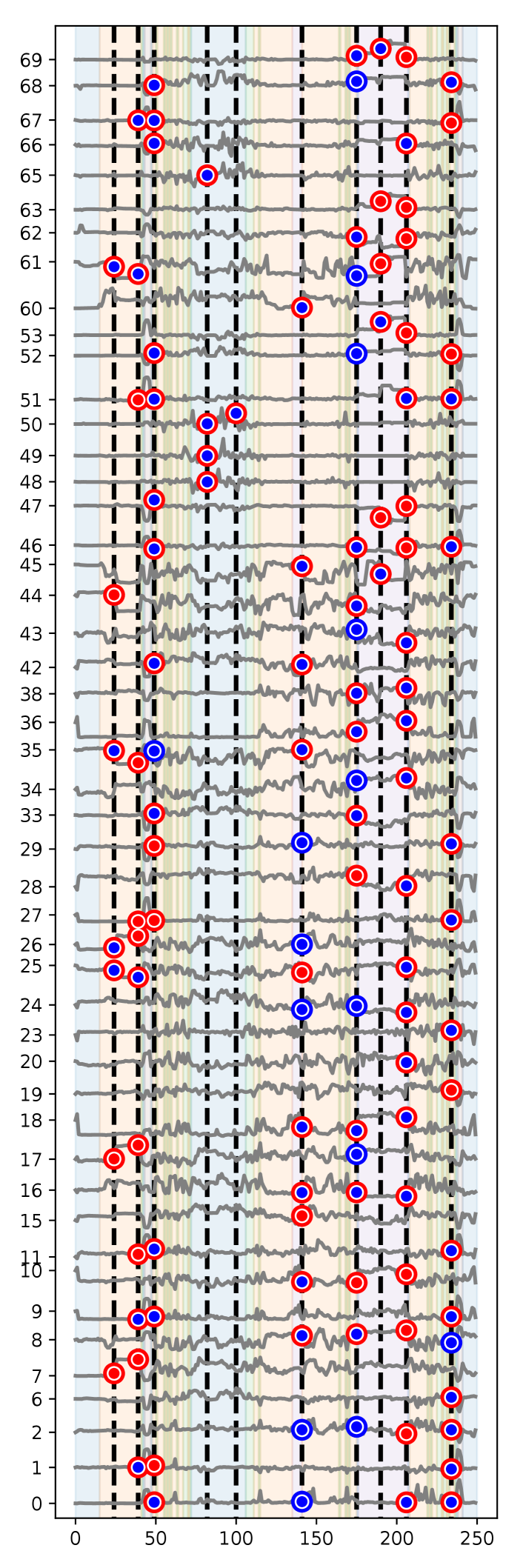
Here, we analyzed human activity recognition dataset studied in (Chavarriaga et al., 2013), in which sensor signals attached in the humber bodies of for subjects were recorded in their daily activities. The sensor signals were recorded at Hz, and locomotion annotations (Stand, Walk, Sit, Lie) and gesture annotations (e.g., Open Door and Close Door) were added manually. We adopted the same preprocessing as (Hammerla et al., 2016) where we used the accelerometers of both arms and back and the IMU data of both feet and signals containing missing values were removed, which resulted in sensor signals. The covariance structures were estimated by using the signals in the longest continuous locomotion state if “Lie” because it indicates the sleeping of the subjects, i.e., no changes exist. In this experiment, the sequence length was compressed to 250 by taking the average so that there is no overlap in the direction of , i.e., the dataset size was and . We used different combinations of hyperparameters . Figure 6 and 7 show parts of the experimental results. The background colors of the figures correspond to the locomotion states, such as blue for None, orange for Stand, green for Walk, red for Sit, and purple for Lie. Most of the detected CP locations and components are declared to be significant by the Naive method. On the other hand, the proposed-MC suggests that some of the detected locations and components are not really statistically significant.


5 Sec5
In this paper, we present a valid exact (non-asymptotic) statistical inference method for testing the statistical significances of CP locations and components. In many applied problems, it is important to identify the locations and components where changes occur. By using the proposed method, it is possible to accurately quantify the reliability of those detected changes.
Acknowledgement
This work was partially supported by Japanese Ministry of Education, Culture, Sports, Science and Technology 16H06538, 17H00758, JST CREST JPMJCR1302, JPMJCR1502, RIKEN Center for Advanced Intelligence Project.
Appendix A Algorithm for UpdateDP, SortComp
In this appendix, we present the pseudo-codes for SortComp and UpdateDP in Algorithm 1.
Appendix B Lemma2
In this appendix, we describe additional details of Lemma 2.
Definition
The matrices , and the scalar in Lemma 2 are defined as follows.
where is an -Dimensional binary vector in which the element is if and otherwise.
Proof
The proof of Lemma 2 is as follows.
Proof.
To prove Lemma 2, it suffices to show that the event that the sorting result at location is as the same as the observed case and the event that the entry of the DP table is as the same as the observed case are both written as intersections of quadratic inequalities of as defined in for and for , , respectively.
First, we prove the claim on the sorting event. Using the matrix defined above, we can write
Therefore, the sorting event is written as
| (12) |
for . By restricting on a line , the range of with which the sorting results are as the same as the observed case is written as
| (13) |
Next, we prove the claim on the DP table. Let
Then, the element of the DP table is written as
Therefore, the DP table event is written as
| (14) |
By restricting on a line , the range of with which the entry of the DP table is as the same as the observed case is written as
| (15) |
Appendix C Additional information about the experiments
In this appendix, we describe the details of the experimental setups and additional experimental results.
C.1 Additional information about experimental setups
We executed all the the experiments on Intel(R) Xeon(R) Gold 6230 CPU 2.10GHz, and Python 3.8.8 was used all through the experiments. The two proposed methods, Proposed-MC and Proposed-OC, are implemented as conditional SIs with the following conditional distributions:
-
•
Proposed-MC: ;
-
•
Proposed-OC: .
C.2 Additional information about synthetic data experiments
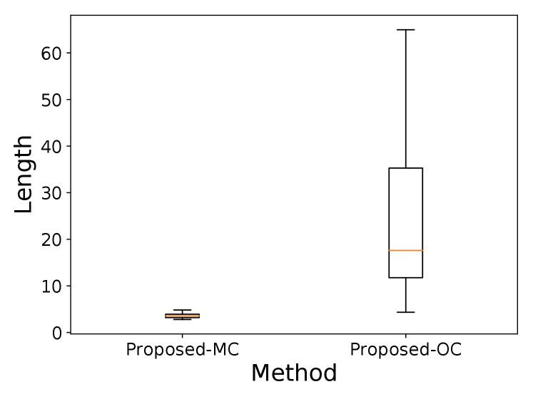
In the synthetic data experiments, in addition to FPR and conditional power, we also compared selective confidence intervals (CI) of Proposed-MC and Proposed-OC. For comparison of selective CIs, we set the mean matrix of the multi-dimensional sequence with as follows:
We considered the same covariance structures as in the experiments for conditional power. For each setting, we generated 100 multi-dimensional sequence samples. Then, the lengths of the 95% CIs in proposed-MC and proposed-OC were compared. Figure 8 shows the result, which are consistent with the results of conditional power555Here, a few outliers are removed for visibility..

C.3 Additional information about real data experiments
Here, we present the detail experimental setups and additional experimental results of the two real data experiments.
Array CGH
We applied the naive method and the proposed-MC method to each of the 22 chromosomes, where and correspond to the length of each chromosome and the number of subjects, respectively. Here, in addition to the result of chromosome 1 in the main paper, we show the results of chromosome 2 – 5 to avoid too large a file size. For the covariance matrix , we considered two alternatives based on the Array CGH data set of 18 healthy subjects, where it is reasonable to assume that CP is not present. The first option is to assume the independence structure and the second option is to assume AR(1) structure. The parameters (for both of independence and AR(1) options), and (for AR(1) option) were estimated as
where . Here, we assumed that correlations between components are uncorrelated because each component represents individual subjects. Figures 9–12 show results of chromosomes 2–5. As we discussed in §4, the naive test declared that most of the detected CP locations and components are statistically significant, whereas the proposed-MC method suggested that some of them are not really statistically significant.


Human Activity Recognition
The original dataset in Chavarriaga et al. (2013) consists of multi-dimensional sensor signals taken from four subjects (S1-S4) in five settings (ADL1-ADL5). In this paper, we applied the naive method and the proposed-MC method only to the first setting (ADL1) of first subject (S1). We considered the same covariance structure options as in the Array CGH data. The covariance structures were estimated by using the signals in the longest continuous locomotion state “Lie” because it indicates the sleeping of the subjects, i.e., no changes exist, as follows:
Here, we used different combinations of hyperparameters . Figures 13–20 show the results of all the parameter settings. As discussed in §4, the naive test declared that most detected CP locations and components are statistically significant, but the proposed-MC method suggested that some of them are not really statistically significant.


References
- Bach et al. [2006] F. R. Bach, D. Heckerman, and E. Horvits. Considering cost asymmetry in learning classifiers. Journal of Machine Learning Research, 7:1713–41, 2006.
- Bai and Perron [2003] Jushan Bai and Pierre Perron. Computation and analysis of multiple structural change models. Journal of applied econometrics, 18(1):1–22, 2003.
- Bellman [1966] Richard Bellman. Dynamic programming. Science, 153(3731):34–37, 1966.
- Bleakley and Vert [2011] Kevin Bleakley and Jean-Philippe Vert. The group fused lasso for multiple change-point detection. arXiv preprint arXiv:1106.4199, 2011.
- Chavarriaga et al. [2013] Ricardo Chavarriaga, Hesam Sagha, Alberto Calatroni, Sundara Tejaswi Digumarti, Gerhard Tröster, José del R Millán, and Daniel Roggen. The opportunity challenge: A benchmark database for on-body sensor-based activity recognition. Pattern Recognition Letters, 34(15):2033–2042, 2013.
- Chen and Bien [2019] Shuxiao Chen and Jacob Bien. Valid inference corrected for outlier removal. Journal of Computational and Graphical Statistics, pages 1–12, 2019.
- Cho [2016] Haeran Cho. Change-point detection in panel data via double cusum statistic. Electronic Journal of Statistics, 10(2):2000–2038, 2016.
- Cho and Fryzlewicz [2015] Haeran Cho and Piotr Fryzlewicz. Multiple-change-point detection for high dimensional time series via sparsified binary segmentation. Journal of the Royal Statistical Society: Series B: Statistical Methodology, pages 475–507, 2015.
- Duy and Takeuchi [2021] Vo Nguyen Le Duy and Ichiro Takeuchi. Exact statistical inference for the wasserstein distance by selective inference. arXiv preprint arXiv:2109.14206, 2021.
- Duy et al. [2020a] Vo Nguyen Le Duy, Shogo Iwazaki, and Ichiro Takeuchi. Quantifying statistical significance of neural network representation-driven hypotheses by selective inference. arXiv preprint arXiv:2010.01823, 2020a.
- Duy et al. [2020b] Vo Nguyen Le Duy, Hiroki Toda, Ryota Sugiyama, and Ichiro Takeuchi. Computing valid p-value for optimal changepoint by selective inference using dynamic programming. In Advances in Neural Information Processing Systems, volume 33, pages 11356–11367, 2020b.
- Enikeeva et al. [2019] Farida Enikeeva, Zaid Harchaoui, et al. High-dimensional change-point detection under sparse alternatives. Annals of Statistics, 47(4):2051–2079, 2019.
- Fithian et al. [2014] William Fithian, Dennis Sun, and Jonathan Taylor. Optimal inference after model selection. arXiv preprint arXiv:1410.2597, 2014.
- Guthery [1974] Scott B Guthery. Partition regression. Journal of the American Statistical Association, 69(348):945–947, 1974.
- Hammerla et al. [2016] Nils Y Hammerla, Shane Halloran, and Thomas Plötz. Deep, convolutional, and recurrent models for human activity recognition using wearables. arXiv preprint arXiv:1604.08880, 2016.
- Harchaoui et al. [2009] Zaid Harchaoui, Félicien Vallet, Alexandre Lung-Yut-Fong, and Olivier Cappé. A regularized kernel-based approach to unsupervised audio segmentation. In 2009 IEEE International Conference on Acoustics, Speech and Signal Processing, pages 1665–1668. IEEE, 2009.
- Hastie et al. [2004] T. Hastie, S. Rosset, R. Tibshirani, and J. Zhu. The entire regularization path for the support vector machine. Journal of Machine Learning Research, 5:1391–415, 2004.
- Hocking et al. [2011] T. Hocking, j. P. Vert, F. Bach, and A. Joulin. Clusterpath: an algorithm for clustering using convex fusion penalties. In Proceedings of the 28th International Conference on Machine Learning, pages 745–752, 2011.
- Horváth and Hušková [2012] Lajos Horváth and Marie Hušková. Change-point detection in panel data. Journal of Time Series Analysis, 33(4):631–648, 2012.
- Hyun et al. [2018] Sangwon Hyun, Kevin Lin, Max G’Sell, and Ryan J Tibshirani. Post-selection inference for changepoint detection algorithms with application to copy number variation data. arXiv preprint arXiv:1812.03644, 2018.
- Jewell [2020] Sean William Jewell. Estimation and Inference in Changepoint Models. University of Washington, 2020.
- Jirak [2015] Moritz Jirak. Uniform change point tests in high dimension. The Annals of Statistics, 43(6):2451–2483, 2015.
- Karasuyama and Takeuchi [2010] M. Karasuyama and I. Takeuchi. Nonlinear regularization path for quadratic loss support vector machines. IEEE Transactions on Neural Networks, 22(10):1613–1625, 2010.
- Karasuyama et al. [2012] M. Karasuyama, N. Harada, M. Sugiyama, and I. Takeuchi. Multi-parametric solution-path algorithm for instance-weighted support vector machines. Machine Learning, 88(3):297–330, 2012.
- Korostelev and Lepski [2008] A Korostelev and O Lepski. On a multi-channel change-point problem. Mathematical Methods of Statistics, 17(3):187–197, 2008.
- Lavielle [2005] Marc Lavielle. Using penalized contrasts for the change-point problem. Signal processing, 85(8):1501–1510, 2005.
- Le Duy and Takeuchi [2021] Vo Nguyen Le Duy and Ichiro Takeuchi. Parametric programming approach for more powerful and general lasso selective inference. In International Conference on Artificial Intelligence and Statistics, pages 901–909. PMLR, 2021.
- Lee and Scott [2007] G. Lee and C. Scott. The one class support vector machine solution path. In Proc. of ICASSP 2007, pages II521–II524, 2007.
- Lee et al. [2015] Jason D Lee, Yuekai Sun, and Jonathan E Taylor. Evaluating the statistical significance of biclusters. Advances in neural information processing systems, 28:1324–1332, 2015.
- Lee et al. [2016] Jason D Lee, Dennis L Sun, Yuekai Sun, Jonathan E Taylor, et al. Exact post-selection inference, with application to the lasso. The Annals of Statistics, 44(3):907–927, 2016.
- Lévy-Leduc and Roueff [2009] Céline Lévy-Leduc and François Roueff. Detection and localization of change-points in high-dimensional network traffic data. The Annals of Applied Statistics, pages 637–662, 2009.
- Liu et al. [2018] Keli Liu, Jelena Markovic, and Robert Tibshirani. More powerful post-selection inference, with application to the lasso. arXiv preprint arXiv:1801.09037, 2018.
- Loftus and Taylor [2014] Joshua R Loftus and Jonathan E Taylor. A significance test for forward stepwise model selection. arXiv preprint arXiv:1405.3920, 2014.
- Loftus and Taylor [2015] Joshua R Loftus and Jonathan E Taylor. Selective inference in regression models with groups of variables. arXiv preprint arXiv:1511.01478, 2015.
- Ogawa et al. [2013] Kohei Ogawa, Motoki Imamura, Ichiro Takeuchi, and Masashi Sugiyama. Infinitesimal annealing for training semi-supervised support vector machines. In International Conference on Machine Learning, pages 897–905, 2013.
- Osborne et al. [2000] Michael R Osborne, Brett Presnell, and Berwin A Turlach. A new approach to variable selection in least squares problems. IMA journal of numerical analysis, 20(3):389–403, 2000.
- Rigaill [2010] Guillem Rigaill. Pruned dynamic programming for optimal multiple change-point detection. arXiv preprint arXiv:1004.0887, 17, 2010.
- Rosset and Zhu [2007] S. Rosset and J. Zhu. Piecewise linear regularized solution paths. Annals of Statistics, 35:1012–1030, 2007.
- Sharma et al. [2016] Shilpy Sharma, David A Swayne, and Charlie Obimbo. Trend analysis and change point techniques: a survey. Energy, Ecology and Environment, 1(3):123–130, 2016.
- Shimodaira and Terada [2019] Hidetoshi Shimodaira and Yoshikazu Terada. Selective inference for testing trees and edges in phylogenetics. Frontiers in Ecology and Evolution, 7:174, 2019.
- Sugiyama et al. [2021] Kazuya Sugiyama, Vo Nguyen Le Duy, and Ichiro Takeuchi. More powerful and general selective inference for stepwise feature selection using homotopy method. In International Conference on Machine Learning, pages 9891–9901. PMLR, 2021.
- Suzumura et al. [2017] Shinya Suzumura, Kazuya Nakagawa, Yuta Umezu, Koji Tsuda, and Ichiro Takeuchi. Selective inference for sparse high-order interaction models. In Proceedings of the 34th International Conference on Machine Learning-Volume 70, pages 3338–3347. JMLR. org, 2017.
- Takeuchi et al. [2009a] I. Takeuchi, K. Nomura, and T. Kanamori. Nonparametric conditional density estimation using piecewise-linear solution path of kernel quantile regression. Neural Computation, 21(2):539–559, 2009a.
- Takeuchi and Sugiyama [2011] Ichiro Takeuchi and Masashi Sugiyama. Target neighbor consistent feature weighting for nearest neighbor classification. In Advances in neural information processing systems, pages 576–584, 2011.
- Takeuchi et al. [2009b] Ichiro Takeuchi, Hiroyuki Tagawa, Akira Tsujikawa, Masao Nakagawa, Miyuki Katayama-Suguro, Ying Guo, and Masao Seto. The potential of copy number gains and losses, detected by array-based comparative genomic hybridization, for computational differential diagnosis of b-cell lymphomas and genetic regions involved in lymphomagenesis. haematologica, 94(1):61, 2009b.
- Takeuchi et al. [2013] Ichiro Takeuchi, Tatsuya Hongo, Masashi Sugiyama, and Shinichi Nakajima. Parametric task learning. Advances in Neural Information Processing Systems, 26:1358–1366, 2013.
- Tanizaki et al. [2020] Kosuke Tanizaki, Noriaki Hashimoto, Yu Inatsu, Hidekata Hontani, and Ichiro Takeuchi. Computing valid p-values for image segmentation by selective inference. 2020.
- Taylor and Tibshirani [2015] Jonathan Taylor and Robert J Tibshirani. Statistical learning and selective inference. Proceedings of the National Academy of Sciences, 112(25):7629–7634, 2015.
- Terada and Shimodaira [2019] Yoshikazu Terada and Hidetoshi Shimodaira. Selective inference after variable selection via multiscale bootstrap. arXiv preprint arXiv:1905.10573, 2019.
- Tibshirani et al. [2016] Ryan J Tibshirani, Jonathan Taylor, Richard Lockhart, and Robert Tibshirani. Exact post-selection inference for sequential regression procedures. Journal of the American Statistical Association, 111(514):600–620, 2016.
- Truong et al. [2018] Charles Truong, Laurent Oudre, and Nicolas Vayatis. A review of change point detection methods. 2018.
- Tsuda [2007] K. Tsuda. Entire regularization paths for graph data. In In Proc. of ICML 2007, pages 919–925, 2007.
- Tsukurimichi et al. [2021] Toshiaki Tsukurimichi, Yu Inatsu, Vo Nguyen Le Duy, and Ichiro Takeuchi. Conditional selective inference for robust regression and outlier detection using piecewise-linear homotopy continuation. arXiv preprint arXiv:2104.10840, 2021.
- Umezu and Takeuchi [2017] Yuta Umezu and Ichiro Takeuchi. Selective inference for change point detection in multi-dimensional sequences. arXiv preprint arXiv:1706.00514, 2017.
- Vert and Bleakley [2010] Jean-Philippe Vert and Kevin Bleakley. Fast detection of multiple change-points shared by many signals using group lars. Advances in neural information processing systems, 23:2343–2351, 2010.
- Yamada et al. [2018a] Makoto Yamada, Yuta Umezu, Kenji Fukumizu, and Ichiro Takeuchi. Post selection inference with kernels. In International Conference on Artificial Intelligence and Statistics, pages 152–160. PMLR, 2018a.
- Yamada et al. [2018b] Makoto Yamada, Denny Wu, Yao-Hung Hubert Tsai, Ichiro Takeuchi, Ruslan Salakhutdinov, and Kenji Fukumizu. Post selection inference with incomplete maximum mean discrepancy estimator. arXiv preprint arXiv:1802.06226, 2018b.
- Zhang et al. [2010] Nancy R Zhang, David O Siegmund, Hanlee Ji, and Jun Z Li. Detecting simultaneous changepoints in multiple sequences. Biometrika, 97(3):631–645, 2010.