Using Quantum Computers to Speed Up Dynamic Testing of Software

It is theoretically possible to convert any CC program into a QC program (because QC implements a quantum Turing machine [7, 3]), but there are limitations and practical considerations (see Section 4). Essentially, a classical algorithm is converted into reversible circuits [20], which are then converted into quantum circuits [9]. These conversions can be done automatically.

Several nascent tools for converting classical to quantum circuits already exist. Qiskit, for example, allows compiling a classical function to a quantum circuit transparently (by adding the decorator @classical_function). Qiskit converts classical circuits to quantum circuits using the Tweedledum library [28]. Currently, the compilation is limited to binary inputs/outputs and logical operators (see Section 3.1.1 for an example). Another example is the staq toolkit, which can convert classical Verilog circuits to a quantum assembly language (QASM) [6]. Finally, StaffCC compiler [18] extension RKQC [16] is also capable of compiling classical circuits to QASM (including integer addition and multiplication operations [34]).

Hopefully, the abovementioned tools will evolve in the future to enable the conversion of any classical program.

Section 2.1 discussed the possibility of interpreting input $x$ into $f$ as a bit string. Furthermore, bit strings can represent arbitrary complex data structures. Thus, to convert $\vec{z}$ into $x$, we must convert $\vec{z}$ into a bit string.

For example, imagine that $\vec{z}$ has two elements: an integer $z_{1}$ and a 3-character string $z_{2}$, i.e., $g(\vec{z})=g(z_{1},z_{2})$. Furthermore, suppose that storing an integer and a string character requires $64$ and $8$ bits, respectively. We will need $88=64+3\times 8$ bits to represent the input, i.e., $N=2^{88}$.

Software programs may produce any output (or no output at all), whereas $f(x)$ should return either zero or one. We can satisfy this requirement by wrapping³³3We can also leverage try-catch blocks in high-level programming languages. $g(\vec{z})$ in code that returns an exit code of $0$ on success and $1$ on error (similar to operating system exit status codes).

Suppose we implement a function $g(z_{1},z_{2})$, where $z_{1}$ is a 2-bit integer and $z_{2}$ is a boolean variable. The next step is to test our implementation of $g(z_{1},z_{2})$.

Suppose we inject two defects, e.g., $g(z_{1},z_{2})$ returns incorrect results when $z_{1}=3$ and $z_{2}=\textrm{false}$ or when $z_{1}=2$ and $z_{2}=\textrm{true}$. Algorithm 3 gives a trivial example of such code. Code review of Algorithm 3 immediately reveals the problem. Of course, in real-world scenarios, we would not know these values of $\vec{z}$ upfront; this simplification is for demonstration purposes only.

Step 2 of Algorithm 2 converts $g(z_{1},z_{2})$ into $f(x)$. As $z_{1}$ and $z_{2}$ can be represented by 3-bit strings, $N=2^{3}=8$. The first two bits of the bit string store an integer $z_{1}$, while the last bit stores a boolean variable $z_{2}$.

We will implement our example using Qiskit; code listing can be found on Zenodo [21].

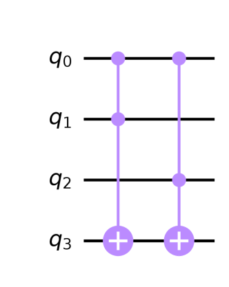
As was described in Section 2.3, converters from a classical to a quantum circuit are still in their infancy, and Qiskit operates only on binary variables. Thus, we must manually reduce the code in Algorithm 3 to the format understood by Qiskit (eventually, converters and compilers will do this automatically). Listing 1 shows the result of the conversion to $f(x)$. Once in this form, Qiskit’s @classical_function decorator automatically converts $f(x)$ to the quantum circuit (so-called bit-flip oracle [25]) shown in Figure 3.

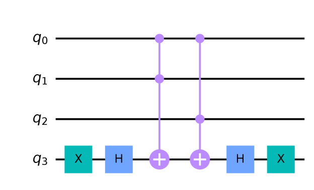
Using Grover’s algorithm requires a phase-flip oracle [25]. Bit-flip oracles are converted to phase-flip oracles by placing their return values between NOT and Hadamard gates as shown in Listing 2. The phase-flip oracle circuit, which we pass to the search algorithm, is shown in Figure 4.

In Step 2 of Algorithm 2, we pass the oracle’s circuit to the quantum counting algorithm⁴⁴4Qiskit’s implementation of the quantum counting algorithm [11] is illustrated in [5, Sec. 3.9]., which returns $K$, the number of inputs causing defects. In our case, $K=2$. As $K\neq 0$ and $K\neq N$, we go to Step 2.

Step 2 of Algorithm 2 involves passing oracle’s circuit to Grover’s algorithm to find specific input values that cause failures. Using the $K$ value from Step 2, we can calculate the number of iterations of Grovers’ algorithm: $r(N,K)=r(8,2)=2$.

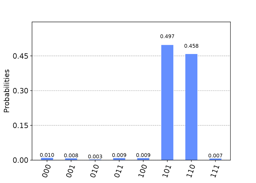
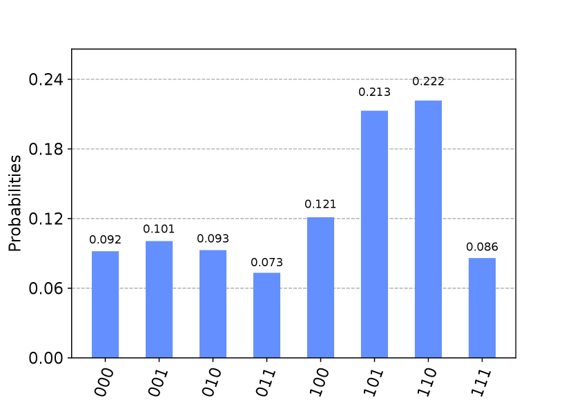
Execution is performed on the Qiskit v.0.37.0 Aer simulator v.0.10.4 (providing an ideal noise-free QC) as well as on the IBM Quantum r4T Processor v.1.0.38 with five qubits, namely, ibmq_lima [2]. With ibmq_lima, we compare the output based on Qiskit’s simulator of ibmq_lima as well as the output from the actual QC.

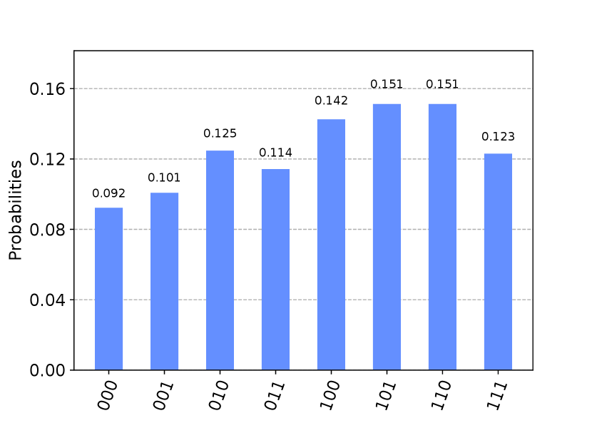
The output of Grover’s algorithm can be seen in Figure 5. According to the simulators and the real QC, 110 and 101 are the top-two returned values of $\omega$. However, due to noise, the $p$-values on the real QC are lower than those on the simulators.

Step 2 of Algorithm 2 converts $\omega$ back to $\vec{z}$ values:

These are the values we expected. In other words, Algorithm 2 correctly identified two inputs that caused errors in software under test.

How laborious is Algorithm 2?

In Step 2, code written in a high-level language (e.g., C/C++ or Python) is compiled into a quantum circuit. Depending on the compiler, the complexity of this process may vary, but compiler designers are aiming for $O(\alpha^{2})$, where $\alpha$ is the size of the input [13]. In practice, even for large code bases with millions of lines of code, compilation on modern CC is relatively fast.

The computation complexity of Steps 2 and 2 is $O(\varepsilon^{-1}\sqrt{N/K})$ and $O(\sqrt{N/K})$, respectively [10, 11]. Complexity of Step 2 is proportional to the number of bits required to represent $x$, i.e., $O(\log_{2}{N})$. Therefore, we estimate that the majority of time will be spent on Steps 2 and 2, with the dominant term $O(\varepsilon^{-1}\sqrt{N/K})$.

When comparing exhaustive testing on CC and QC, QC is faster because exhaustive search on a CC requires $O(N)=O(2^{n})$ computations, while on a QC — only $O(\varepsilon^{-1}\sqrt{N/K})=O(\varepsilon^{-1}2^{n/2}K^{-1/2})$ computations.

$2^{n/2}$ grows much slower⁵⁵5For example, suppose $n=64$ bits. Then $2^{n}=2^{64}\approx 2\times 10^{19}$, while $2^{n/2}=2^{32}\approx 4\times 10^{9}$. than $2^{n}$, but it still increases exponentially. Thus, if our software has input parameters requiring many bits, the search will become prohibitively expensive, even on a QC. Therefore, let us explore non-exhaustive testing methods.

Let us consider the function $g(z_{3})$, where $z_{3}$ is a $64$-bit integer, i.e., $n=64$). There are only three input values we want to test, e.g., $z_{3}=\{7,200,1005\}$.

We will refer to the number of inputs in a subset as $N_{s}$. In our example $N_{s}=3$. To represent the input, we only need $\lceil\log_{2}{N_{s}}\rceil=\lceil\log_{2}{3}\rceil=2$ qubits rather than $64$ qubits. During compilation, we would add a data structure that mapped each of these three values to their 64-bit representations (note that we will still need $64$ auxiliary qubits to build oracle’s circuit, but we will only be measuring the two input qubits).

We will get $O(\varepsilon^{-1}\sqrt{N_{s}/K})=O(\varepsilon^{-1}2^{n_{s}/2}K^{-1/2})$ computations, where $N_{s}=2^{n_{s}}$, if we apply the complexity analysis logic discussed in Section 3.1.2. Therefore, as long as $N\gg N_{s}$, the non-exhaustive test will be significantly faster than the exhaustive test. Moreover, non-exhaustive testing on a CC would require $O(N_{s})=O(2^{n_{s}})$ computations, so QC will outperform CC.

As we need to add the code to map $\vec{z}$ to $x$, the cost of executing the oracle increases compared to the exhaustive testing case. Nevertheless, such look-up tables can be constructed efficiently; e.g., a hash table’s search complexity is $O(1)$. As a result, the computation time increase will be minimal.

References

- [1]
- ibm [2022] 2022. IBM Quantum. https://quantum-computing.ibm.com
- Aaronson [2005] Scott Aaronson. 2005. Quantum computing, postselection, and probabilistic polynomial-time. Proceedings of the Royal Society A: Mathematical, Physical and Engineering Sciences 461, 2063 (2005), 3473–3482.
- Aaronson and Rall [2020] Scott Aaronson and Patrick Rall. 2020. Quantum approximate counting, simplified. In Symposium on Simplicity in Algorithms. SIAM, 24–32.
- Abbas et al. [2020] Amira Abbas, Stina Andersson, Abraham Asfaw, Antonio Corcoles, Luciano Bello, Yael Ben-Haim, Mehdi Bozzo-Rey, Sergey Bravyi, Nicholas Bronn, Lauren Capelluto, Almudena Carrera Vazquez, Jack Ceroni, Richard Chen, Albert Frisch, Jay Gambetta, Shelly Garion, Leron Gil, Salvador De La Puente Gonzalez, Francis Harkins, Takashi Imamichi, Pavan Jayasinha, Hwajung Kang, Amir h. Karamlou, Robert Loredo, David McKay, Alberto Maldonado, Antonio Macaluso, Antonio Mezzacapo, Zlatko Minev, Ramis Movassagh, Giacomo Nannicini, Paul Nation, Anna Phan, Marco Pistoia, Arthur Rattew, Joachim Schaefer, Javad Shabani, John Smolin, John Stenger, Kristan Temme, Madeleine Tod, Ellinor Wanzambi, Stephen Wood, and James Wootton. 2020. Learn Quantum Computation Using Qiskit. http://community.qiskit.org/textbook
- Amy and Gheorghiu [2020] Matthew Amy and Vlad Gheorghiu. 2020. staq—A full-stack quantum processing toolkit. Quantum Science and Technology 5, 3 (2020), 034016.
- Benioff [1980] Paul Benioff. 1980. The computer as a physical system: A microscopic quantum mechanical Hamiltonian model of computers as represented by Turing machines. Journal of statistical physics 22, 5 (1980), 563–591.
- Bennett et al. [1997] Charles H Bennett, Ethan Bernstein, Gilles Brassard, and Umesh Vazirani. 1997. Strengths and weaknesses of quantum computing. SIAM journal on Computing 26, 5 (1997), 1510–1523.
- Bojić [2014] Alan Bojić. 2014. An approach to source code conversion of classical programming languages into source code of quantum programming languages. Journal of Information and Organizational Sciences 38, 2 (2014), 75–82.
- Boyer et al. [1998] Michel Boyer, Gilles Brassard, Peter Høyer, and Alain Tapp. 1998. Tight bounds on quantum searching. Fortschritte der Physik: Progress of Physics 46, 4-5 (1998), 493–505.
- Brassard et al. [1998] Gilles Brassard, Peter Høyer, and Alain Tapp. 1998. Quantum counting. In International Colloquium on Automata, Languages, and Programming. Springer, 820–831.
- Chao and Reichardt [2018] Rui Chao and Ben W Reichardt. 2018. Fault-tolerant quantum computation with few qubits. npj Quantum Information 4, 1 (2018), 1–8.
- Cooper and Torczon [2011] Keith D Cooper and Linda Torczon. 2011. Engineering a compiler (2 ed.). Elsevier.
- Ferrante and Saltalamacchia [2014] Marco Ferrante and Monica Saltalamacchia. 2014. The coupon collector’s problem. Materials matemàtics (2014), 1–35.
- Grover [1996] Lov K Grover. 1996. A fast quantum mechanical algorithm for database search. In 28th annual ACM symposium on theory of computing. ACM, 212–219.
- Holmes [2016] Adam Holmes. 2016. epiqc/RKQC: RKQC is a compiler for reversible logic circuitry. https://github.com/epiqc/RKQC
- Hynninen et al. [2018] Timo Hynninen, Jussi Kasurinen, Antti Knutas, and Ossi Taipale. 2018. Software testing: Survey of the industry practices. In 41st International Convention on Information and Communication Technology, Electronics and Microelectronics (MIPRO). IEEE, 1449–1454.
- JavadiAbhari et al. [2014] Ali JavadiAbhari, Shruti Patil, Daniel Kudrow, Jeff Heckey, Alexey Lvov, Frederic T Chong, and Margaret Martonosi. 2014. ScaffCC: A framework for compilation and analysis of quantum computing programs. In 11th ACM Conference on Computing Frontiers. ACM, 1–10.
- Kuhn et al. [2004] D Richard Kuhn, Dolores R Wallace, and Albert M Gallo. 2004. Software fault interactions and implications for software testing. IEEE trans. on softw. eng. 30, 6 (2004), 418–421.
- Miller et al. [2003] D Michael Miller, Dmitri Maslov, and Gerhard W Dueck. 2003. A transformation based algorithm for reversible logic synthesis. In Design automation conference. IEEE, 318–323.
- Miranskyy [2022] Andriy Miranskyy. 2022. Supplementary material: code listing. https://doi.org/10.5281/zenodo.7065888
- Miranskyy et al. [2022] Andriy Miranskyy, Mushahid Khan, Jean Paul Latyr Faye, and Udson C Mendes. 2022. Quantum Computing for Software Engineering: Prospects. arXiv preprint arXiv:2203.03575 (2022). To appear in Proceedings of the 1st International Workshop on Quantum Programming for Software Engineering.
- Miranskyy and Zhang [2019] Andriy Miranskyy and Lei Zhang. 2019. On testing quantum programs. In 41st Int. Conf. on Softw. Eng.: New Ideas and Emerging Results (ICSE-NIER). IEEE, 57–60.
- Miranskyy et al. [2021] Andriy Miranskyy, Lei Zhang, and Javad Doliskani. 2021. On testing and debugging quantum software. arXiv preprint arXiv:2103.09172 (2021).
- Nielsen and Chuang [2010] Michael A. Nielsen and Isaac L. Chuang. 2010. Quantum Computation and Quantum Information: 10th Anniversary Edition. Cambridge Univ. Press.
- Osherove [2013] Roy Osherove. 2013. The Art of Unit Testing: with examples in C# (2 ed.). Manning.
- Pressman and Maxim [2015] Roger S Pressman and Bruce R. Maxim. 2015. Software engineering: a practitioner’s approach (8 ed.). McGraw Hill.
- Schmitt and De Micheli [2022] Bruno Schmitt and Giovanni De Micheli. 2022. tweedledum: a compiler companion for quantum computing. In 2022 Design, Automation & Test in Europe Conference & Exhibition (DATE). IEEE, 7–12.
- Seidel et al. [2021] Raphael Seidel, Colin Kai-Uwe Becker, Sebastian Bock, Nikolay Tcholtchev, Ilie-Daniel Gheorge-Pop, and Manfred Hauswirth. 2021. Automatic Generation of Grover Quantum Oracles for Arbitrary Data Structures. arXiv preprint arXiv:2110.07545 (2021).
- Sevilla and Riedel [2020] Jaime Sevilla and C Jess Riedel. 2020. Forecasting timelines of quantum computing. arXiv preprint arXiv:2009.05045 (2020).
- Shor [1994] Peter W Shor. 1994. Algorithms for quantum computation: discrete logarithms and factoring. In 35th annual symp. on foundations of comp. sci. IEEE, 124–134.
- Viamontes et al. [2005] George F Viamontes, Igor L Markov, and John P Hayes. 2005. Is quantum search practical? Computing in science & engineering 7, 3 (2005), 62–70.
- Wack et al. [2021] Andrew Wack, Hanhee Paik, Ali Javadi-Abhari, Petar Jurcevic, Ismael Faro, Jay M. Gambetta, and Blake R. Johnson. 2021. Scale, Quality, and Speed: three key attributes to measure the performance of near-term quantum computers. arXiv preprint arXiv:2110.14108 (2021).
- Wang et al. [2016] Feng Wang, Mingxing Luo, Huiran Li, Zhiguo Qu, and Xiaojun Wang. 2016. Improved quantum ripple-carry addition circuit. Science China Information Sciences 59, 4 (2016), 1–8.
- Zomorodi-Moghadam et al. [2014] Mariam Zomorodi-Moghadam, Mohammad-Amin Taherkhani, and Keivan Navi. 2014. Synthesis and optimization by quantum circuit description language. In Transactions on Computational Science XXIV. Springer, 74–91.