Using gravitational waves to see the first second of the Universe

Rishav Roshan and Graham White School of Physics and Astronomy, University of Southampton,
Southampton SO17 1BJ, United Kingdom

Abstract

Gravitational waves are a unique probe of the early Universe, as the Universe is transparent to gravitational radiation right back to the end of inflation. In this article, we summarise detection prospects and the wide scope of primordial events that could lead to a detectable stochastic gravitational wave background. Any such background would shed light on what lies beyond the Standard Model, sometimes at remarkably high scales. We overview the range of strategies for detecting a stochastic gravitational wave background before delving deep into three major primordial events that can source such a background. Finally, we summarize the landscape of other sources of primordial backgrounds.

I Introduction

Gravitational waves (GW) are one of the most striking predictions of Einstein’s theory of general relativity Einstein (1916, 1918). Remarkably, the concept of gravitational waves predates Einstein, as physicists at the turn of the 19th century wondered if there was a gravitational analog of electromagnetic waves Poincaré (1913). Moreover, Einstein famously published an incorrect proof that gravitational waves do not exist Kennefick (2007).¹¹1This was in a paper that was originally rejected by physical review, with the referee later vindicated that Einstein made the mistake of making a pathological coordinate transformation Blum (2022). Eventually, Einstein published a corrected version that argued for the existence of cylindrical gravitational waves Einstein and Rosen (1937). Even still, the recent discovery of gravitational waves by aLIGO Abbott et al. (2016b) is widely seen as one of his greatest triumphs.

Decades before it became possible to observe the Universe via gravitational waves, another consequence of Einstein’s theory was being explored - that the Universe expanded from a hot dense initial state in a theory later coined the “big bang theory” Lemaître (1931). The Big Bang theory predicts that the Universe should expand and cool until the point at which free protons and electrons combine into the first hydrogen atoms, after which the mean free path of photons rapidly grows to the point where its light is visible today in a black body spectrum. This cosmic microwave background radiation (CMB), was later seen in 1964, falsifying the steady state theory and verifying the Big Bang theory of cosmology Penzias and Wilson (1979). Since then we have entered the era of precision measurements of nature’s first light, which allows us to probe features of the primordial fireball Aghanim et al. (2020a). In particular, we can measure the expansion of the Universe and the asymmetry between matter and anti-matterRiotto (1998); Riotto and Trodden (1999); Dine and Kusenko (2003); Cline (2006); Canetti et al. (2012); Morrissey and Ramsey-Musolf (2012); Balazs (2014); White (2016); Bodeker and Buchmuller (2021) at the time when the CMB forms. We have an alternative measurement of these two observables. About a second after the moment of creation, the first nucleons were synthesized and we can cross-check the primordial abundances of hydrogen, helium, and deuterium with our predictions, the latter of which are sensitive to the precise value of the baryon asymmetry and the expansion rate of the Universe Cyburt et al. (2016). In other words, we can calculate the expansion rate and baryon asymmetry during Big Bang nucleosynthesis (BBN) by measuring the primordial abundances. Remarkably, in a triumph of modern cosmology, we find concordance between the cosmic microwave background and Big Bang nucleosynthesis Eidelman et al. (2004); Aghanim et al. (2020a).

Despite the success of our current model of cosmology (up to some recent tensions with data Di Valentino et al. (2021)), physicists face a huge “gap problem” where we know nothing about the period between a early epoch of rapid expansion, known as inflation and BBN. Measured in SI units, the problem does not seem alarming - we are in the dark by a mere second of our history. Measured in terms of temperature demotes cosmology to being a field in its infancy. The history of the Universe potentially spans twenty-two orders of magnitude in temperature between the end of inflation and the onset of BBN de Salas et al. (2015); Delle Rose et al. (2016). Being ignorant of this period renders us incapable of understanding why there is more matter than antimatter Riotto (1998); Riotto and Trodden (1999); Dine and Kusenko (2003); Cline (2006); Canetti et al. (2012); Morrissey and Ramsey-Musolf (2012); Balazs (2014); White (2016); Bodeker and Buchmuller (2021), what dark matter is and how it came to be Bergström (2000); Bertone et al. (2005); Feng (2010); Garrett and Duda (2011); Peter (2012); Bertone and Hooper (2018); Arun et al. (2017); Bertone and Tait (2018); Arbey and Mahmoudi (2021), how hot the Universe was and how did it become so hot after inflation Bassett et al. (2006); Allahverdi et al. (2010), was this period always dominated by radiation or were there early periods of matter domination Allahverdi et al. (2020), was it always in thermal equilibrium or did the Universe come to boil Linde (1979); Grojean and Servant (2007); Boyanovsky et al. (2006); Weir (2018); Mazumdar and White (2019); Caprini et al. (2020a)?

Gravitational wave cosmology is the unrivaled method to make progress on the gap problem - the Universe is transparent to gravitational waves right up to the instant of its birth. Any violent event in that first second will leave a trace in the stochastic gravitational wave background (SGWB) which we can hope to detect today. The next generation promises to birth a new dawn of gravitational wave detection, with ground and space-based interferometers pledging to search for primordial spectra in the $\mu$ Hz to kHz range Aasi et al. (2015); Abbott et al. (2016a); Buikema et al. (2020); Tse et al. (2019); Acernese et al. (2015, 2019); Akutsu et al. (2019); Aso et al. (2013); Reitze et al. (2019); Amaro-Seoane et al. (2017); Sesana et al. (2021); Kawamura (2019) whereas astrometry Kaiser and Jaffe (1997); Brown et al. (2018); Boehm et al. (2017); Book and Flanagan (2011); Moore et al. (2017); Mihaylov et al. (2018, 2020); Garcia-Bellido et al. (2021); Fedderke et al. (2022); Çalışkan et al. (2023); Moore et al. (2017); Klioner (2018); Wang et al. (2021, 2022) and pulsar timing arrays Antoniadis et al. (2023a); Agazie et al. (2023b); Zic et al. (2023); Weltman et al. (2020); Zhu et al. (2015); Burke-Spolaor et al. (2019); Dahal (2020); Sazhin (1978) promise to be sensitive to low-frequency gravitational waves down to the nanoHz range. Moreover, there are even a rich set of ideas percolating to probe high-frequency gravitational wave sources which, if successful, would allow us to be even more ambitious with how close we can get to probing the instant after inflation Aggarwal et al. (2021).

In this review, we review how the scientific community pulled off the immense task of detecting gravitational waves and what efforts exist on the horizon to detect the SGWB in section II. We then review three types of events that can lead to a SGWB - cosmic first-order phase transitions, topological defects, and scalar-induced gravitational waves, whether from a period of ultra-slow roll or a sudden change in the equation of the state of the Universe. In all three sections III, IV and V respectively, we review applications of such sources to some of the deeper, outstanding questions in the field. Finally, we give a brief overview of other sources of gravitational waves in section VI before concluding.

II Detection of GW backgrounds

Refer to caption — Figure 1: Power law integrated sensitivity curve of current and future gravitational wave detectors. These include future pulsar timing arrays including the NANOGrav Agazie *et al.* (2023b) (16 years), the EPTA Antoniadis *et al.* (2023a) (5 years), IPTA Hobbs *et al.* (2010) and SKA Weltman *et al.* (2020) (10 years), astrometry proposal like Gaia Moore *et al.* (2017); Brown *et al.* (2018) (5 years) and Theia Boehm *et al.* (2017); Garcia-Bellido *et al.* (2021) (20 years), space-based interferometers including $\mu$ -Ares Sesana *et al.* (2021) (10 years), LISA Amaro-Seoane *et al.* (2017) (4 years) and DECIGO Kawamura *et al.* (2020) (3 years) and ground-based interferometers including LIGO Aasi *et al.* (2015) (20 years), TianQin Luo *et al.* (2016), Taiji Hu and Wu (2017), Voyger Adhikari *et al.* (2020), cosmic explorer Reitze *et al.* (2019) (20 to 50 years) and the Einstein telescope Maggiore *et al.* (2020) (3 years). In the parenthesis, we mention the tentative mission lifetime of each detector.

It was many decades after gravitational waves were first proposed that they were finally discovered, which speaks to the difficulty of the task. All experimental designs experience noise which dwarfs the amplitude of gravitational waves of any known signal. The ambitious effort to bring about an era of gravitational wave cosmology has therefore required remarkable ingenuity on both the theoretical and experimental fronts. In this section, we explain how to model gravitational waves and the main strategies the community has come up with to detect them.²²2For a very informative review, we highly recommend the seminal textbook by Maggiore Maggiore (2007) together with some review articles Ricci and Brillet (1997); Aufmuth and Danzmann (2005); Romano and Cornish (2017); Aggarwal et al. (2021)

Let us begin by showing the large payoff to accurately modeling predicted gravitational wave spectra. We will begin by explaining how to extract transient sources from the noisy background to introduce key concepts of filtering before moving on to the more relevant stochastic gravitational wave backgrounds.

A gravitational wave detector can be thought of as a linear system whose output $s(t)$ is considered as a combination of a Gravitational wave signal ( $h(t)$ ) and noise ( $n(t)$ ),

s(t)=h(t)+n(t).

(1)

Assuming the noise to be stationary³³3In a more realistic situation, the noise is not stationary for example each detector has a period where it is quieter with less environmental disturbance and a period where environmental disturbance is more. (does not change over time), one can define a noise spectral density or noise power spectrum ( $S_{n}(f)$ ) as

\langle\tilde{n}^{\star}(f)\tilde{n}(f^{\prime})\rangle=\delta(f-f^{\prime})\frac{1}{2}S_{n}(f),

(2)

where $\langle..\rangle$ represents the ensemble average obtained by repeating the process of measuring the noise over a given time interval and $\tilde{n}(f)$ denotes the Fourier noise component. Factor 1/2 is inserted so that the ensemble average is obtained integrating $S_{n}(f)$ over the physical range if frequency $0\leq f<\infty$ . Next, one can define the spectral strain sensitivity, $\sqrt{S_{n}(f)}$ , that characterizes the noise of the detector. As mentioned above, with the present sensitivity of all gravitational wave detectors on the horizon, it is always true that $|h(t)|<<|n(t)|$ . In such a situation, digging out the GW signal from a much larger noise becomes important. It is possible to detect a GW signal whose amplitude is much smaller than the noise if we have some knowledge of its form. Assuming we know the form of the signal, we can define a filter function, $K(T)$ ,

\hat{s}=\int_{-\infty}^{\infty}dt~{}s(t)K(t).

(3)

that maximizes the signal-to-noise ratio for such a signal. Match filtering is a technique where a filter function is chosen to match the signal that we are looking for. We are also aided in our search for gravitational waves by the fact that the average noise vanishes. That is, $\langle n(t)\rangle=0$ . Under such a condition, the signal is

S=\int_{-\infty}^{\infty}dt\langle s(t)\rangle K(t)\\ =\int_{-\infty}^{\infty}dt~{}h(t)K(t)\\ =\int_{-\infty}^{\infty}df~{}\tilde{h}(f)\tilde{K}^{\star}(f)\ .

(4)

whereas the noise is by fiat defined in the absence of a signal, $\langle\hat{s}(t)\rangle=0$ , so we have

N^{2}=[\langle\hat{s}^{2}(t)\rangle]_{h=0}=\int_{-\infty}^{\infty}dtdt^{\prime}\langle n(t)n(t^{\prime})\rangle K(t)K(t^{\prime}).

(5)

Following Eq. (2), one can rewrite the above equation as,

N^{2}=\int_{-\infty}^{\infty}df\frac{1}{2}S_{n}(f)|\tilde{K}(f)|^{2},

(6)

and so the signal-to-noise ratio is then

\frac{S}{N}=\frac{\int_{-\infty}^{\infty}dt~{}\tilde{h}(f)\tilde{K}^{\star}(f)}{[\int_{-\infty}^{\infty}df\frac{1}{2}S_{n}(f)|\tilde{K}(f)|^{2}]^{1/2}}.

(7)

If we know the signal we are looking for, we can choose a filter function that optimizes the signal-to-noise ratio

\tilde{K}(f)=\text{const.}\frac{\tilde{h}(f)}{S_{n}(f)}.

(8)

Using this, one can write the optimal value of $S/N$ Maggiore (2007),

\bigg{(}\frac{S}{N}\bigg{)}^{2}\leq 4\int_{0}^{\infty}df~{}\frac{|\tilde{h}(f)|^{2}}{S_{n}(f)}.

(9)

However, one can only achieve this bound if we can accurately predict the signal. Primordial sources are difficult to model - the formidable challenges in doing so we discuss in later sections. For now, we just make note of the big payoff in developing the theoretical technology to predict gravitational waves.

Primordial gravitational wave sources will be stochastic backgrounds which will have additional challenges compared to transient sources. To see why, let us first use plane wave expansion and write,

\displaystyle h_{ij}(t,\textbf{x})=\sum_{A=+,x}\int_{-\infty}^{\infty}df\int d^{2}\hat{\textbf{n}}~{}\tilde{h}_{A}(f,\hat{\textbf{n}})e^{A}_{i,j}(\hat{\textbf{n}})e^{-2\pi if(t-\hat{\textbf{n}}.\textbf{x}/c)},

(10)

where $e^{A}_{i,j}$ is the polarization tensor with $A=+,x$ denoting the polarization. In TT gauge, $h^{i}_{i}=0$ and $\partial^{j}h_{i,j}=0$ . Next we assume that these stochastic gravitational wave backgrounds (SGWB)s are stationary, Gaussian, isotropic, and unpolarized and hence can be characterized by a spectral density of stochastic background $S_{h}(f)$ (defined analogously to the noise spectral density) as in Eq. 2

\langle\tilde{h}_{A}^{\star}(f,\hat{\textbf{n}})\tilde{h}_{A^{\prime}}^{\star}(f^{\prime},\hat{\textbf{n}}^{\prime})\rangle=\delta(f-f^{\prime})\frac{\delta^{2}(\hat{\textbf{n}},\hat{\textbf{n}}^{\prime})}{4\pi}\delta_{AA^{\prime}}\frac{1}{2}S_{h}(f),

(11)

where $\tilde{h}_{A}(f,\hat{\textbf{n}})$ are the amplitudes of the stochastic GW with polarization $A$ , coming from all possible propagation directions $\hat{\textbf{n}}$ . The dependence of $\langle\tilde{h}_{A}^{\star}(f,\hat{\textbf{n}})\tilde{h}_{A^{\prime}}^{\star}(f^{\prime},\hat{\textbf{n}}^{\prime})\rangle$ on $\delta^{2}(\hat{\textbf{n}},\hat{\textbf{n}}^{\prime})$ and $\delta_{AA^{\prime}}$ is a result of uncorrelated and unpolarized nature of these waves. Looking at Eqns. (2) and (11), it is clear that a detector sees a SGWB as an additional source of the noise, so the distinction of a SGWB signal from noise becomes a big challenge! This suggests that one needs to set a relatively higher threshold on SNR while detecting a SGWB signal.

The next goal is to determine the minimum value of the energy density of the GW that can be measured at a given S/N. The energy density of the GW ( $\rho_{\rm GW}$ ) is related to $h_{ij}$ as,

\displaystyle\rho_{\rm GW}=\frac{c^{2}}{32\pi G}\langle\dot{h}_{ij}\dot{h}^{ij}\rangle.

(12)

The intensity of the stochastic GW can be expressed using a dimension less quantity,

\displaystyle\Omega_{\rm GW}(f)=\frac{1}{\rho_{c}}\frac{d\rho_{\rm GW}}{d\log{f}},

(13)

with $\rho_{c}$ being the critical energy density of the Universe. Substituting Eq. 10 in Eq. 12 and using Eq. 11 one can calculate the ensemble average and that results in,

\displaystyle\rho_{\rm GW}=\frac{c^{2}}{8\pi G}\int_{f=0}^{f=\infty}d(\log{f})f(2\pi f)^{2}S_{h}(f).

(14)

using this equation we can calculate,

\Omega_{\text{GW}}(f)=\frac{4\pi^{2}}{3H_{0}}f^{3}S_{h}(f).

(15)

The minimum detectable value of $\Omega_{\text{GW}}$ for a single detector is given by

\Omega_{\text{GW}}(f)|_{\text{min}}=\frac{4\pi^{2}}{3H_{0}}f^{3}[S_{h}(f)]_{\text{min}},

(16)

with

[S_{h}(f)]_{\text{min}}=S_{n}(f)\frac{(S/N)^{2}}{F}.

(17)

Here $F$ denotes the angular efficiency factor Maggiore (2007) whose value varies depending on the choice of detector. The presence of $f^{3}$ in the above expression plays a nontrivial role. High-frequency signals from a primordial source will have a very similar peak value of $\Omega_{\rm GW}$ as low-frequency signals. However, detectors are sensitive to $S_{h}$ , so it becomes progressively more difficult to resolve a gravitational wave source as the frequency gets higher.

Due to the unpredictable nature of the SGWB signal, the match-filtering technique is not easy for a single detector. The advantage of using two or more detectors over a single detector is that one can use a modified form of match-filtering where the output of one detector can be matched with the output of another. Analogous to Eq. (7), for a set of two detectors, one can follow the procedure for a single source and assume we know the signal shape we are looking for, and therefore the optimal filter function, to derive the optimal signal to noise ratio

\bigg{(}\frac{S}{N}\bigg{)}^{2}=2T\int_{0}^{\infty}df\Gamma^{2}(f)\frac{S_{h}^{2}(f)}{S_{n}^{2}(f)}.

(18)

Here $\Gamma(f)$ Maggiore (2007) is the overlap reduction function that takes into account the fact that two detectors can see different gravitational wave signals, either because they are at a different location or because they have different angular sensitivity.

Finally, one can also think of a situation where the number of identical detectors is more than two, $i.e.~{}N>2$ . In such a case, with these $N$ detectors we can form $N(N-1)/2$ independent two-point correlators. It is interesting to point out that, for a stationary background, a scenario with $N$ detectors running for time $T$ is identical to a situation in which a pair of detectors run for a total time: $T\times N(N-1)/2$ . Hence, one can simply obtain the $S/N$ with $N$ identical detectors just by replacing,

T\to\frac{N(N-1)}{2}T

(19)

in Eq. (18). This boost in the signal-to-noise ratio from correlating more than two detectors gets used in, for example, the $\mu$ Ares proposal Sesana et al. (2021) which we will discuss in section II.1.3.

II.1 GW Detectors

II.1.1 Pulsar Timing arrays

Pulsar timing arrays (PTA) Zhu et al. (2015); Burke-Spolaor et al. (2019); Dahal (2020) are a promising method of detecting an ultra-low frequency ( $10^{-9}\rm{Hz}-10^{-6}Hz$ ) GW. They can measure a tiny variation induced by a GW, passing in between the Earth and a pulsar, in the time of arrival of the pulses emitted by the milliseconds pulsar by exploiting the telescope used for radio astronomy Sazhin (1978).

To understand how PTAs can detect SGWB we need to have information about the time interval ( $\Delta t$ ) of two successive pulses reaching the Earth, the distance ( $d_{a}$ , label $a$ is useful for generalizing to several pulsars ) between the Earth and the pulsar that emits the photons, the direction of propagation ( $\hat{\bf{n}}$ ) of the GW and the timing residual denoted by $R_{a}$ that describes the observed variation in the time of arrival of the pulses as a result of passing by GW. Now, working in a TT gauge and choosing a reference frame such that the Earth is at the origin of the coordinate system, one can model how the time interval, ( $\Delta t$ ), between two successive pulses reaching the Earth from a pulsar depends upon passing through the gravitational wave background. To do that one can write,

\Delta t=T_{a}+\Delta T_{a}

(20)

where $T_{a}$ denotes the rotational period of the pulsar which is typically of the order of a few milliseconds and $\Delta T_{a}$ represents the delay introduced as a result of a passing GW,

	$\displaystyle\frac{\Delta T_{a}}{T_{a}}$	$\displaystyle=$	$\displaystyle\frac{n_{a}^{i}n_{a}^{j}}{2}\int_{t_{em}}^{t_{em}+d_{a}}dt^{\prime}\bigg{[}\frac{\partial}{\partial t^{\prime}}h_{ij}^{\text{TT}}(t^{\prime},\textbf{x})\bigg{]}_{\textbf{x}=\textbf{x}_{0}(t^{\prime})},$		(21)
	$\displaystyle\textbf{x}_{0}(t^{\prime})$	$\displaystyle=$	$\displaystyle(t_{em}+d_{a}-t^{\prime})\hat{\bf{n}}_{a},$		(22)

where $t_{em}$ is the time of emission of the photons emitted from the pulsar. Assuming a monochromatic GW propagating along the $\hat{\textbf{n}}$ direction, we can write

h_{ij}^{\text{TT}}(t,\textbf{x})=\mathcal{A}_{ij}(\hat{\textbf{n}})\cos[\omega_{\text{gw}}(t-\hat{\textbf{n}}.\textbf{x})],

(23)

where $n^{i}\mathcal{A}_{ij}(\hat{\textbf{n}})=0$ . Let us also define a quantity

z_{a}(t)\equiv\bigg{(}\frac{\nu_{0}-\nu(t)}{\nu_{0}}\bigg{)}_{a},

(24)

such that $z_{a}(t)=-(\Delta\nu_{a}/\nu_{a})(t)=(\Delta T_{a}/T_{a})$ where $\nu_{a}=1/T_{a}$ and substitute our form of the gravitational wave into Eq. 21 as,

\displaystyle z_{a}(t)

\displaystyle=

\displaystyle\frac{n_{a}^{i}n_{a}^{j}}{2(1+\hat{\textbf{n}}.\hat{\textbf{n}}_{a})}[h_{ij}^{\text{TT}}(t,\textbf{x}=0)-h_{ij}^{\text{TT}}(t-\tau_{a},\textbf{x}_{a})].

(25)

Here, $t_{ob}$ is simply replaced by $t$ , and $\textbf{x}=0$ represents the observer’s position. Finally, one can define the timing residuals $R_{a}$ of the $a^{th}$ pulsar as

R_{a}(t)=\int_{0}^{t}dt^{\prime}z_{a}(t^{\prime}).

(26)

With this, we can model the detection of SGWB using PTAs. Following Eq. 11 and Eq. 25, we can calculate ensemble average $\langle z_{a}(t)z_{b}(t)\rangle$ of the pulse redshift of a pair of millisecond pulsars,

\langle z_{a}(t)z_{b}(t)\rangle=\frac{1}{2}\int_{-\infty}^{\infty}dfS_{h}(f)\int\frac{d^{2}\hat{\textbf{n}}}{4\pi}\sum_{A=+,\rm x}F^{A}_{a}(\hat{\textbf{n}})F^{A}_{b}(\hat{\textbf{n}}),

(27)

where $F^{A}_{a}(\hat{\textbf{n}})=\frac{n_{a}^{i}n_{a}^{j}e^{A}_{ij}}{2(1+\hat{\textbf{n}}.\hat{\textbf{n}}_{a})}$ represents the pattern function with $e^{A}_{ij}$ begin the polarization tensor (see Maggiore (2007) for detail). We can now write the angular part of the integral as

C(\theta_{ab})\equiv\int\frac{d^{2}\hat{\textbf{n}}}{4\pi}\sum_{A=+,\rm x}F^{A}_{a}(\hat{\textbf{n}})F^{A}_{b}(\hat{\textbf{n}}).

(28)

Here $C(\theta_{ab})$ is known as the Hellings and Downs function Hellings and Downs (1983). Substituting Eq. 28 in Eq. 27 we get

\langle z_{a}(t)z_{b}(t)\rangle=C(\theta_{ab})\int_{0}^{\infty}dfS_{h}(f).

(29)

Finally, it is useful to write the results in terms of the timing residual as they are directly related to the time of arrival of the pulses. The ensemble average between the timing residuals of a pair of millisecond pulsars can be determined as

\langle R_{a}(t)R_{b}(t)\rangle=2C(\theta_{ab})\int_{0}^{\infty}df\frac{S_{h}(f)}{(2\pi f)^{2}}[1-\cos{(2\pi ft)}].

(30)

Next, we would also like to comment briefly on the different kinds of noises that can affect the detection of GW signals by PTA and how they can be reduced. PTAs are subjected to the noises that can be generated due to the intrinsic timing irregularities in the spindown of the different pulsars or can be instrumental in origin like radiometer noise etc. Monitoring a large number of pulsar pairs provides us with the possibility of enhancing the GW signal concerning the noise.

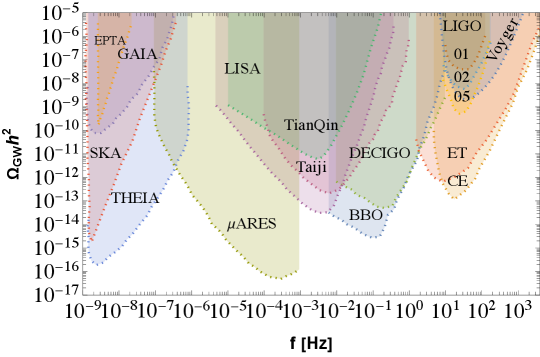
The main international collaborations working on the detection of GW using PTAs are the European Pulsar Timing Array (EPTA) Antoniadis et al. (2023a), the North American Nanohertz Observatory for Gravitational Waves (NANOGrav) Agazie et al. (2023b), the Indian Pulsar Timing Array (InPTA) Tarafdar et al. (2022) and the Parkes Pulsar Timing Array (PPTA) Zic et al. (2023). All these collaborations work together as the International Pulsar Timing Array (IPTA). The EPTA uses five 100 m class telescopes across Europe and monitors 41 pulsars at several frequencies. Using these five telescopes as a single telescope gives the highest overall sampling rate of pulsars among the existing PTAs. NANOGrav is a combined effort of US and Canada which uses single-dish telescopes that are among the world’s largest single-dish telescopes. NANOGrav currently monitors 49 pulsars. InPTA is an Indo-Japanese collaboration that makes use of the unique capabilities of the upgraded Giant Meterwave Radio Telescope (uGMRT) for monitoring a sample of nearby millisecond pulsars. PPTA uses the Parkes Observatory in Australia and can access pulsars in the Southern Hemisphere. It currently monitors 25 pulsars. Finally, the square kilometer array (SKA) Weltman et al. (2020) is an international radio telescope project that is being built in Australia (low-frequency) and South Africa (mid-frequency). It is expected to begin in 2028–29. Once ready, the SKA telescopes will be, by far, the most powerful instrument in the field of radio astronomy. Sensitivities for current and projected experiments we show in Fig. 1

II.1.2 Astrometry

The behaviour of light passing through a tensor perturbation is different to light passing through a scalar metric perturbation. The tensor perturbation is moving and the waves are transverse. The correct proceedure to recover the behaviour of light through a stochastic gravitational wave background is to make use of a geodesic equation. When one does so, as we will briefly show, one does not find that light undergoes a random walk such that the deviation grows with distance. Instead, the deviation is approximately independent of distance and depends only upon the strain sensitivity Kaiser and Jaffe (1997)

This remarkable fact allows us to search for correlated shifts in the angular velocity of many stars in order to reconstruct a gravitational wave background. The sensitivity of this approach grows linearly with time rather than the usual $1/\sqrt{T}$ convergence as the precision in measuring angular velocity kicks grows with time.

In this section, we will briefly explain these two facts before mentioning the reach of current and future astrometry experiments. For a more in-depth look, the reader is directed to refs. Kaiser and Jaffe (1997); Çalışkan et al. (2023); Moore et al. (2017); Klioner (2018); Wang et al. (2021, 2022). Let us begin with demonstrating the independence of the kicks with the distance from Earth. We begin with the geodesic equation in a gravitational wave background,

\ddot{d}(z)=\dot{H}(z)

(31)

where under the assumption of isotropy, we have

H(z)\sim\int k^{2}dkh_{a}(k)T_{a}(k)e^{i(1-\mu)kz}+c.c.

(32)

and

T_{+}=-\frac{1}{2}(1-\mu)\sqrt{1-\mu^{2})}(\cos\phi,\sin\phi),\ T_{x}=-\frac{1}{2}\sqrt{1-\mu^{2}}(\sin\phi,\cos\phi)\ .

(33)

We can then write a power spectrum of velocity kicks stars will have due to the gravitational wave background, as perceived by an observer on Earth,

$\displaystyle P_{\dot{d}}(k)$	$\displaystyle\sim$	$\displaystyle\langle H(0)\cdot H(z)\rangle$	(34)
	$\displaystyle\sim$	$\displaystyle\int dze^{ikz}\int q^{2}dqP(q)(T_{+}^{2}+T_{x}^{2})e^{i(1-\mu)kz}$	(35)
	$\displaystyle\sim$	$\displaystyle k\int dpP(p)(1-\cdots)\ ,$	(36)

where we have expanded to leading order in $k$ in order to eventually obtain the $k$ dependence of the power spectrum. In the above, $P(p)$ is the power spectrum for tensor perturbations

\displaystyle\langle h_{a}(k)h_{b}^{\ast}(p)\rangle=(2\pi)^{3}\delta(k-p)\delta_{ab}P(k).

(37)

The power spectrum of displacements will be related to the spectrum for kicks by $P_{d}\sim P_{\dot{d}}/k^{2}$ and we get the scaling

P_{d}\sim\frac{1}{k}\frac{\langle h^{2}\rangle}{k_{h}^{2}}\ .

(38)

The mean squared deviation averaged over a distance $D$ scales as

\displaystyle\langle d^{2}\rangle\sim\left.(kP_{d})\right|_{k=1/D}\sim D^{0}\ .

(39)

In other words, the size of the kick is independent of the distance between the source and the observer. We should therefore see a kick of the same size from a stochastic gravitational wave background which grows with the size of the strain. Looking at a large number of stars and searching for such correlated kicks therefore becomes an efficient method for finding a SGWB.

As for the impressive scaling of astrometry, to reconstruct the background, we need to track $N$ sources, for a time $T$ , resolving angles with a precision of $\Delta\Theta$ and therefore the angular velocity to a precision $\Delta\Theta/(T\sqrt{N})$ Book and Flanagan (2011). Our precision with the gravitational wave background then scales (remembering that $\Omega\sim h^{2}$ )

\Omega_{\rm GW}\lesssim\frac{\Delta\Theta^{2}}{NT^{2}H_{0}^{2}}\ .

(40)

Thus we see the powerful potential of using astrometry for gravitational wave detection - the sensitivity to a background scales much more efficiently with the lifetime of the experiment than other detectors.

Launched in 2013 by the European Space Agency, Gaia is a global space astrometry mission that maps more than a billion objects in the Milky Way. Detectors like Gaia Brown et al. (2018) use astrometric measurement to look for the low-frequency gravitational wave background Book and Flanagan (2011); Moore et al. (2017); Mihaylov et al. (2018, 2020); Garcia-Bellido et al. (2021). Recently, it was also shown that Gaia can be an important tool for probing GW with frequencies in range $\sim[10^{-9}-10^{-7}]$ Hz where the upper-frequency cut is set by the cadence and the lower frequency by the inverse lifetime of the experiment Moore et al. (2017); Mihaylov et al. (2018, 2020); Garcia-Bellido et al. (2021). Gaia is expected to observe a billion stars at an angular velocity resolution of about $100\mu$ as resulting in a strain sensitivity of

h_{\rm GW}\sim 10^{-14}\left(\frac{5{\rm years}}{T_{M}}\right)\ ,

(41)

with $T_{M}$ the mission lifetime. This makes it currently competitive with pulsar timing array measurements. There is a proposed upgrade to Gaia called Theia Boehm et al. (2017) which is expected to observe significantly more stars at a much higher angular resolution, which results in a strain sensitivity of

h_{\rm GW}\sim 10^{-14}\left(\frac{5{\rm years}}{T_{M}}\right)\left(\frac{\Delta\Theta_{\rm Theia}}{\Delta\Theta_{\rm Gaia}}\right)\sqrt{\left(\frac{N_{\rm stars,\ Gaia}}{N_{\rm stars,\ Theia}}\right)}\ ,

(42)

where $(\Delta\Theta_{x},N_{x})$ are the angular resolution and number of stars observed in experiment x. Exactly how much Theia will improve from Gaia is not yet clear, and recent estimates range from a factor of $100-600$ improvement in the strain sensitivity Garcia-Bellido et al. (2021); Çalışkan et al. (2023). A more exotic proposal aims to look for correlated kicks in asteroids in asteroid belt Fedderke et al. (2022) which is projected to achieve an impressive strain sensitivity of $10^{-19}$ at frequencies of $10\mu$ Hz. The sensitivity of Gaia as well as an approximate projection for Theia is given in Fig. 1.

We end this section by briefly mentioning another exotic idea to indirectly measure a stochastic gravitational wave background indirectly by observing their effect on astrophysical objects. Absent perturbations, binary systems follow elliptical orbits obeying Kepler’s laws. A stochastic gravitational wave background can perturb the system, giving and searches for deviations in the orbits of binary systems can be a window into gravitational wave backgrounds at the $\mu$ Hz range Blas and Jenkins (2022a, b).

II.1.3 Interferometers

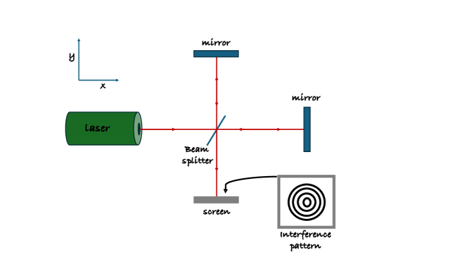
In 1887, Michelson-Morley for the first time used an interferometer to demonstrate the non-existence of ether in the Universe Michelson (1881). As interferometers are very sensitive to even tiny changes in a path difference, they are very useful in measuring small fluctuations in spacetime. In Fig. 2, we show a simple schematic of a Michelson-type interferometer.

In order to understand how the presence of GW affects the propagation of light in the interferometer Ricci and Brillet (1997); Aufmuth and Danzmann (2005); Maggiore et al. (2020), we first start with an assumption that GW has only a plus polarization and it arrives from the $z$ direction, so we have,

h_{+}(t)=h_{0}\cos\omega_{\rm GW}t.

(43)

Since the photons travel along a null geodesic $i.e.~{}ds=0$ this allows us to solve the change in the path length along a single direction in TT frame ⁴⁴4A similar calculation can also be performed in the proper frame. The computation of higher-order corrections becomes much more involved in the proper frame of the detector and hence for simplicity, we stick to the TT frame.

dx=\pm cdt(1-\frac{1}{2}h_{+}(t))

(44)

reflection and transmissions at the beam splitter give an overall phase shift of a $1/2$ . Let us consider a Michelson interferometer with arm length L where the beam splitter is at the origin at time $t_{0}$ with a phase $e^{-i\omega_{L}t_{0}}$ . The phase shift from the gravitational wave due to the field going through the x and y arms are

\Delta\phi_{x}=-\Delta\phi_{y}=h_{0}\frac{\omega_{L}L}{c}{\rm sinc}(\omega_{\rm GW}L/c)\cos[\omega_{\rm GW}(t-L/c)]\ .

(45)

The total power at the detector is related to a phase, $\phi_{0}$ , set by the experimenter

P=\frac{P_{0}}{2}\left\{1-\cos[2\phi_{0}+\Delta\phi_{\rm Mich}(t)]\right\}\ .

(46)

For a given signal that peaks at a a frequency $f_{p}=\omega_{\rm GW}/2\pi$ , the boost in power is maximal when

L=750{\rm km}\left(\frac{100{\rm Hz}}{f_{p}}\right)

(47)

Ground-based detectors don’t achieve an arm length 100s of kilometers long, Ligo and Virgo has arms of 4 and 3km respectively Aasi et al. (2015); Abbott et al. (2016a); Buikema et al. (2020); Tse et al. (2019); Acernese et al. (2015, 2019). However, to achieve a larger effective path length they use a Fabry-Perot cavity Aasi et al. (2015); Abbott et al. (2016a). Such a cavity traps light within it for a long time. If a Fabry-Perot cavity is a few kilometers long and has light trapped within it for around 100 trips between the edges of the cavity, then the gravitational wave detector can be sensitive to frequencies as low as $1-100$ Hz. The phase shift in the Fabry-Perot cavity in the presence of the GW along the $x$ and $y$ axis is given by

\Delta\phi_{x}=-\Delta\phi_{y}\simeq h_{0}2\frac{\omega_{L}L}{c}\frac{\mathcal{F}}{\pi}\frac{1}{[1+(4\pi f_{p}\tau_{s})^{2}]^{1/2}},

(48)

where $\mathcal{F}$ is known as the finesse of the cavity which is defined as the ratio of free spectral range ( $\Delta\omega_{L}$ ) to the full-width half maximum and $\tau_{s}$ is the storage time of the cavity, $i.e.$ the average time spent by a photon in the cavity.

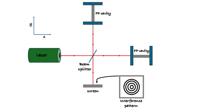
Comparing Eq. (48) with Eq. (45) we find that in a Fabry-Perot, the sensitivity of a phase shift is enhanced by a factor of $(2/\pi)\mathcal{F}$ in comparison to what is obtained in a Michelson interferometer.

These interferometers are also subjected to various types of noises that can affect the detection of GW signals, for example, optical read-out noises which are a combination of the shot noises of a laser (that results from the discretization of photons) and radiation pressure (generated from pressure exerted by the laser beam on the mirrors), displacement noises which are generated by the movement of a test mass and are not induced by the GWs. Other noises that can influence the detection of GW signals are Seismic and Newtonian noise that results from local movements like traffic, trains, or surface waves that shake the suspension mechanism of the interferometer, thermal noises that are induced by the vibrations in mirrors and suspensions or the fluctuations in the test masses, etc. Apart from these sources, there exist several other sources of noise that can affect the detection of GW by an interferometer. Irrespective of the kind of noises, all of them can be characterized using their NSR which is further used to calculate the signal-to-noise ratios. For a detailed discussion, we refer the readers to Maggiore (2007).

With the first observation of the GW signals in 2015 by LIGO collaborations, the role and significance of interferometers in GW detection have increased manyfold. At present, there exist several earth-based interferometers that are currently running and are aiming to detect more signals. Among them, the most popular ones are at Hanford and Livington both located in the US with 4 km arms which are run by LIGO collaborations Aasi et al. (2015); Abbott et al. (2016a); Buikema et al. (2020); Tse et al. (2019), and the VIRGO interferometer Acernese et al. (2015, 2019) with arms of 3 km located near Pisa, Italy. KAGRA Akutsu et al. (2019); Aso et al. (2013) is another recently built underground laser interferometer with 3 km arm lengths located in Japan. Other smaller detectors like GEO600 (arms with 600 m) and TAMA (arms with 600 m) are situated in Hannover, Germany, and Tokyo, Japan respectively. Due to the longer arm lengths, better sensitivity can be achieved by detectors like LIGO, VIRGO, and KAGRA.

Apart from these existing detectors, there have been proposals to build next-generation detectors with better sensitivity. Cosmic Explorer Reitze et al. (2019) is one of them which features two L-shaped detectors one with arm lengths of 40 km and another with 20 km arm lengths. The Einstein Telescope Maggiore et al. (2020) is another proposed underground interferometer with arms of 10 km in length and it is expected to start its observations in 2035. Other than these ground-based detectors, there are several proposals for space-based detectors like LISA (Laser Interferometer Space Antenna) Amaro-Seoane et al. (2017), $\mu-$ ARES Sesana et al. (2021), TianQin Luo et al. (2016), Taiji Hu and Wu (2017), Voyger Adhikari et al. (2020), DECIGO ( DECi-hertz Interferometer Gravitational wave Observatory) Kawamura (2019). These space-based interferometers have a few advantages over ground-based detectors. For starters, larger arm lengths can be achieved in space which in turn can help in increasing the sensitivity, and various noises that provide a hindrance for the earth-based detectors can easily be avoided. Space-based detectors are the future of GW detection as they will help us further in unfolding the mysteries of the early Universe. For the sensitivity of a selection of these detectors see Fig. 1

II.2 Cosmological detectors

In the era of precision cosmology, state-of-the-art analysis of the cosmic microwave background (CMB) and the abundance of light elements shed light on the gravitational wave background. First, both the production of light elements and the CMB are highly sensitive to the expansion rate of the Universe during each epoch (around 1 second and 1 million years respectively). If there is a gravitational wave background, the total radiation density is slightly higher than it would be otherwise. Precision fits to data for both the CMB and the abundances of light elements put a limit on the extra radiation allowed that is usually written in terms of the effective number of extra relativistic freedom,

N_{\rm eff}\leq\left\{\begin{array}[]{cc}2.88\pm 0.54&\text{ BBN~{}\cite[cite]{\@@bibref{Authors Phrase1YearPhrase2}{Pitrou:2018cgg}{\@@citephrase{(}}{\@@citephrase{)}}}}\\ 3.00\pm 0.34&\text{ CMB ~{}(lensing+BAO) ~{}\cite[cite]{\@@bibref{Authors Phrase1YearPhrase2}{Planck:2018vyg}{\@@citephrase{(}}{\@@citephrase{)}}}}\\ 3.01\pm 0.15&\text{ (BBN+CMB) ~{}\cite[cite]{\@@bibref{Authors Phrase1YearPhrase2}{Pitrou:2018cgg}{\@@citephrase{(}}{\@@citephrase{)}}}}\end{array}\right.

(49)

To make use of this bound, we need to convert the additional gravitational wave radiation from its stochastic background into an effective amount of relativistic degrees of freedom. After electron-positron annihilation at 0.5 MeV, the ratio of gravitational radiation to electromagnetic radiation becomes constant. This means for both BBN and CMB observables we can, to a good approximation, use

\Delta N_{\rm eff}=\frac{8}{7}\left(\frac{11}{4}\right)^{\frac{4}{3}}\frac{\Omega_{\rm GW}^{0}}{\Omega_{\gamma}^{0}}

(50)

where the 0’s indicate the values of their abundances today. The total gravitational radiation is of course

\displaystyle\Omega^{0}_{\rm GW}=\int\frac{df}{f}\Omega_{\rm GW}^{0}(f)\ .

(51)

The second cosmological observable is temperature-polarization B-modes in the CMB, which are induced by gravitational waves (for a review see Kamionkowski and Kovetz (2016)). The CMB is sensitive to very low frequencies, around $10^{-17}$ Hz Lasky et al. (2016). The only known candidate to produce a source at such frequencies is inflation itself. We will cover higher frequency signals from gravitational waves due to a blue tilted spectrum in section VI

II.3 High frequency proposals

Many cosmological gravitational wave sources are strongly peaked at a frequency that approximately corresponds to the Hubble scale at the time the source was produced. We will get into specifics in later sections. For now, we wish to draw attention to the fact that the higher the frequency, the higher the energy scale a gravitational wave detector can probe. The maximum temperature the Universe can reach is at around the GUT scale, depending upon the details of preheating.⁵⁵5It depends upon the details of the model. If there is an instability scale, then finite temperature corrections can render the Universe unstable Delle Rose et al. (2016), alternatively, gravitational freezeout could clash with $\Delta N_{\rm eff}$ bounds for a modestly higher temperature Ringwald et al. (2021) This means that gravitational wave cosmology has an incredible scope to probe physics at scales we could only dream of on Earth. On the other hand, the challenge is enormous.

As mentioned in the previous subsection, gravitational waves act as a source of dark radiation in the early Universe, mildly changing the expansion rate during Big Bang nucleosynthesis and recombination. The degree to which this expansion rate can change is restricted by observation. To shed light on any cosmological events before Big Bang nucleosynthesis, a gravitational wave detector must be more sensitive than limits on extra dark radiation. Since the abundance of gravitational radiation is related to the strain by $\Omega_{\rm GW}\sim h^{2}f^{2}$ , the target strain sensitivity needed to beat limits on dark radiation grows quadratically with the frequency. As such, no proposal currently exists that can uncontroversially probe gravitational waves at higher than around 1 kHz and beat the bounds on dark radiation. Even still, the opportunities presented by high-frequency gravitational wave physics have led to some ingenious proposals which are summarized in a living review in ref. Aggarwal et al. (2021). As yet, unfortunately there are no concrete proposal that can beat the bounds from $\Delta N_{\rm eff}$ on high frequency gravitational waves, so we do not cover any proposal in detail here. However, this is an active field to keep an eye on and we refer the reader to the above mentioned review for the current state of affairs.

III Gravitational waves from cosmic phase transitions

Gravitational waves from first-order cosmic phase transitions is a scenario that has been the focus of intense attention for the last decade Mazumdar and White (2019). The concepts involved are in some ways quite familiar, everyone encounters phase transitions in their daily lives, most notably when water boils or freezes. A phase transition can occur when the ground state of a system is dependent on the temperature. In the case of boiling water, the high temperature phase is vapour which nucleates in a medium of the low temperature phase which is liquid. As the expanding Universe describes a system that is cooling, we will instead be considering cases where the Universe boils as it cools, and the bubbles contain the low temperature phase. As familiar as the concepts are, theoretically handling such an out-of-equilibrium quantum field theory has challenged the field for decades. In this section, we first make use of classical phase transitions to build an intuition for the subject before outlining the narrative of a cosmic phase transition, and the range of motivations for considering them and we review our current best understanding of how to model them.

III.1 Nucleation of bubbles

It is instructive to start with classical nucleation theory. Consider a bubble of a low-temperature phase nucleating in the background of the high-temperature phase. The Energy of the bubble of radius $R$ can be expressed in terms of a pressure term, $\Delta p$ , that prompts expansion and a surface tension term, $\sigma$ , that attempts to collapse the bubble Abraham (1974)

E=-\frac{4\pi}{3}R^{3}\Delta p+\sigma 4\pi R^{2}\ .

(52)

Such a bubble has a maximum in energy when the radius is at a critical value where the pressure and surface tension cancel each other out at $R=2\sigma/\Delta p$ . Above this critical radius, the pressure begins to overwhelm the surface tension and the bubble expands. The nucleation rate is the exponential of the energy of a bubble with a critical radius divided by the temperature

\Gamma\sim e^{-\frac{16\pi\sigma^{3}}{3\Delta p^{2}T}}

(53)

so we see that a large surface tension suppresses nucleation and is the main proxy for the strength of a transition. The pressure difference between the two phases will grow as the system cools, so the nucleation rate will increase at least as long as $\Delta p$ grows faster than the square root of temperature. In practice, $\Delta p$ can reach a maximum and it is possible for a phase transition to never complete.

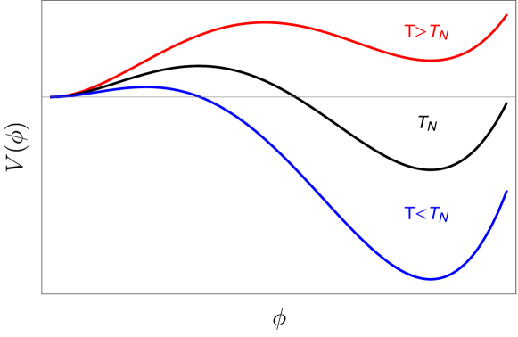
A cosmic phase transition has three additional ingredients to classical nucleation theory - a field-theoretic treatment, an expanding background, and quantum corrections. Let us begin by considering how field theory modifies the classical nucleation prescription. It is most common to consider phase transitions driven by the thermal evolution of the effective potential, sketched in Fig. 4, for a scalar field which we will denote as $\phi$ . In such a case, we can derive the existence and behaviour of a bubble as a classical solution to the equations of motion. We simplify our lives by considering only spherical bubbles, Wick rotating and assuming the thermal field theory is periodic in time with a period $1/T$ . This allows us to make the approximation $\int dt\to\frac{1}{T}$ , in which case the equations of motion are

\frac{\partial^{2}\phi}{\partial r^{2}}+\frac{2}{r}\frac{\partial\phi}{\partial r}=\frac{\partial V}{\partial\phi}.

(54)

A solution to this is of course that the field occupies an extremum where the gradient of the potential vanishes. However, imagine the above equation with the $r$ coordinate replaced with time - it now describes the equations of motion of a ball on a hill of shape $-V$ with a strange time-dependent friction term. If we place the ball close to its maximum value, it will roll down towards the other local maximum. An initial condition that is too high will result in the ball rolling past the local maximum and continuing forever. If the initial condition is too low, the ball will roll around forever in the minimum connecting the two maxima. However, there is a Goldilocks solution where the ball starts in just the right place to land on the top of the local maximum.

Returning our imagination to the field theory case with radial rather than time derivatives, the solution we have found is of a spherically symmetric object that is in the true vacuum at the center and becomes more like the false vacuum as we venture further out in radius. Or, in other words, it is a bubble of true vacuum nucleating in the medium of false vacuum Coleman (1977).

So let us connect with what we learnt in nucleation theory. First, we can estimate the nucleation probability with the path integral formalism. We can take a saddle point approximation to then estimate the path integral as the exponential of the action Coleman (1977); Callan Jr and Coleman (1977); Linde (1981) ⁶⁶6It is interesting to point out that a phase transition may also proceed via bubbles seeded by impurities. This idea has been recently discussed in Blasi and Mariotti (2022); Agrawal et al. (2023) the context of the electroweak phase transition and and the corresponding implications for gravitational waves from sound waves have been investigated in Blasi et al. (2023a),

\Gamma\sim e^{-S}\sim e^{-S_{E}/T}

(55)

where in the second line we have again used the approximation that $\int_{0}^{\beta}dt\to\beta$ , leaving a Euclidean action that involves only a spatial integral. If we approximate the bubble profile as having a very thin wall, it is possible to make a direct analogue of classical nucleation theory,

S_{E}(\phi_{\rm bubble})=\frac{16\pi\sigma^{3}}{\Delta p^{2}}

(56)

where $\Delta p=\Delta V$ and the surface tension can be calculated by integrating the potential from the false vacuum $v_{1}$ to the true one $v_{2}$ ,

\sigma={\rm Re}[\int_{v_{1}}^{v_{2}}d\phi\sqrt{2V}]\ .

(57)

The thin wall approximation is only accurate very close to the critical temperature, however, we can nonetheless learn physical insight from the above. Recall that the strength of the transition is controlled by the surface tension. The surface tension grows with the height and width of the barrier separating the two phases. In the case of a scalar field theory, the surface tension will grow with the number of bosonic degrees of freedom that are made heavy by the change in phase as the change in mass of such Bosons. It is also possible in scalar field theories for there to be a large contribution to the surface tension from the tree-level shape of the potential if cubic terms are permitted by the symmetries of a theory. Specifically, one can have a field direction, $\phi$ , where the tree level potential has the form $a\phi^{2}+b\phi^{3}+c\phi^{4}$ and there is a tree level barrier between the minima. We thus expect these two paths to be the main avenues for producing a strong first-order phase transition - a large number of bosonic degrees of freedom gaining a large mass in the new phase and the symmetries of the theory allowing the potential to have a tree-level barrier.

Confining transitions are much more difficult to theoretically model than transitions involving the vacuum expectation value of a scalar field. However, the methods we do have seem to find similar wisdom where large changes in mass Croon et al. (2019b) of large degrees of freedom can lead to stronger transitions Lucini et al. (2005); Datta and Gupta (2010); Croon et al. (2019b); Garcia-Bellido et al. (2021).

The last pieces of the picture needed to mimic the situation of the early Universe are the quantum effects and the expanding background. A modest quantum effect arises from the fluctuations around the bubble solution to the classical equations of motion. This results in a logarithmic correction to the effective action, and therefore a modification of the prefactor. A more dramatic effect is in the evolution of the effective potential - all thermal corrections are due to loops.⁷⁷7We acknowledge that the precise demarcation between what is truly quantum and what isn’t can be subtle. For this review, we use the term quantum to refer to things that would vanish if $\hbar\to 0$ which, perhaps counterintuitively, is the case for all finite temperature corrections to a quantum field as all finite temperature terms are loop-induced The fact that these loop corrections need to be large enough to qualitatively change the features of the tree level effective potential signals that we should worry about the efficacy of perturbation theory! This issue we will return to shortly. Finally, the expansion of the Universe means that the phase transition does not begin the moment it becomes energetically favourable for there to be a change in the ground state. Instead, we should compare the nucleation rate to the expansion of the Universe. When the nucleation rate is large enough that there is at least one critical size bubble per Hubble volume per Hubble time, the phase transition can be thought to begin. However, if the nucleation rate does not further increase from this minimum rate, the phase transition could never be complete as the bubbles cannot catch up to the expanding volume around them. Because of this, the time scale of the phase transition, $\beta^{-1}$ ⁸⁸8Unfortunately it is a confusing convention to have both the inverse time scale and the inverse temperature denoted by $\beta$ . We will follow this convention in this review. is controlled not by the nucleation rate, but its first (and occasionally second Athron et al. (2023b, c)) derivative,

\beta\sim\frac{1}{\Gamma}\frac{d\Gamma}{dt}\to\frac{\beta}{H}\sim T\frac{d(S_{E}/T)}{dT}\ .

(58)

III.2 Effective potential and action at finite temperature

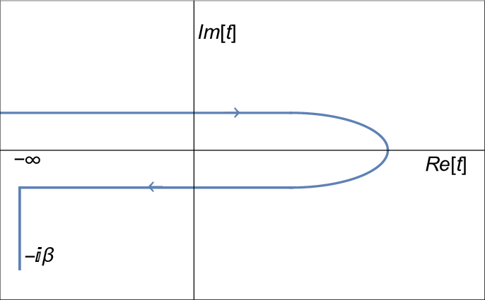
There are in general two ways people tend to include temperature corrections to quantum field theory - the imaginary time formalism and the real time or closed time path formalism. The closed time path formalism assumes that the system was at once in equilibrium in the past. Starting with the finite temperature density matrix, one can then derive using the interaction picture of quantum mechanics that the expectation value of an operator is evaluated using the time contour shown in Fig. 5. A consequence of this unusual time contour is that there are no longer just time-ordered and time-anti-ordered propagators, there are also mixed two-point correlators that involve on field moving in opposite directions in time. The propagators in equilibrium are just a zero temperature contribution (which vanishes in the case of the mixed correlators) summed with a finite temperature piece. This means that when one writes the corrections to the effective potential by calculating the 1-particle-irreducible loop diagrams, the result is a sum of the loop corrections at zero temperature and the finite temperature corrections. The closed time path formalism has the potential to handle departures from equilibrium, though this review is not aware of any attempt to take advantage of this in gravitational wave calculations.

In equilibrium, an alternative formalism considers the propagators in imaginary time and in equilibrium. In this case, after Wick rotating, the thermal field theory becomes periodic in time. As a result, the $k_{0}$ modes become discrete, and are known as Matsubara modes and the $dk_{0}$ integrals are replaced by a sum over these modes. The result is not obviously equivalent to the sum of zero and finite temperature pieces that one derives in the closed time path formalism. However, as long as one approximates the background plasma as being in equilibrium⁹⁹9calculating the effective potential in a non-equilibrium background was recently done at zero temperature Garbrecht and Millington (2017), though we are not aware of an attempt to do the equivalent at finite temperature, then after some massaging, the result of both approaches are the same

V_{T}=\sum_{i\in{\rm bosons}}n_{i}\frac{T^{4}}{2\pi^{2}}J_{B}\left(\frac{m_{i}^{2}}{T^{2}}\right)-\sum_{i\in{\rm fermions}}n_{i}\frac{T^{4}}{2\pi^{2}}J_{F}\left(\frac{m_{i}^{2}}{T^{2}}\right)\ ,

(59)

where the thermal functions have the form

	$\displaystyle J_{B}(\bar{z}^{2})$	$\displaystyle=$	$\displaystyle\int_{0}^{\infty}dxx^{2}\log\left[1+e^{-\sqrt{x^{2}+\bar{z}^{2}}}\right]\sim\frac{\bar{z}^{2}}{24}-\frac{\bar{z}^{3}}{12\pi}+\cdots$		(60)
	$\displaystyle J_{F}$	$\displaystyle=$	$\displaystyle\int_{0}^{\infty}dxx^{2}\log\left[1-e^{-\sqrt{x^{2}+\bar{z}^{2}}}\right]\sim-\frac{\bar{z}^{2}}{48}\ .$		(61)

In the above, the right-hand approximations are the high-temperature expansions when $\bar{z}=m/T$ is small.

We can now sketch how a first-order phase transition is generated. Consider a Bosonic field whose mass scales as $m_{g}=g\phi$ where $\phi$ is the scalar field undergoing a change in its vacuum expectation value during the phase transition. In such a case, the thermal corrections to the potential due to this field in the high-temperature limit is

\Delta V_{T}=\frac{g^{2}\phi^{2}T^{2}}{24}-\frac{g^{3}\phi^{3}T}{12\pi}+\cdots

(62)

The second term in the above equation produces a barrier as the full potential can have three consecutive terms with alternating signs. Let the tree-level potential be of the form

V=\mu^{2}\phi^{2}+\lambda\phi^{4}\ .

(63)

After rescaling $V\to\Lambda^{4}\tilde{V}$ and $\phi\to v\varphi$ where $v$ is the vacuum expectation value, then absorbing a redundant parameter into the definition of $\Lambda$ , one can rewrite the potential and mass as¹⁰¹⁰10The specific redefinitions are $\mu^{2}=\frac{1}{2v^{2}}\Lambda^{4}$ and $\lambda=\frac{\Lambda^{4}}{4v^{4}}$

$\displaystyle\tilde{V}$	$\displaystyle=$	$\displaystyle\Lambda^{4}\left(-\frac{1}{2}\left[\frac{\varphi}{v}\right]^{2}+\frac{1}{4}\left[\frac{\varphi}{v}\right]^{4}\right)$	(64)
$\displaystyle m_{\phi}$	$\displaystyle=$	$\displaystyle\sqrt{2}\frac{\Lambda^{2}}{v}$	(65)
$\displaystyle m_{g}$	$\displaystyle=$	$\displaystyle gv\ ,$	(66)

where $m_{\phi}$ is the mass of the field $\phi$ . If we consider the temperature at which the potential is double-welled, that is the critical temperature, the surface tension scales as

\sigma\approx\frac{gm_{g}^{5}}{m_{\phi}^{2}}

(67)

as long as $3\pi^{2}m_{\phi}^{2}>>g^{2}m_{g}^{2}$ . This limit is chosen to simplify our expression but is similar to the regime at which the high-temperature regime is valid. Regardless, we are only interested in a qualitative picture and indeed we see from the above that the strength of the phase transition grows with the ratio of the mass of the masses as we expected from our discussion in the previous section. Repeating the above for $n$ copies of $m_{g}$ finds that the strength of the transition grows with $n$ . So we find a rule of thumb - the strength of the transition grows with the number of bosonic degrees of freedom becoming nonrelativistic during the transition and the ratio of their masses to the mass of the dynamical scalar. Remarkably this seems to be true of chiral transitions as well Croon et al. (2019b). From this rule of thumb, we can see why the Standard model is expected to have a crossover transition. The Higgs boson is in fact heavier than all gauge bosons that acquire a mass during electroweak symmetry breaking and the size of the gauge group, $SU(2)\times U(1)$ , doesn’t have enough gauge bosons to compensate for such a small ratio.¹¹¹¹11Strictly speaking, there is no surface tension for a crossover transition. However, analysing the surface tension does give the correct wisdom about how to make the transition stronger

III.3 Possible sources

If the reheating temperature reached at least the electroweak scale, then it is likely that our Universe experienced at least two changes in its ground state - an epoch of electroweak symmetry breaking at temperatures of around 100 GeV and an epoch where the quark-gluon plasma hadronizes at around 100 MeV. As mentioned above, both transitions are crossovers in the Standard Model at the low densities expected in the early Universe Kajantie et al. (1996c, b, 1997); Csikor et al. (1999); D’Onofrio and Rummukainen (2016); Aoki et al. (2006); Bhattacharya et al. (2014). However, this picture can change if the physics beyond the Standard Model permits it, and these transitions could occur via the nucleation and percolation of bubbles of the low-temperature phase. Such a spectacular process of the early Universe boiling for an epoch naturally leads to a gravitational wave signal that could be visible today.

In the case of electroweak symmetry breaking, the most common ways to modify it to catalyze a strong first-order phase transition are

1

Introduce more bosonic degrees of freedom that couple to the Higgs. The canonical examples are the two Higgs doublet model Dorsch et al. (2013); Basler et al. (2017); Dorsch et al. (2016, 2017a); Bernon et al. (2018); Dorsch et al. (2017b); Andersen et al. (2018); Kainulainen et al. (2019); Wang et al. (2020b); Su et al. (2021); Davoudiasl et al. (2021); Biekötter et al. (2021); Zhang et al. (2021); Aoki et al. (2022); Gonçalves et al. (2022); Phong et al. (2023); Biekötter et al. (2023a); Anisha et al. (2022); Atkinson et al. (2022); Biekötter et al. (2023b); Gonçalves et al. (2023); Gráf et al. (2022); Arcadi et al. (2023) (including the inert doublet model Blinov et al. (2015b); Huang and Yu (2018, 2018); Paul et al. (2019, 2019); Fabian et al. (2021); Benincasa et al. (2022); Paul et al. (2022); Jiang et al. (2023); Astros et al. (2023); Benincasa et al. (2023)) and the light stop mechanism Carena et al. (1996); Espinosa (1996); Delepine et al. (1996); Cline and Kainulainen (1996); Losada (1997); Laine (1996); Bodeker et al. (1997); de Carlos and Espinosa (1997); Cline and Moore (1998); Losada (1999); Laine and Rummukainen (2001); Carena et al. (2009); Delgado et al. (2012); Carena et al. (2013); Chung et al. (2013); Huang et al. (2013); Laine et al. (2013); Liebler et al. (2016). However, it is also possible with a scalar electroweak triplet Patel and Ramsey-Musolf (2013); Huang and Yu (2018); Chala et al. (2019); Baum et al. (2021); Kazemi and Abdussalam (2021); Baldes et al. (2021a); Azatov et al. (2021), and complex Jiang et al. (2016); Chiang et al. (2018); Ahriche et al. (2019); Kannike et al. (2020); Chen et al. (2020b); Cho et al. (2021); Schicho et al. (2022); Di Bari and Rahat (2023), a real scalar singlet(s) Espinosa and Quiros (1993); Profumo et al. (2007); Cline et al. (2009); Cline and Kainulainen (2013); Cline et al. (2013); Katz and Perelstein (2014); Profumo et al. (2015); Vaskonen (2016); Hashino et al. (2016); Chao et al. (2017); Matsui (2018a); Kang et al. (2018); Alves et al. (2019); Shajiee and Tofighi (2019); Beniwal et al. (2019); Matsui (2018b); Kannike et al. (2020); Demidov et al. (2022); Cline et al. (2021); Cao et al. (2022); Athron et al. (2023a); Alanne et al. (2020) or a composite Higgs model Bian et al. (2019); Xie et al. (2020).
2

Introduce an effective tree-level barrier between the true and false vacuum. This means that the surface tension between the two phases may not vanish even at zero temperature. The two most common ways of achieving this are through an effective cubic coupling from a gauge singlet, $sH^{\dagger}H$ , or having a heavy degree of freedom integrated out such that the effective potential of the Higgs has alternating signs of the form Grojean et al. (2005); Bodeker et al. (2005); Delaunay et al. (2008); Balazs et al. (2017); de Vries et al. (2018); De Vries et al. (2019); Chala et al. (2018); Ellis et al. (2019b)

$V=\mu^{2}H^{\dagger}H-\lambda(H^{\dagger}H)^{2}+\frac{1}{\Lambda^{2}}(H^{\dagger}H)^{3}\ .$ (68)

Unfortunately, the Standard Model requires such a dramatic change to its effective potential to catalyze a first-order transition, that there is only one UV complete model that can be accurately characterized by the above potential - the real scalar singlet extension of the Standard Model Postma and White (2021). This renders an effective field theory approach to be of questionable utility.

A more exotic approach is to have a multi-step transition Weinberg (1974); Land and Carlson (1992); Hammerschmitt et al. (1994); Patel and Ramsey-Musolf (2013); Patel et al. (2013); Blinov et al. (2015a); Inoue et al. (2016); Blinov et al. (2015a); Ramsey-Musolf et al. (2018); Croon and White (2018); Angelescu and Huang (2019); Niemi et al. (2019); Morais et al. (2020); Morais and Pasechnik (2020); Niemi et al. (2021); Cao et al. (2022) where the direction the field goes during the phase transition is no longer from the origin. Turning to the case of the QCD transition, it was first argued by Pisarski and Wilczeck that one needs a minimum number of light flavours in order for chiral symmetry breaking to be strongly first order Pisarski and Wilczek (1984), this has been demonstrated on the Lattice for $N_{F}\geq 3$ Iwasaki et al. (1996). All models of the QCD transition seem to suggest that at large baryon chemical potential, the QCD transition becomes strongly first order Costa et al. (2009); Marquez and Zamora (2017); Vovchenko et al. (2019); Chen et al. (2019); Câmara Pereira et al. (2020); Gao and Pawlowski (2020, 2021); Gao and Oldengott (2022); Gao et al. (2023). However, the lattice is yet to confirm the existence of a critical endpoint at which the baryon density is large enough to change the nature of the transition Bazavov et al. (2017); Ding (2021). Finally, the pure Yang Mills theory is easier to model due to the absence of fermions. We know that pure Yang Mills always yields a first-order phase transition. We therefore have three possible methods for inducing a strong QCD phase transition

1

Render the mass of the strange quark dynamical such that it is much lighter in the early Universe. This can be achieved through a flavon field which renders the effective coupling between the Higgs and strange quark to be proportional to the vacuum expectation value of the flavon field Davoudiasl (2019). Another option is to have Higgs field supercool until the QCD era, at which the QCD transition catalyzes both electroweak and chiral symmetry breaking Witten (1981); von Harling and Servant (2018); Wong and Xie (2023); Li et al. (2023d); Zhao et al. (2023a).
2

In principle one could use flavon fields to render all quarks heavy in the early Universe. In such a case one would have a strong first order glueball transition. This option has not been analyzed in the literature, though glueball transitions have Halverson et al. (2021); Bigazzi et al. (2020, 2021); Huang et al. (2021); Wang et al. (2020a); Kang et al. (2021); Garcia-Bellido et al. (2021); Morgante et al. (2023). We include it for completeness.
3

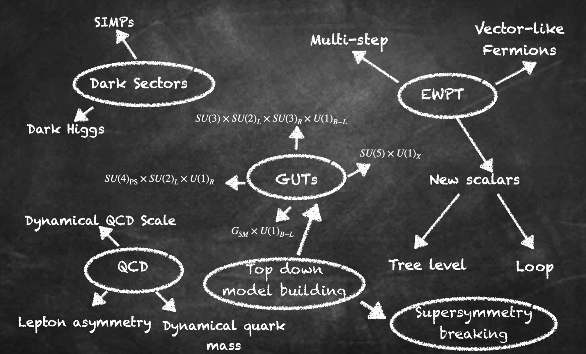
A third option is to have a large baryon chemical potential. The only known way to do this is to have a large lepton asymmetry Schwarz and Stuke (2009); Caprini et al. (2010); Middeldorf-Wygas et al. (2022).

While the QCD and electroweak eras are arguably the most well-motivated epochs to search for (as we know that at least a change in ground state likely occurred) there are many more motivations for a strong first-order phase transition in the early Universe. A popular model to realize a scale-invariant potential as described in section III.4.2 is B-L breaking Jinno and Takimoto (2017b); Chao et al. (2020); Brdar et al. (2019b); Okada and Seto (2018); Marzo et al. (2019); Bian et al. (2021); Hasegawa et al. (2019b); Ellis et al. (2019a); Okada et al. (2020) (or B/L breaking Fornal and Shams Es Haghi (2020); Bosch et al. (2023)). Additionally people have considered phase transitions in neutrino mass models Li et al. (2021); Di Bari et al. (2021); Zhou et al. (2022); Costa et al. (2022b), GUT symmetry breaking chains Hashino et al. (2018); Huang and Zhang (2019); Croon et al. (2019a); Brdar et al. (2019a); Huang et al. (2020b); Gráf et al. (2022); Fornal et al. (2023), flavour physics Greljo et al. (2020); Fornal (2021), supersymmetry breaking Fornal et al. (2021); Craig et al. (2020); Apreda et al. (2002); Bian et al. (2018), hidden or dark sectors Schwaller (2015); Baldes and Garcia-Cely (2019); Breitbach et al. (2019); Croon et al. (2018); Hall et al. (2020); Baldes (2017); Croon et al. (2020b); Hall et al. (2023, 2020); Chao et al. (2021); Dent et al. (2022); Helmboldt et al. (2019); Aoki and Kubo (2020); Helmboldt et al. (2019); Croon et al. (2020a, 2019b); Alanne et al. (2020); Garcia-Bellido et al. (2021); Huang et al. (2021); Halverson et al. (2021); Kang et al. (2021); Fornal and Pierre (2022); Costa et al. (2022a); Benincasa et al. (2023) and axions Dev et al. (2019); Von Harling et al. (2020); Delle Rose et al. (2020). The full landscape of ideas we show in Fig. 6.

Most of the above involve phase transitions involving scalar fields. However, it takes different technology to model a confining transition. The typical approach in the literature is to model some condensate as a scalar field and consider its effective potential Croon et al. (2019b); Helmboldt et al. (2019). In the case of the linear Sigma model, one writes an effective potential for the quark condensate where the parameters of the potential are free and the one-loop corrections are derived in exact analogue with a scalar field theory Croon et al. (2019b)

V(\Sigma)=-m_{\Sigma}^{2}{\rm Tr}\left(\Sigma\Sigma^{\dagger}\right)-(\mu_{\Sigma}{\rm det}\Sigma+h.c.)+\frac{\lambda}{2}\left[{\rm Tr}(\Sigma\Sigma^{\dagger})\right]^{2}+\frac{\kappa}{2}{\rm Tr}\left(\Sigma\Sigma^{\dagger}\Sigma\Sigma^{\dagger}\right)

(69)

where $\Sigma_{ij}\sim\langle\bar{\psi}_{Rj}\psi_{Li}\rangle$ is the quark condensate that is decomposed as

\Sigma_{ij}=\frac{\phi+i\eta^{\prime}}{\sqrt{2N_{F}}}\delta_{ij}+X^{a}T^{a}_{ij}+i\pi^{a}T_{ij}^{a}

(70)

and $\phi$ is what acquires a vacuum expectation value. The determinant term in the effective potential above arises from instanton effects. In this model, it seems that the strength of the gravitational wave signal grows with the number of light flavours (at least going from 3 flavours to 4) and the hierarchy between the meson and the axion mass.

For the Nambu-Jona-Lasino model (NJL), again an effective potential is written for mesons but the mesons are non-propagating and the loop corrections are derived from considering quarks running in the loop Nambu and Jona-Lasinio (1961a, b); Klevansky (1992); Holthausen et al. (2013)

$\displaystyle V_{0}^{\rm NJL}(\sigma)$	$\displaystyle=$	$\displaystyle\frac{3}{8G}\bar{\sigma^{2}}-\frac{G_{D}}{16G^{3}}\sigma^{3}$	(71)
$\displaystyle V_{\rm CW}^{\rm NJL}(\sigma)$	$\displaystyle=$	$\displaystyle-\frac{3n_{c}}{16\pi^{2}}\left[\Lambda^{4}\log\left(1+\frac{M^{2}}{\Lambda^{2}}\right)-M^{4}\log\left(1+\frac{\Lambda^{2}}{M^{2}}+\Lambda^{2}M^{2}\right)\right]$	(72)
$\displaystyle V_{\rm T}^{\rm NJL}(\sigma,T)$	$\displaystyle=$	$\displaystyle 6n_{c}\frac{T^{4}}{\pi^{2}}J_{F}(M^{2}/T^{2})$	(73)
$\displaystyle M$	$\displaystyle=$	$\displaystyle\bar{\sigma}-\frac{G_{D}}{8G^{2}}\bar{\sigma^{2}}$	(74)

where $G$ and $G_{D}$ are free parameters. Unlike the linear sigma model. The latter model can be enhanced by adding the Polyakov loop resulting in a gluon potential Fukushima and Skokov (2017). If the model in question has three colours, lattice data can be used to model the gluon contribution to the potential,

{\cal L}_{\rm PNJL}^{\rm MFA}={\cal L}_{\rm NJL}^{\rm MFA}-V_{\rm Glue}(L,T)

(75)

T^{-4}V_{\rm glue}(L,T)=-\frac{1}{2}a(T)L\bar{L}+b(T)\log\left[1-6L\bar{L}-3(L\bar{L})^{2}+4(L^{3}+\bar{L}^{3}\right]

(76)

	$\displaystyle a(T)$	$\displaystyle=$	$\displaystyle 3.51-2.47\frac{T_{\rm glue}}{T}+15.2\left(\frac{T_{\rm glue}}{T}\right)^{2}$		(77)
	$\displaystyle b(T)$	$\displaystyle=$	$\displaystyle-1.75\left(\frac{T_{\rm glue}}{T}\right)^{3}$		(78)

In this case, the strength of the phase transition grows as $G$ goes near a critical point that depends on $G_{D}$ (or vice versa) where the nucleation rate becomes too slow compared to the expansion rate of the Universe. In the case of Yang-Mills the surface tension and latent heat have been calculated on the lattice for $N_{C}\lesssim 8$ Lucini et al. (2005); Datta and Gupta (2010),

\displaystyle\sigma=(0.013N_{C}^{2}-0.104)T_{C}^{3},\quad L=\left(0.549+\frac{0.458}{N_{C}^{2}}\right)T_{C}^{4}

(79)

which in principle allows one to use critical nucleation theory to estimate the properties of the phase transition using an extrapolation for the pressure difference using the above result for the latent heat as was done in ref. Garcia-Bellido et al. (2021). Alternatively, there exist attempts to model glueball transitions using lattice data to inform an ansatz for a potential for the Polyakov loop as was done in refs Huang et al. (2021); Kang et al. (2021); Halverson et al. (2021). Most methods tend to find that the more colours, the stronger the transition and that one needs more than 3 colours to be seen by any next-generation gravitational wave detector.

III.4 Narrative of a phase transition and modeling of the spectrum

There are in principle three sources that lead to a gravitational wave signal that roughly correspond to the three sources of energy released when boiling a kettle. There is a source from the bubble nucleation itself Kosowsky et al. (1992); Kosowsky and Turner (1993), the scalar shells expand and crash into each other. A second source is an acoustic contribution, where sound shells collide Hindmarsh (2018). The third source is from an afterparty of turbulence Pen and Turok (2016), where large eddy currents break down into smaller eddy currents. It is customary for each stage of the narrative to be described separately, though simulations may suggest that there may be no demarcation between the acoustic and turbulence sources Auclair et al. (2022). Usually, the acoustic source dominates, therefore so much of the theoretical modeling has been dedicated to understanding it. However, if the bubble walls become ultra-relativistic the collision term can dominate Ellis et al. (2019a). This has motivated a flurry of recent work focused on understanding this term as well as the kind of phase transition that can achieve such enormous Lorentz factors for the bubble walls. We will briefly cover the basic modeling techniques for each source before venturing into some of the current challenges in reproducing simulations.

III.4.1 Acoustic source

The acoustic source is widely believed to be the dominant source of gravitational waves and in the usual narrative is from the collision of sound shells before the onset of turbulence. In reality, it might be difficult to separate the turbulence and acoustic eras. The contribution to the stress-energy tensor from the acoustic source is controlled by the fluid velocity Hindmarsh (2018); Hindmarsh et al. (2017); Guo et al. (2021),

T^{\mu\nu}\supset(e+p)U^{\mu}U^{\nu}+g^{\mu\nu}p

(80)

where the 4-velocity of the fluid $U^{\mu}=\gamma(1,\vec{v})$ and the energy and momentum densities are given by

	$\displaystyle e$	$\displaystyle=$	$\displaystyle a_{B}T^{4}+V-T\frac{\partial V}{\partial T}$		(81)
	$\displaystyle p$	$\displaystyle=$	$\displaystyle\frac{1}{3}a_{B}T^{4}-V$		(82)

h^{2}\Omega_{\rm GW}(f)=1.2\times 10^{-6}\left(\frac{100}{g_{\ast}(T_{p})}\right)^{1/3}\Gamma^{2}U_{f}^{4}\left[\frac{H_{p}}{\beta}\right]v_{w}S_{\rm sw}\Upsilon(y)

(83)

where the spectral shape has the form

S_{\rm SW}=\left(\frac{f}{f_{\rm sw}}\right)^{3}\left[\frac{7}{4+3(f/f_{\rm sw})^{2}}\right]^{7/2}\ .

(84)

Here, $f_{\rm sw}$ denotes the peak frequency, $U_{f}$ the RMS fluid velocity as described above, $v_{w}$ the wall velocity, $T_{p}$ the percolation temperature, $\Gamma$ the adiabatic index, $\Upsilon(y)$ a suppression factor that takes into account that the transition does not last a Hubble time, $g_{\ast}$ and $H_{p}$ the effective number of relativistic degrees of freedom and the value of Hubble at the percolation temperature.

In reality, the finite width of the velocity profile results in there being two peaks to the spectrum corresponding to the two scales - the mean bubble separation and the width of the sound shell. So calculating the RMS of the fluid velocity rather than using the full velocity profile turns out to be quite a crude approximationGowling and Hindmarsh (2021) (see fig. 7 for a comparison). In this case, the gravitational wave spectrum has the form Hindmarsh and Hijazi (2019)

\Omega_{\rm GW}=F_{\rm GW,0}\Omega_{p}M(s,r_{b},b)

(85)

where $\Omega_{p}$ is the peak amplitude and $F_{\rm GW,0}$ is the dilution factor relating the original source to the source today. The spectral shape now has two peaks

\displaystyle M(s,r_{b},b)=s^{9}\left(\frac{1+r_{b}^{4}}{r_{b}^{4}+s^{4}}\right)^{(9-b)/4}\left(\frac{b+4}{b+4-m+ms^{2}}\right)^{(b+4)/2}

(86)

where $s=f/f_{p}$ , $r_{b}$ is the ratio between the peaks, $b$ controls the slope and $m$ is chosen so that the peak is located at $s=1,M=1$ for $r_{b}<1$ ,

m=(9r_{b}^{4}+b)/(r_{b}^{4}+1)\ .

(87)

The parameters $(r_{b},b)$ need to be obtained numerically from the numerical calculation of the gravitational wave spectrum. Numerical simulations demonstrate that the sound shell model overestimates the gravitational wave spectrum as some sound shells do not have enough time to reach a self-similar solution before colliding Cutting et al. (2019). This suppression becomes large when the trace anomaly is large and the wall velocity is small. Other recent improvements come from allowing the speed of sound to vary from its equilibrium value Giese et al. (2020); Tenkanen and van de Vis (2022) and considering how the nucleation rate is affected by the reheating of the plasma Jinno et al. (2021b).

III.4.2 Collision source

This source captures the collision of the scalar shells and was the original focus of early research into gravitational waves from phase transitions Kosowsky et al. (1992); Kosowsky and Turner (1993). It arises from the field component of the stress-energy tensor,

T_{\mu\nu}=\left(\frac{\partial{\cal L}}{\partial^{\mu}\phi}\partial_{\nu}\phi+c.c.\right)+\cdots\ .

(88)

The fraction of energy that becomes dumped into the collision term is severely suppressed due to friction terms that are related to the Lorentz boost factor Bodeker and Moore (2017). The exact dependence is a matter of ongoing debate Höche et al. (2021); Ai et al. (2022), which we will return to shortly. For a linear dependence on the boost factor, the pressure difference between the two phases has to be an incredible trillion times larger than the radiation energy density for this source to dominate Ellis et al. (2019a). Surprisingly, this does not necessarily require fine-tuning. One option is to have a classical conformal symmetry such that the mass terms in the tree-level potential vanishes. In the case of scalar electrodynamics charged under a U(1) symmetry, the one-loop corrections have the approximate form under the high-temperature expansion Espinosa and Quiros (2007); Espinosa et al. (2008); Konstandin and Servant (2011a, b); Servant (2014); Fuyuto and Senaha (2015); Sannino and Virkajärvi (2015); Lewicki and Vaskonen (2021, 2023)

V\sim\frac{g^{2}}{2}T^{2}\phi^{2}+\frac{3g^{4}\phi^{4}}{4\pi^{2}}\left(\log\left[\frac{\phi^{2}}{v^{2}}\right]-\frac{1}{2}\right)\ .

(89)

In reality, such use of a high-temperature expansion is a little scandalous if we are considering supercooling so severe that the collision term dominates. In fact, it is not clear how to accurately calculate the dynamics of the phase transition. We will later discuss methods of resummation to tame finite temperature field theory. The most successful method, dimensional reduction Ginsparg (1980); Appelquist and Pisarski (1981); Nadkarni (1983); Landsman (1989); Farakos et al. (1994); Braaten and Nieto (1995, 1996); Kajantie et al. (1996a), requires a hierarchy between the Matsubara modes and other masses of the theory Curtin et al. (2022). Another method using gap equations is expected to be most useful precisely when the high-temperature expansion breaks down Dine et al. (1992b); Espinosa et al. (1992); Boyd et al. (1993a); Espinosa et al. (1993); Boyd et al. (1993b); Curtin et al. (2018, 2022), however, the high-temperature expansion is breaking down so badly that the momentum dependence would need to be taken into account. This is not insurmountable, but whether gap equation methods are reliable in such an extreme regime is yet to be tried let alone tested. Regardless, taking the above potential at face value one finds that for modestly small values of the gauge coupling, $g\lesssim 0.4$ , one can achieve a large enough amount of supercooling that the collision term dominates Lewicki and Vaskonen (2021).

III.4.3 Velocity of ultrarelativistic walls

Let us briefly digress to discuss the current status of an ongoing debate on how one achieves an enormous Lorentz factor needed for the collision term to dominate. It was originally argued that a heuristic check of whether a bubble wall runs away was all that was needed Bodeker and Moore (2009). Bodecker and Moore considered the $1\to 1$ interactions with the bubble wall, that is, interactions where a particle interacts with a bubble wall only through a change in its mass. For $\gamma>>1$ , if the pressure on the bubble wall from $1\to 1$ processes is $V_{0-T}+V_{T}(\rm mean\ field)$ . If this pressure is less than zero, the bubble wall will run away and the Lorentz factor will diverge. In a follow-up work Bodeker and Moore (2017), they found that $1\to 2$ interactions with the bubble wall scale linearly with $\gamma$ . If the scalar field undergoing a change in vacuum expectation value has any gauge charges, such a process will exist and the bubble will reach a terminal velocity Bodeker and Moore (2017). Recent work painted a more pessimistic picture, where interactions with the bubble wall involving multiple gauge bosons were shown to yield a pressure contribution quadratic in the Lorentz factor, $P\gamma^{2}T^{4}$ Höche et al. (2021). By contrast, refs. Baldes et al. (2021b); Azatov and Vanvlasselaer (2021); Gouttenoire et al. (2022); Azatov et al. (2023) argued that the pressure scaled linearly with the Lorentz factor. This debate appears to still be in flux and a resolution is needed.

A recently debated issue that does appear to be settled is the behaviour of the friction before one enters the relativistic regime Ai et al. (2022); Ai (2023); Ai et al. (2023, 2024). Originally, it was claimed in Ref. Barroso Mancha et al. (2021) that there is a friction near local thermal equilibrium that scales quadratically in the Lorentz factor. However, this was later shown to be due to an improper approximation in the plasma temperature and velocity used in Ref. Barroso Mancha et al. (2021) such that such a scaling no longer appears when one includes a non-homogeneous temperature background Ai et al. (2022). Moreover, before the wall enters the ultrarelativistic regime, the friction does not grow monotonically as there is a peak dominantly caused by the local thermal equilibrium friction Laurent and Cline (2022); Ai et al. (2023). One has to check that this peak is not strong enough to stop the further acceleration of the bubble wall Ai et al. (2024).

A simple estimate of the gravitational wave spectrum arising from the collision term can be calculated using the envelope approximation Caprini et al. (2008); Huber and Konstandin (2008); Caprini et al. (2009a); Jinno and Takimoto (2017a). Here, it is assumed that the bubble walls are infinitesimally thin, and just after the nucleation, the energy-momentum tensor not only vanishes everywhere in the space except on these walls but also in the sections of the wall that are contained inside other bubbles after the overlap. This leaves only the envelope surrounding the region of true vacuum.

A spherically symmetric system does not change the gravitational field and hence can never act as a source of GWs. This suggests that a spherically symmetric expanding bubble can only generate GW after its collision with other bubbles which results in the breaking of spherical symmetry on the highly energetic walls of the bubble. Assuming that the bubble nucleation takes place exponentially and the thin-wall and envelope approximation remains valid, the GW spectrum that should be seen today can be written as Jinno and Takimoto (2017a)

\Omega_{\text{co}}(f)h^{2}=1.67\times 10^{-5}\bigg{(}\frac{g_{\star}}{100}\bigg{)}^{-1/3}\bigg{(}\frac{\kappa_{\text{co}}\alpha}{1+\alpha}\bigg{)}^{2}\bigg{(}\frac{\beta}{H_{\star}}\bigg{)}^{-2}S_{\text{co}}(f)\Delta,

(90)

where the spectral form is given by

S_{\text{co}}(f)=\bigg{[}0.064\bigg{(}\frac{f}{f_{\text{co}}}\bigg{)}^{-3}+0.456\bigg{(}\frac{f}{f_{\text{co}}}\bigg{)}^{-1}+0.48\bigg{(}\frac{f}{f_{\text{co}}}\bigg{)}\bigg{]}^{-1}

(91)

with the peak frequency

f_{\text{co}}=1.65\times 10^{-5}\text{Hz}\bigg{(}\frac{g_{\star}}{100}\bigg{)}^{1/6}\bigg{(}\frac{T_{\star}}{100~{}\text{GeV}}\bigg{)}\bigg{(}\frac{f_{\star}}{\beta}\bigg{)}\bigg{(}\frac{\beta}{H_{\star}}\bigg{)}.

(92)

Here, $f_{\star}/\beta$ denotes the peak frequency at creation in the Hubble units and may depend on the bubble wall velocity $v_{w}$ whereas $H_{\star}/\beta$ represents the nucleation rate relative to the Hubble rate. A more careful analysis was performed recently in ref Lewicki and Vaskonen (2021) that included the contributions to the stress-energy tensor after the collision. In this case, the resulting spectrum still follows a broken power law. The envelope predicts an infrared spectrum scaling as $f^{3}$ and a UV spectrum scaling as $f^{-}1$ whereas this analysis found the power law of the infrared and UV spectrum could vary in an approximate range of $(f^{[1-3]},f^{[2-2.5]})$ respectively. Finally, $\kappa_{\rm co}$ is the fraction of energy stored in the wall and $\Delta$ captures the dependence of the amplitude upon the wall velocity,

\Delta=\frac{0.48v_{w}^{3}}{1+5.3v_{w}^{2}+5v_{w}^{4}}

(93)

III.4.4 Turbulence

The aftershock or the turbulence developed in the plasma following the bubble collisions also leads to the generation of the GWs. It is interesting to point out that while the turbulent motion can generate the GWs on its own, turbulent motion can also impact the sound wave source even if the GWs from turbulence are negligible. This is because turbulence transfers energy from bulk motion on large scales to small scales. The turbulence can be characterized by irregular eddy motions and is typically modeled by Kolmogorov’s theory Kolmogorov (1995); Kosowsky et al. (2002); Caprini et al. (2009b). The expansion and the collision of bubbles tend to stir the background plasma resulting in eddies that can be of the order of the bubble radius. Now, in order to develop a stationary, homogeneous, and isotropic turbulence, the plasma needs to be stirred continuously which is only possible if the stirring time is larger than the circulating time of the largest eddies. Early work on turbulence was able to obtain an analytic handle on the non-stationary case and consider a finite source Caprini et al. (2009b). Beyond this, it is an enormous challenge to get an analytic handle on turbulence and so far we must rely largely on simulations, which we summarize in section III.6. Here we briefly summarize the gravitational wave spectrum from Kologorov turbulence with a finite time source as outlined in ref Caprini et al. (2009b).

The spectrum is given by,

\Omega_{\text{tur}}(f)h^{2}=3.35\times 10^{-4}\bigg{(}\frac{g_{\star}}{100}\bigg{)}^{-1/3}\bigg{(}\frac{\kappa_{\text{tur}}\alpha}{1+\alpha}\bigg{)}^{3/2}\bigg{(}\frac{\beta}{H_{\star}}\bigg{)}^{-1}S_{\text{tur}}(f)v_{w},

(94)

where $\kappa_{\text{tur}}$ denotes the efficiency of conversion of latent heat into the turbulent flows and the spectral shape of the turbulent contribution is given by,

S_{\text{tur}}(f)=\bigg{(}\frac{f}{f_{tur}}\bigg{)}^{3}\bigg{(}\frac{1}{[1+(f/f_{tur})]^{11/3}(1+8\pi f/h_{\star})}\bigg{)}^{7/2},

(95)

with $h_{\star}$ being the Hubble rate at $T_{\star}$ ,

h_{\star}=16.5\times 10^{-6}\text{Hz}\bigg{(}\frac{g_{\star}}{100}\bigg{)}^{1/6}\bigg{(}\frac{T_{\star}}{100~{}\text{GeV}}\bigg{)},

(96)

and $f_{\text{tur}}$ being the peak frequency and is almost three times larger than the one obtained from the sound wave,

f_{\text{tur}}=27\times 10^{-6}\text{Hz}\frac{1}{v_{w}}\bigg{(}\frac{g_{\star}}{100}\bigg{)}^{1/6}\bigg{(}\frac{T_{\star}}{100~{}\text{GeV}}\bigg{)}\bigg{(}\frac{\beta}{H_{\star}}\bigg{)}.

(97)

III.5 Theoretical issues with thermal field theory

Achieving a phase transition requires that the thermal loop corrections to the tree level potential modify it drastically enough to substantially alter its shape and qualitative features. Having loop corrections being dominant is cause for alarm if we are to use perturbation theory. A second issue is that perturbation theory might actually diverge Linde (1980). Consider the expansion parameter in the loop expansion for bosonic virtual states at zero temperature compared to its finite temperature counterpart

\frac{g}{\pi^{2}}\to\frac{g}{\pi^{2}}f\sim\frac{g}{\pi^{2}}\frac{T}{m}\ .

(98)

Here $f$ is the bosonic distribution function and we have used the high-temperature expansion. Note that for some bosons the mass scales with the field value, $m\propto\phi$ . However, if we are describing corrections to the potential we need to consider corrections when $\phi\to 0$ and $T/m$ diverge. A partial fix to this issue is to resume our theory to modify the masses of all particles running in loops by their loop correction,

\frac{g}{\pi^{2}}\frac{T}{m}\to\frac{g}{\pi^{2}}\frac{T}{\sqrt{m^{2}+\Pi}}

(99)

where $\Pi$ is the thermal correction to the mass. The downside of this is that the mass of the dynamical scalar field is usually tachyonic at the origin. It is in principle possible for the thermal mass to cancel the tachyonic mass, again resulting in an infrared divergence. Indeed this is what occurs in a second-order transition which is why even sophisticated uses of perturbation theory badly estimate the critical mass at which the electroweak phase transition changes from crossover to weakly first order Dine et al. (1992a); Csikor et al. (1999). Fortunately, this does not appear to be an issue for phase transitions strong enough to detect Gould et al. (2022). While Linde’s infrared problem presents a catastrophic failure of perturbation theory at high orders, one can still use perturbation theory to understand the behaviour of strong first-order transitions (and recent work that Linde’s infrared problem may not be as numerically important as previously thought Ekstedt et al. (2022). However, we still have an issue of loop corrections needing to dominate to ensure that temperature corrections qualitatively modify the nature of the effective potential. This calls for a reorganization of perturbation theory so that instead of a loop expansion, we ought to organize the theory in order of the size of each contribution. Consider the most simple scalar field theory with a potential

V=\frac{m^{2}}{2}\phi^{2}+\frac{g^{2}}{4!}\phi^{4}

(100)

The loop corrections, assuming the validity of the finite temperature expansion, are

	$\displaystyle V_{\rm 0-T}$	$\displaystyle=$	$\displaystyle\frac{(m^{2}+\frac{g^{2}}{2}\phi^{2})^{2}}{64\pi^{2}}\left(\log\left[\frac{(m^{2}+\frac{g^{2}}{2}\phi^{2})}{\bar{\mu}^{2}}-\frac{3}{2}\right]\right)$		(101)
	$\displaystyle V_{\rm 1-T}$	$\displaystyle=$	$\displaystyle\frac{g^{2}}{24}\phi^{2}T^{2}-\frac{1}{12\pi}{(m^{2}+\frac{g^{2}}{2}}\phi^{2})^{3/2}T\ ,$		(102)

where $\bar{\mu}$ is the renormalization scale in the $\bar{MS}$ scheme. A method of testing the size of higher-order corrections is to measure the scale dependence. If perturbation theory is working well, the implicit scale dependence from RG running should approximately cancel the explicit scale dependence in the loop correction, with any residual scale dependence indicating the approximate size of the neglected higher-order terms. The renormalization group equations for this minimal theory is

	$\displaystyle\bar{\mu}\frac{\partial m^{2}}{\partial\bar{\mu}}$	$\displaystyle=$	$\displaystyle\frac{g^{2}m^{2}}{16\pi^{2}}$		(103)
	$\displaystyle\bar{\mu}\frac{\partial g^{2}}{\partial\bar{\mu}}$	$\displaystyle=$	$\displaystyle 3\frac{g^{4}}{16\pi^{2}}$		(104)

from which we can derive the scale dependence of each contribution to the potential to $O(g^{4})$

$\displaystyle\bar{\mu}\frac{\partial V}{\partial\bar{\mu}}$	$\displaystyle=$	$\displaystyle\frac{m^{2}g^{2}}{32\pi^{2}}\phi^{2}+\frac{g^{4}}{128\pi^{2}}\phi^{4}$	(105)
$\displaystyle\bar{\mu}\frac{\partial V_{\rm 0-T}}{\partial\bar{\mu}}$	$\displaystyle=$	$\displaystyle-\frac{m^{4}}{32\pi^{2}}-\frac{m^{2}g^{2}}{32\pi^{2}}\phi^{2}-\frac{g^{4}}{128\pi^{2}}\phi^{4}$	(106)
$\displaystyle\bar{\mu}\frac{\partial V_{\rm 1-T}}{\partial\bar{\mu}}$	$\displaystyle=$	$\displaystyle\frac{g^{4}}{256\pi^{2}}T^{2}\phi^{2}\ .$	(107)

Apart from the running of a constant, field-independent term, the scale dependence from the temperature-independent pieces cancels to this order. On the other hand, there is nothing to cancel the temperature-dependent piece indicating that perturbation theory is not giving us the correct hierarchy of terms (from largest to smallest). Including the thermal mass correction in the loop partially solves our issue by yielding an additional piece

V_{\rm 0-T}=\frac{(m^{2}+\frac{g^{2}}{2}\phi^{2}+\Pi)^{2}}{64\pi^{2}}\left(\log\left[\frac{(m^{2}+\frac{g^{2}}{2}\phi^{2})+\Pi}{\bar{\mu}^{2}}-\frac{3}{2}\right]\right)\to\bar{\mu}\frac{\partial V_{\rm 0-T}}{\partial\bar{\mu}}\supset-\frac{g^{4}}{48\times 16\pi^{2}}T^{2}\phi^{2}.

(108)

So we partially solve our issue by resumming the mass. However, there is a 2-loop sunset diagram that has a term of the same order and completes the cancellation of the scale dependence of the thermal quadratic contribution to the effective potential

V_{\rm sun}=-\frac{1}{12}g^{4}\phi^{2}\frac{3T^{2}}{32\pi^{4}}\left(\log\left[\frac{\bar{\mu}^{2}}{m^{2}+\frac{g^{2}}{2}\phi^{2}}\right]+2\right)\left(\frac{\pi^{2}}{6}-\frac{\pi M}{2T}\right)\ .

(109)

Taking the derivative on the logarithm will yield a term $\sim-g^{4}T^{2}\phi^{2}/\pi^{2}$ which is precisely what we require to cancel the scale dependence. If only we were done. If we fish around in thermal field theory for all terms $O(g^{4})$ we find more terms. Even in this unrealistically simple theory, it is quite cumbersome to collect all the terms needed to define the theory to accuracy $g^{n}$ . Unlike zero temperature perturbation theory, a naive finite temperature loop expansions does not naturally organize perturbation theory into a series in terms of a small parameter $(g/\pi)^{n}$ . Fortunately, there is a method to naturally organize perturbation theory. In imaginary time, the time domain is compact of size $1/T$ . Thus the theory looks like a three-dimensional theory with a compactified extra dimension with the tower of heavy Kaluza Klein modes known as Matsubara modes. These modes are at the scale $\pi T$ so they can be integrated out as long as the high-temperature expansion is valid resulting in an effective three-dimensional theory Ginsparg (1980); Appelquist and Pisarski (1981); Nadkarni (1983); Landsman (1989); Farakos et al. (1994); Braaten and Nieto (1995, 1996); Kajantie et al. (1996a). Integrating out these heavy modes results in the mass terms being shifted by their thermal masses. The temporal modes of vector bosons in the effective theory have masses of the scale $O(gT)$ due to the thermal corrections to their masses (known as Debye masses). This, usually is large compared to the masses of the dynamical scalar as the Debye mass partially cancels against the tachyonic mass. This means that it might be appropriate to make an additional step in integrating the temporal modes of vector bosons. Further corrections to the dimensionally reduced theory arise from the matching relations between the 4-dimensional and 3-dimensional theories, which for the general field has the form

\phi^{2}_{\rm 3D}=\frac{1}{T}(1+\Pi_{\phi\phi}^{\prime})\phi^{2}_{\rm 4D}\ ,

(110)

where $\Pi^{\prime}=\frac{d}{dk^{2}}\Pi$ is the derivative of the self-energy evaluated at zero momentum. These self-energies can be reabsorbed into the definition of all parameters in the theory. Unlike a loop expansion, dimensional reduction naturally organizes the theory into powers of the coupling $g_{2}$ . For instance, in the standard model, we have

$\displaystyle V_{3}$	$\displaystyle\supset$	$\displaystyle\frac{1}{2}\mu^{2}_{h,3}h_{3}^{2}+\frac{1}{4}\lambda_{3}h_{3}^{4}+\cdots$	(111)
$\displaystyle\mu^{2}_{h,3}$	$\displaystyle=$	$\displaystyle\mu_{h}^{2}(\Pi_{hh})-(\mu_{h}^{2}-\Pi_{hh})\Pi^{\prime}_{hh}$	(112)
$\displaystyle\lambda_{3}$	$\displaystyle=$	$\displaystyle T(\lambda-\frac{1}{2}\Gamma_{hhhh}-2\lambda\Pi^{\prime}_{hh})$	(113)

where $\Gamma_{hhhh}$ is the four-point function calculated in the full, four-dimensional theory. In the above, the self energies are themselves dependent on gauge couplings whose definitions have themselves been redefined by the matching relations. One can then use either one or two loop matching relations in order to write the theory to the desired order in $g_{2}$ . Of course, even the Standard Model has many more parameters than $g_{2}$ , so it is customary to consider each parameter as approximately equal to some power of $g_{2}$ when deciding which terms are small enough to leave out. The process of dimensional reduction for the case of the Standard Model is shown in table 1.

Start: $(d+1)$ -dimensional SM
Scale	Validity	Dimension	Lagrangian	Fields	Parameters
Hard	$\pi T$	$d+1$	${\cal L}_{\rm{SM}}$	$A_{\mu},B_{\mu},C_{\mu},\phi,\psi_{i}$	$m_{h}^{2},\lambda,g_{1},g_{2},g_{s},y_{t}$
		$\Big{\downarrow}$ Integrate out $n\neq 0$ modes and fermions
Soft	$gT$	$d$	$\mathcal{L}_{3d}$	$A_{r},B_{r},C_{r},$	$\mu_{h,3}^{2},\lambda_{3},g_{3},m_{D},$
				$A_{0},B_{0},C_{0},\phi$	$g_{1,{3}},m_{D}^{\prime},g_{s,3},m_{D}^{\prime\prime}$
		$\Big{\downarrow}$ Integrate out temporal adjoint scalars $A_{0},B_{0},C_{0}$
Ultrasoft	$g^{2}T/\pi$	$d$	$\bar{\mathcal{L}}_{3d}$	$A_{r},B_{r},C_{r},\phi$	$\bar{\mu}_{h,3}^{2},\bar{\lambda}_{3},\bar{g_{2}}_{3},\bar{g_{1}}_{3},\bar{g_{s,3}}$
End: $d$ -dimensional Pure Gauge

Table 1: Dimensional reduction of

(d+1)

-dimensional SM into effective

d

-dimensional theories based on the scale hierarchy at high temperatures. The effective couplings are functions of the couplings of their parent theories and temperature and are determined by a matching procedure. The first step integrates out all hard non-zero modes. The second step integrates out the temporal adjoint scalars

A_{0},B_{0},C_{0}

with soft Debye masses

m_{D},m_{D}^{\prime},m_{D}^{\prime\prime}

. At the ultrasoft scale, only ultrasoft spatial gauge fields

A_{r},B_{r},C_{r}

(with corresponding field-strength tensors

G_{rs},F_{rs},H_{rs}

) remain along with a light Higgs that undergoes the phase transition. Table adapted from ref. Croon et al. (2021)

The process is admittedly complicated. However, as shown in Fig. 8 the theoretical uncertainties of ordinary perturbation theory is multiple orders of magnitude Croon et al. (2021); Gould and Tenkanen (2021), even for simple extensions of the Standard Model. This can often be tamed if one calculates the dimensionally reduced theory at next to the leading order, as shown in Fig. 8.

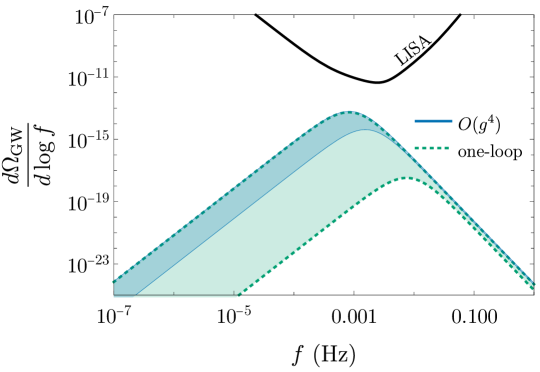
However, Dimensional reduction assumes a hierarchy of scales so that we can integrate out the Matsubara modes. However, for sufficiently strong phase transitions, this hierarchy disappears. For stronger phase transitions, it is plausible that techniques that work in QCD could be repurposed. In particular, numerically solving the Dyson Schwinger equations is a technique that has borne fruit in solving strongly coupled theories Gao et al. (2016). Such a technique has been recently developed for thermal field theory, so far ignoring the momentum dependence of the gap equations Curtin et al. (2018, 2022). A schematic of the current situation is shown in Fig 9 and, as we will see in the next section, simulations do seem to reproduce the above heuristic arguments.

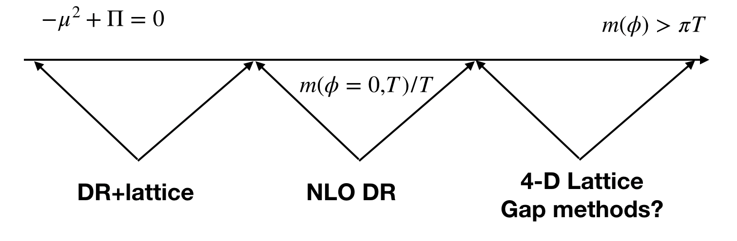
III.6 Simulations

Cosmic phase transitions are such complicated systems, far from equilibrium, that it is necessary to check our analytic methods against simulations. Current numeric results seem to indicate that the theory community has a long way to go in both steps, understanding finite temperature perturbation theory and modeling the gravitational wave spectrum. Recent Monte-Carlo analysis treatments of thermal field theory demonstrated that, in line with expectations, there is indeed a Golilocks zone where perturbation theory yields correct answers when the phase transition is strong enough that infrared catastrophes aren’t numerically important near the critical temperature, yet not so strong that expansions in the coupling constant have slow convergence. However, they found convergence only when expanding in $g^{2}/\lambda$ rather than the traditional expansion in $g^{2}$ , where $g$ is the SU(2) gauge coupling constant and $\lambda$ is the Higgs quartic Gould et al. (2022).

Recent simulations of the sound shell model indicate that the sound shell model overestimates the gravitational wave spectrum due to energy lost to vorticity modes Cutting et al. (2019). Generally, this is a small suppression unless the velocity is small and the trace anomaly large. As for the shape, numerical treatment of the soundshell model does appear to agree fairly well with simulations Hindmarsh et al. (2015, 2017).

The gravitational wave spectrum from scalar shell collisions differs quite dramatically in shape, size, and peak frequency when one compares the predictions of lattice and the envelope approximation Child and Giblin (2012); Cutting et al. (2018, 2021). A significant issue is probably that the contribution to the stress-energy tensor from the bubble wall is ignored after the collision. There has been recent work to try and model this effect and it remains to be seen how much this closes the gap between simulations and theory Jinno and Takimoto (2019); Konstandin (2018); Jinno et al. (2019); Lewicki and Vaskonen (2021); Jinno et al. (2021a); Di et al. (2021).

Of all sources of gravitational waves during a phase transition, our understanding of turbulence is perhaps the most remedial. Recent work considered the gravitational wave background produced a period of freely decay vortical turbulence Auclair et al. (2022). They were able to analytically fit the predicted gravitational wave spectrum, however this eventually needs to matched with a sufficient understanding of how first-order phase transitions source turbulence.

IV Gravitational waves from topological defects

Cosmic phase transitions are not the only source of gravitational waves that can be produced during an event of cosmological symmetry breaking. One possibility is that the vacuum manifold is sufficiently interesting to allow massive configurations of fields that are at least metastable, known as topological defects Kolb and Turner (1990); Vilenkin and Shellard (2000); Maggiore (2018). What makes topological defects a particularly compelling source of gravitational waves is that one does not need to live in a corner of the parameter space to produce such defects. In other words, these topological defects can be formed independently of the order of the phase transition and can generate GWs. This is in contrast to gravitational waves from phase transitions, which require a strong first-order phase transition. Second, and also in contrast to cosmic phase transitions, a gravitational wave signal from such defects can become easier to detect if the scale of physics involved is higher. This is assured directly in the case of cosmic strings as the waveform is relatively flat over many decades of frequency with an amplitude that grows with the symmetry-breaking scale. In the case of domain walls, there is an interplay between the symmetry-breaking scale which determines the power of the gravitational waves emitted, and the lifetime of the wall. In this section, we will give a brief introduction to how to use topology to characterize topological defects, what we know about the gravitational wave signals in the case of each defect as well as hybrids before giving an overview of some recent applications.

IV.1 Categorization by homotopy group

During an epoch of cosmological spontaneous symmetry breaking, if the topology of the vacuum manifold is non-trivial, the transition leaves traces known as topological defects. Depending on the nature of the symmetry under consideration, these defects can be global or local and the phenomenology differs in each case. The full set of possible global or local defects includes domain walls (DW), cosmic strings (CS), monopoles, and textures. To describe the topology of the vacuum manifold, let us use the notation $\mathcal{M}=\mathcal{G}/\mathcal{H}$ , where $\mathcal{G}$ and $\mathcal{H}$ are, respectively, the symmetry groups before and after the symmetry breaking. The topological properties of the manifold, $\mathcal{M}$ , can be diagnosed using homotopy theory. The $n^{\text{th}}$ homotopy group $\Pi_{n}(\mathcal{M})$ classifies qualitatively distinct mapping from the $n-$ dimensional sphere $S^{n}$ into the manifold $\mathcal{M}$ . Below we classify different topological defects based on their vacuum manifold properties and homotopy group,

1.

Domain Walls: They are formed when the vacuum manifolds are disconnected, $i.e~{}\Pi_{0}(\mathcal{M})\neq\mathcal{I}$ , where $\mathcal{I}$ denotes a trivial homotopy group. In other words $\Pi_{0}(\mathcal{M})$ is a homotopy group that counts disconnected components. For example, let us consider a discrete symmetry $Z_{2}$ spontaneously broken to an $\mathcal{I}$ . In this case, the vacuum manifold is given by $\mathcal{M}=Z_{2}/\mathcal{I}$ and $\Pi_{0}(\mathcal{M})=Z_{2}\neq\mathcal{I}$ .
2.

Cosmic strings: CS are formed when the vacuum manifolds are not simply connected, $i.e~{}\Pi_{1}(\mathcal{M})\neq\mathcal{I}$ . Considering a $U(1)$ symmetry that is spontaneously broken to $\mathcal{I}$ , the vacuum manifold can then be written as $\mathcal{M}=U(1)/\mathcal{I}$ and $\Pi_{1}(\mathcal{M})=U(1)\neq\mathcal{I}$ .
3.

Monopoles: These point like defects are formed when $\Pi_{2}(\mathcal{M})\neq\mathcal{I}~{}i.e.$ when the manifold of degenerate vacua contains non-contractible two-surfaces
4.

Textures: Textures appear in the scenarios where the vacuum manifold has a non-trivial third homotopy group, $\Pi_{3}(\mathcal{M})\neq\mathcal{I}$ . For example, if a $O(4)$ is spontaneously broken to $O(3)$ , the vacuum manifold is given by $\mathcal{M}=O(4)/O(3)$ and $\Pi_{3}(\mathcal{M})=O(4)/O(3)\neq\mathcal{I}$ .

IV.2 Gravitational waves from Domain walls

A stochastic GW background can be sourced from different topological defects. As a first example, let us consider domain walls Kolb and Turner (1990); Vilenkin and Shellard (2000); Saikawa (2017). These are sheet-like topological defects that form if a discrete symmetry is spontaneously broken in the early Universe. Once created, their energy density scales inversely with the scale factor. Therefore, they can soon dominate the total energy density of the Universe and later alter the products of BBN as well as the Cosmic microwave background (CMB).

Several solutions exist to overcome domain wall domination Vilenkin and Shellard (2000). For example, if the formation of DW takes place before the inflation, the walls can be inflated away far beyond the present Hubble radius. On the other hand, wall domination can also be avoided in a model where a discrete symmetry that is broken at a very scale is restored at a lower temperature. In this scenario, wall tension (discussed later) is temperature dependent and walls are always over-damped ( $\rho_{\text{DW}}/\rho<<1$ ), hence they never dominate the Universe. Another way out is if the DWs are unstable Vilenkin and Shellard (2000). If domain walls arise from the spontaneous breaking of a global discrete symmetry, one can introduce a small bias to the scalar potential from an explicit symmetry-breaking term that allows the walls to annihilate. Finally, a wall-dominated universe can be avoided if the discrete symmetry responsible for the generation is embedded in a continuous symmetry group and a prior step in the symmetry-breaking chain admits cosmic strings. In such a case, the walls can be bounded by strings and these hybrid defects Vilenkin and Shellard (2000); Dunsky et al. (2022) can decay before they dominate the Universe.

We initiate our discussion by briefly describing the dynamics of DW followed by how it generates the SGWB Saikawa (2017); Huang and Sikivie (1985); Nakayama et al. (2017); Gelmini et al. (2021a); Blasi et al. (2023c, b); Bhattacharya et al. (2023b) that can be detected by the current and future GW detectors. To do that we consider a simplistic scenario of a real scalar field $\phi$ that remains invariant under a discrete $Z_{2}$ symmetry ( $\phi\to-\phi$ ). The $Z_{2}$ symmetry is spontaneously broken, once the scalar obtain a non-zero vacuum expectation value (vev), $i.e.~{}\langle\phi\rangle=\pm v$ . A simple example of such a potential is,

V(\phi)=\frac{\lambda}{4}(\phi^{2}-v^{2})^{2},

(114)

where $\lambda$ is a quartic coupling. Notice, that the scalar has two degenerate minima at $\phi=\pm v$ . As a result of this spontaneous symmetry breaking (SSB), two domains can appear and walls are produced at the boundary. Assuming a static planar doamin wall lying perpendicular to the $x-$ axis in a Minkowski space, $\phi(x)$ , the analytical solution¹²¹²12This solution is only valid when the thickness of wall is smaller than $H^{-1}/\sqrt{2}$ Dolgov et al. (2016). to the equation of motion for this scalar is,

\phi(x)=v~{}\text{tanh}\bigg{(}\sqrt{\frac{\lambda}{2}}vx\bigg{)}.

(115)

Here a local kink is observed at $x=0$ , that takes $\phi$ from $-v$ at $x=-\infty$ to $+v$ at $x=+\infty$ . The surface tension, $\sigma$ , is controlled by the symmetry breaking scale,

\sigma=\int_{\infty}^{\infty}dx\bigg{(}\frac{1}{2}\bigg{[}\frac{\partial\phi(x)}{dx}\bigg{]}^{2}+V(\phi(x))\bigg{)}=\sqrt{\frac{8\lambda}{9}}v^{3}.

(116)

Once the DWs are formed they can eventually dominate the energy budget of the Universe as their energy density dilutes much slower than radiation. Their dynamics can be described by considering them as a system of isotropic gas Vilenkin and Shellard (2000) with an equation of state,

p_{\text{DW}}=\bigg{(}u^{2}-\frac{2}{3}\bigg{)}\rho_{\text{DW}},

(117)

where $p_{\text{DW}}$ and $\rho_{\text{DW}}$ denotes the pressure and energy density of the DWs while $u$ represents the wall’s velocity. While in the case of highly relativistic walls, $u\to 1$ , a usual equation of state for a relativistic gas is obtained $i.e.~{}p_{\text{DW}}=\frac{1}{3}\rho_{\text{DW}}$ , the non-relativistic regime ( $u<<1$ ) gives $i.e.~{}p_{\text{DW}}=-\frac{2}{3}\rho_{\text{DW}}$ . Shortly after forming, the domain walls are expected to have a large mass compared to the background temperature, implying that they will be non-relativistic.

Assuming the Universe to be homogeneous on a scale much greater than the wall separation, it can be approximately described by an FRW metric,

ds^{2}=dt^{2}-a^{2}(t)dx^{2},

(118)

with the equation of state $p=w\rho$ , the scale factor is then given by,

a(t)\propto t^{\frac{2}{3(w+1)}}.

(119)

The DW energy density can then be related to the scale factor as $\rho_{\text{DW}}\propto a^{-3(1+w)}$ . For non-relativistic DWs while $a(t)\propto t^{2}$ , the energy density is $\rho_{\text{DW}}\propto a^{-1}$ . This slow dilution makes a stable domain wall network cosmologically dangerous and conflicting with observation. At this stage it is important to point out that after their formation, the DW dynamics is governed by two different kinds of forces (i) the tension force $p_{\rm T}\sim\sigma/R_{\rm w}$ that helps flatten the wall where $\sigma$ denotes the surface tension and $R_{\rm w}$ represents the curvature radius of the walls, and (ii) friction force $p_{\rm F}\sim vT^{4}$ that appears if the field composing the core of domain wall interacts with the particles in the thermal bath with $v$ being the velocity of DWs. These two forces are balanced $i.e.~{}p_{\rm T}\sim p_{\rm F}$ . Using this condition and replacing $T^{4}\sim M_{\rm Pl}^{2}/t_{r}^{2}$ (assuming the radiation-domination) one can easily show that $\rho_{\rm DW}\propto t_{r}^{-2}$ or $\rho_{\rm DW}\propto a^{-1}$ (as also discussed above) where $t_{r}$ denotes the time when DWs become relativistic. At late times, the friction force is exponentially damped (when the temperature of the radiation bath becomes less than the mass of particles that interact with domain walls). Once $p_{\rm F}$ becomes irrelevant, the DW dynamics is dominated by the tension force $p_{\rm T}$ , which stretches DWs up to the horizon size. Numerical studies Press et al. (1989); Garagounis and Hindmarsh (2003); Oliveira et al. (2005); Avelino et al. (2005); Leite and Martins (2011); Leite et al. (2013); Martins et al. (2016) have shown that the evolution of DW in this regime can be described by the scaling solution. Here, their energy density evolves according to the simple scaling law $\rho_{\rm DW}\propto t^{-1}$ , and their typical size is given by the Hubble radius $\sim t^{2}$ . In the scaling regime, the energy density of the DW can be expressed as,

\displaystyle\rho_{\rm DW}=\sigma\frac{\mathcal{A}}{t},

(120)

with $\mathcal{A}\simeq 0.8\pm 0.1$ being the area parameter Hiramatsu et al. (2014). Even if their energy density is subdominant today, they may still produce excessive density perturbations observable in the CMB epoch if their surface energy density is above $\mathcal{O}(\text{MeV}^{3})$ , this bound is also known as the Zel’dovich-Kobzarev- Okun bound Zeldovich et al. (1974).

As we mentioned, one way to resolve this issue is to make the DWs unstable and allow the network to decay. Let us consider a scenario where the degeneracy of the vacuum is broken by introducing an energy bias in the scalar potential Vilenkin (1981a); Gelmini et al. (1989); Larsson et al. (1997); Bhattacharya et al. (2023b). It is important to point out that, although an energy bias Chiang and Lu (2021); King et al. (2023c); Lu and Chiang (2023); King et al. (2023b) is required to make the DWs unstable, a very large energy difference from the beginning will not allow the formation of DWs at the first place Gelmini et al. (1989). So there must be a hierarchy between the bias terms and the rest of the potential. If the discrete symmetry is approximate, a bias can be established by introducing an explicit symmetry-breaking (in this case $Z_{2}$ ) term Saikawa (2017),

\Delta v(\phi)=\epsilon v\phi\bigg{(}\frac{1}{3}\phi^{2}-v^{2}\bigg{)},

(121)

where $\epsilon$ is a dimensionless constant. Although this potential has a minima at $\pm v$ , there also exists an energy difference between them,

V_{\text{bias}}=V(-v)-V(+v)=\frac{4}{3}\epsilon v^{4}.

(122)

As a result of this energy difference, the false vacuum tends to shrink $i.e.$ there exists a volume pressure force acting on the walls whose magnitude can be estimated as $p_{V}\sim V_{\text{bias}}$ . DW collapses when this pressure force becomes greater than the tension force $p_{T}\sim\sigma\frac{\mathcal{A}}{t}$ . Their annihilation time can be estimated by comparing these two forces,

t_{\text{ann}}=C_{\text{ann}}\frac{\sigma\mathcal{A}}{V_{\text{bias}}},

(123)

where $C_{\text{ann}}$ is a coefficient of $\mathcal{O}(1)$ . Assuming the annihilation occurs in the radiation-dominated era, the temperature at $t=t_{\text{ann}}$ becomes proportional to the inverse square root of Eq. 123,

T_{\rm ann}=3.41\times 10^{-2}\,\mathrm{GeV}\,C_{\rm ann}^{-1/2}\mathcal{A}^{-1/2}\left(\frac{g_{*}(T_{\rm ann})}{10}\right)^{-1/4}\left(\frac{\sigma}{\mathrm{TeV}^{3}}\right)^{-1/2}\left(\frac{V_{\rm bias}}{\mathrm{MeV}^{4}}\right)^{1/2},

(124)

The annihilation of DWs may produce GWs, which are potentially observable today. The Gravitational wave spectrum produced by a DW at cosmic time $t$ can be characterized by the ratio of the rate of change of GW energy density $\rho_{\rm GW}$ with respect to the frequency of the GW $f$ to the critical energy density of the Universe $\rho$ ,

\Omega_{\text{GW}}(t,f)=\frac{1}{\rho_{c}(t)}\frac{d\rho_{\rm GW}(t)}{d\ln f}

(125)

where $\rho_{\rm GW}$ and $f$ denote the energy density and the frequency of the GW respectively. The main feature of the GW spectrum from DW is that it follows a broken power law, where the breaking point has a frequency determined by the annihilation time (when $p_{V}\sim p_{T}$ ) and the peak amplitude is determined by the energy density in the domain walls (which in turn determines the gravitational power radiated). The peak amplitude is therefore dependent upon the fraction of energy radiated into gravitational waves, $\epsilon$ , the surface tension, $\sigma$ , and the radius of the domain wall which is the Hubble radius at the collapse time. Finally, it will depend upon an $\mathcal{O}(1)$ factor $\mathcal{A}$ that captures the precise details of a simulation. Assuming an instantaneous annihilation of the DWs at $t=t_{\rm ann}$ , the peak amplitude is then Saikawa (2017),

\Omega_{\text{GW}}(t_{\rm ann})_{\rm peak}=\frac{1}{\rho_{c}(t_{\rm ann})}\bigg{(}\frac{d\rho_{\rm GW}(t_{\rm ann})}{d\ln f}\bigg{)}_{\rm peak}=\frac{8\pi\tilde{\epsilon}_{\rm GW}G^{2}\mathcal{A}^{2}\sigma^{2}}{3H^{2}(t_{\rm ann})},

(126)

where the parameter $\tilde{\epsilon}_{\rm GW}$ is estimated to be $\tilde{\epsilon}_{\rm GW}\simeq 0.7\pm 0.4$ Hiramatsu et al. (2013) and $G$ is the Newton’s gravitational constant. Once the DWs have entered the scaling regime Avelino et al. (2005), they decay, $i.e$ when their energy density evolves according to the simple scaling law $\rho_{\rm DW}\propto t^{-1}$ , and their size is typically given by the Hubble radius $\sim t$ and hence the peak amplitude at present time $t_{0}$ is,

\Omega_{\text{GW}}h^{2}(t_{0})_{\rm peak}=7.2\times 10^{-18}\tilde{\epsilon}_{\rm GW}\mathcal{A}^{2}\bigg{(}\frac{\sigma}{\rm TeV^{3}}\bigg{)}^{2}\bigg{(}\frac{T_{\rm ann}}{10^{-2}\rm GeV}\bigg{)}^{-4}.

(127)

The redshifted peak frequency can be determined by

	$\displaystyle f_{\rm peak}\simeq\bigg{(}\frac{a(t_{\rm ann})}{a(t_{0})}\bigg{)}H(t_{\rm ann})$		(128)
	$\displaystyle f_{\rm peak}\simeq 1.1\times 10^{-9}~{}{\rm Hz}\bigg{(}\frac{T_{\rm ann}}{10^{-2}\rm GeV}\bigg{)}.$		(129)

To depict the GW spectrum, the following parametrization for a broken power-law spectrum Caprini et al. (2020b); Ferreira et al. (2023) can be adopted

\displaystyle\Omega_{\rm GW}h^{2}=\Omega_{\text{GW}}h^{2}_{\rm peak}\frac{(a+b)^{c}}{\left(bx^{-a/c}+ax^{b/c}\right)^{c}}\ ,

(130)

where $x:=f/f_{p}$ , and $a$ , $b$ and $c$ are real and positive parameters. Here the low-frequency slope $a=3$ can be fixed by causality, while numerical simulations suggest $b\simeq c\simeq 1$ Hiramatsu et al. (2014). While these simulations agree with a scenario where the $Z_{2}$ symmetry is broken, the scenarios with larger discrete symmetries require careful treatment.

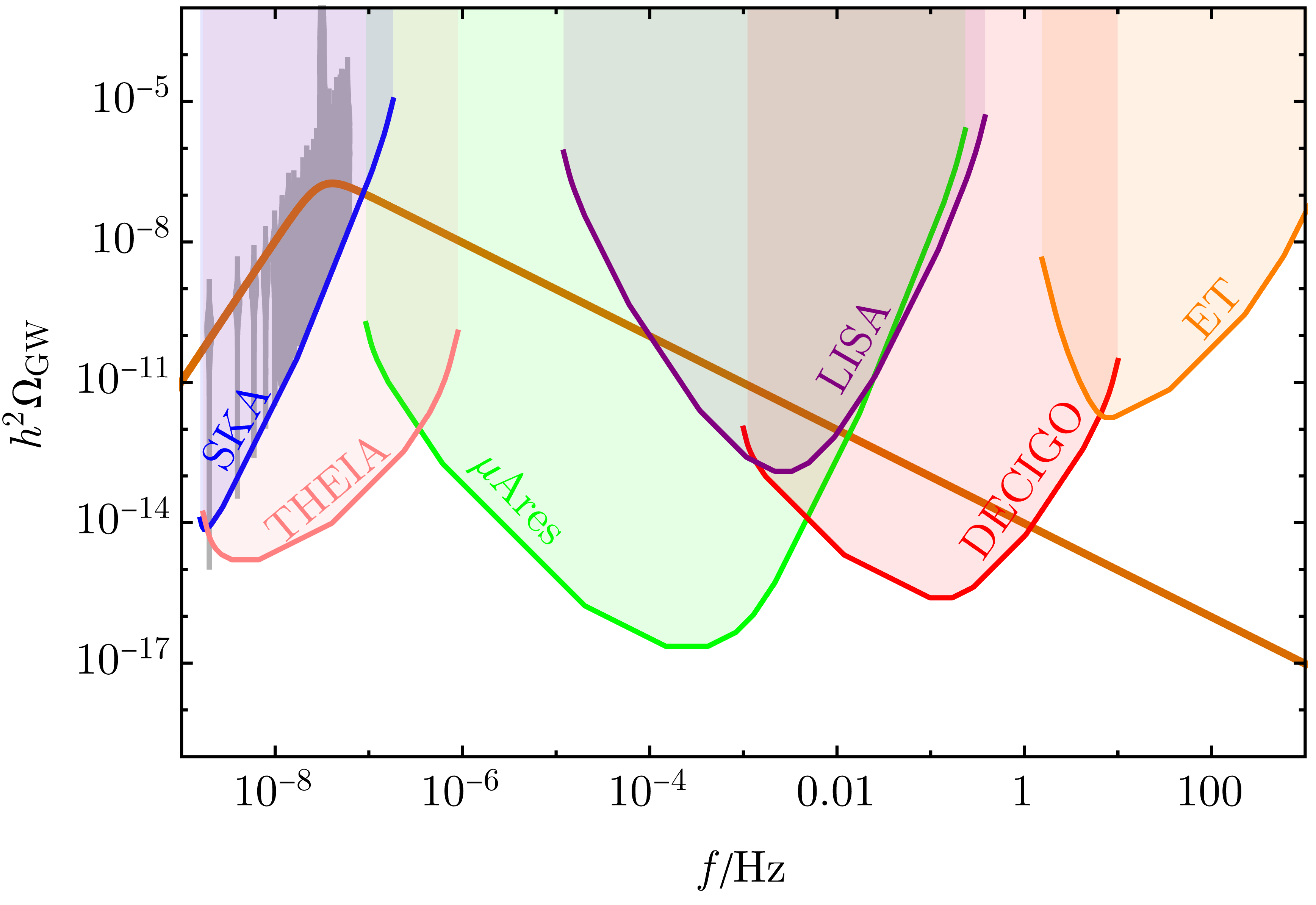
In the case of $Z_{N}$ symmetry for $N>2$ , the UV power law can be modified Hiramatsu et al. (2013); Ferreira et al. (2023); Wu et al. (2022). In this case, multiple degenerate vacua appear, hence leading to a domain wall network that is more complicated to the $Z_{2}$ case. Again, the degeneracy among the vacua can be broken by introducing a bias term in the scalar potential, and eventually, a domain with the lowest energy dominates over others, which causes the annihilation of the walls and the production of GW. It is interesting to point out that GW signals observed in these scenarios can deviate from what is observed in the case of $Z_{2}$ domain walls as also pointed out by a recent study Hiramatsu et al. (2013), that suggests that $b$ in Eq.130 decreases with the increasing value of $N$ .

IV.3 Gravitational waves from Cosmic Strings

Let us now turn our attention to cosmic strings (CS). CSs are one-dimensional defects that appear in many extensions of the SM, e.g., field theories with a spontaneously broken U(1) symmetry (gauge or global) Kibble (1976); Nielsen and Olesen (1973); Vachaspati and Vilenkin (1984); Vilenkin and Shellard (2000); King et al. (2021b); Huang et al. (2020b, a); Lazarides et al. (2021); Maji and Park (2024); Saad (2023); Ahmed et al. (2024); Antusch et al. (2023); Ahmed et al. (2024, 2023, 2022); Afzal et al. (2022), and the fundamental and/or composite strings in superstring theory Copeland et al. (2004); Dvali and Vilenkin (2004); Polchinski (2004); Jackson et al. (2005); Tye et al. (2005). On the other hand, more complicated strings, such as $Z_{N}$ -strings, can also be encountered during the phase transitions followed by a remnant discrete symmetry. For example a $Z_{2}$ string can appear in a GUT model discussed in Kibble et al. (1982b)

SO(10)\longrightarrow SU(5)\times Z_{2}

(131)

In a situation where $N>2$ , $Z_{N}$ -strings can form networks with vertices from which several strings can emerge.

Just like the DWs, once the strings are formed they can also eventually dominate the energy density of the Universe. The effective equation of state for the strings is then given by,

p_{\text{S}}=\bigg{(}\frac{2}{3}u^{2}-\frac{1}{3}\bigg{)}\rho_{\text{S}},

(132)

where $p_{\text{S}}$ and $\rho_{\text{S}}$ denotes the pressure and energy density of the strings while $u$ represents the string’s velocity. For a non-relativistic strings ( $u<<1$ ) gives $i.e.~{}p_{\text{S}}=-\frac{1}{3}\rho_{\text{S}}$ . Following Eq. 119, the CS energy density can then be related to the scale factor as $\rho_{\text{S}}\propto a^{-3(1+w)}$ . For non-relativistic string while $a(t)\propto t$ , the energy density is $\rho_{\text{S}}\propto a^{-2}$ . This suggests that strings can also act as a cosmological disaster. However, the evolution of the string network is much more complicated than this. One should include the two important effects

•

The intercommutation of intersecting string segments leads to the formation of loops of different sizes.
•

The decay of smaller loop by radiating GWs.

At the time of the CS formation, the Universe might have been filled with a surplus amount of strings per horizon. This results from the fact that the correlation length of the field associated with the strings is often much less than the horizon size. Their abundance is then reduced by their self-intersection. String friction with the background plasma, if present, tends to freeze the string on the length scale which is larger than the friction length scale,

R_{\rm fric}=v_{\rm drag}\times t,

(133)

where $v_{\rm drag}$ is the drag speed of the string in the plasma due to friction. This friction retards the rate at which strings reach scaling. However, during this time, strings can still self-intersect and reduce their abundance slowly until typically one string exists per horizon, thereby reaching the scaling regime. At this stage, one string per horizon is maintained as the strings typically intersect whenever

t_{\rm intersect}=L/v_{\rm string}={\rm Hubble\ time}

(134)

is satisfied where $L$ denotes the average inter-string separation scale. This is an attractor solution since the strings will not dilute less than one per horizon since if they dilute a bit more they become superhorizon, and they are stretched as $a(t)\sim t^{1/2}(t^{2/3})$ in the RD (MD) era which is slower than the horizon expansion of $t$ . As a result of this, the horizon always “catches” up with the superhorizon strings as long as the scale factor grows slower than $t$ .

There exist several studies in the literature that have calculated the SGWB from evolving cosmic string networks Hindmarsh (1997); Vincent et al. (1998); Matsunami et al. (2019); Hindmarsh et al. (2021); Blanco-Pillado et al. (2023). Nevertheless, there exists a technical challenge that persists for pure numerical simulation to track the network’s evolution over the entire relevant cosmic history. The issue with the CS network is that at the micro level, we use a field-theoretic treatment. Simulations of the field-theoretic treatment seem to suggest that very limited energy radiated into GW. Once the string is long enough we use a classical Nambu-Goto action string theory treatment. Here, most of the energy is dumped into GWs. It is hard to tell which treatment is right due to the enormous hierarchy of scales involved $i.e.$ inverse string length vs symmetry-breaking scale. Therefore it is difficult to make predictions for observations today. The debate has been ongoing for quite some time, with new insights on both sides of the argument appearing in the last couple of years (see for instance Matsunami et al. (2019); Hindmarsh et al. (2021); Blanco-Pillado et al. (2023)) leaving little confidence that the last word has been uttered.

For the purposes of this review we will proceed with the assumption that the Nambu-Goto treatment is valid. We will use the Velocity-dependent One-Scale (VOS) model Martins and Shellard (1996, 2002) that captures the essential physics, and use it to study and predict the evolution of the string network over a long range of time while calibrating the input model parameters with data points for early time evolution that have been made available by simulations. Next, we briefly review the VOS model.

Following Eq. 125, one can calculate the GW spectrum produced by evolving CS. The idea here is to add up the GW emission from all the loops throughout the history of the Universe. Now, the first basic ingredient for calculating the GW spectrum from the CS is the GW power $P_{\rm GW}$ . The total power emitted in gravitational waves by strings loops can be estimated from the quadrupole formula, $P_{\rm GW}\approx\frac{G}{45}\sum_{i,j}\langle\dddot{Q}_{ij}\dddot{Q}_{ij}\rangle$ . For a string of length $l$ , the quadrupole moment is $Q\sim\mu l^{3}$ where $\mu$ denotes the energy per unit length of a string or the string tension. Now, the oscillation frequency of a relativistically oscillating loop is $\omega\sim 1/l$ , so $\dddot{Q}\sim Q\omega^{3}\sim\mu$ . This gives $P_{\rm GW}\propto G\mu^{2}$ . Note that, since the loop also moves relativistically, one cannot use the quadrupole formula directly. An oscillating string loop of length $l$ emits a discrete set of frequencies $\omega_{n}=2\pi f_{n}$ . Hence, the total power radiated is

\displaystyle P_{\rm GW}=\sum_{n}P_{n},

(135)

where $P_{n}=G\mu^{2}p_{n}$ , so

	$\displaystyle P_{\rm GW}(f,l)=G\mu^{2}\sum_{n}p_{n},$		(136)
	$\displaystyle=G\mu^{2}l\int_{0}^{\infty}dfP(fl),$		(137)

where

\displaystyle P(x)\equiv\sum_{n}p_{n}\delta(x-x_{n}).

(138)

In a continuous limit,

\displaystyle\int_{0}^{\infty}dxP(x)=\Gamma,

(139)

where GW emission efficiency, $\Gamma\sim 50$ Blanco-Pillado et al. (2014); Blanco-Pillado and Olum (2017); Vilenkin (1981b); Blanco-Pillado et al. (2011a) is determined by Nambu-Goto (NG) simulations. Finally, the total power emitted is then expressed as,

\displaystyle P_{\rm GW}=\Gamma G\mu^{2}.

(140)

Following this, the observed energy density of GW at a particular frequency $f$ today is obtained by adding the amount of energy produced at each moment of cosmic evolution for loops of all sizes. Since the $\rho_{\rm GW}$ redshifts as $(a(t)/a_{0})^{-4}$ and hence $\rho_{\rm GW}(t)=(a(t)/a_{0})^{-4}\rho_{\rm GW}(t_{0})$ . On the other hand, the emitted frequency is related to the observed frequency today as $f_{e}=(a(t)/a_{0})^{-1}f_{0}$ , so

\displaystyle\frac{d\rho_{\rm GW}(t)}{df_{e}}=\bigg{(}\frac{a(t)}{a_{0}}\bigg{)}^{-3}\frac{d\rho_{\rm GW}(t_{0})}{df_{0}}.

(141)

Finally, including the result of redshifting, the emission for the moment of emission to today is,

\displaystyle\frac{d\rho_{\rm GW}}{df}(t_{0},f)=G\mu^{2}\int_{0}^{t_{0}}{dt\left(\frac{a(t)}{a_{0}}\right)^{3}\int_{0}^{\infty}{dl~{}l~{}n(l,t)~{}P\left(\frac{a_{0}}{a(t)}fl\right)}}\,,

(142)

where $a(t)$ is the scale factor which takes the value $a_{0}$ today and $n(l,t)$ is the loop number density (see Eq. 145 ). Note that we have just used $f$ to denote $f_{0}$ in Eq. 142.

The second important ingredient for calculating the GW spectrum from the CS is the number density $n(l,t)$ of non-self-intersecting, sub-horizon, CS loops of invariant length $l$ at cosmic time $t$ . To extrapolate the results from simulations (which runs only over a finite time interval) to any moment in the history of the network, the scaling of loops is important as it suggests that,

\displaystyle n(l,t)=t^{-4}n(x),

(143)

where $x=l/t$ is the ratio of the loop size to roughly the horizon scale.

To obtain $n(l,t)$ one approach is to determine the loop production function $\mathbf{f}(l,t)dl$ namely the number density of non-self-intersecting loops of lengths between $l$ and $l+dl$ produced per unit time, per unit volume, which in scaling satisfies,

\displaystyle\mathbf{f}(l,t)=t^{-5}\mathbf{f}(x).

(144)

The loop number density can be obtained by solving the Boltzmann equation for the loops. The Boltzmann equation incorporates the production of loops from the infinite string network as described by $\mathbf{f}(l,t)dl$ , dilution of loops due to the expansion of the Universe, loss of energy through the GWs radiation. The loop number density thus can be calculated by integrating the loop production function Auclair et al. (2020)

\displaystyle n(l,t)=\int_{t_{i}}^{t}{dt^{\prime}\mathbf{f}(l^{\prime},t^{\prime})\left(\frac{a(t^{\prime})}{a(t)}\right)^{3}}\,,

(145)

where the effect of the expansion is explicitly seen through the dependence of the scale factor $a(t)$ , and $l^{\prime}$ (which is given below) contains information on the evolution of the length of the loop due to its gravitational decay from the time of formation $t^{\prime}$ to the observation time $t$ .

Finally, we can relate the loop production function $\mathbf{f}(l,t)$ with the long string network energy density $\rho_{\infty}$ by assuming that the production of loops is the dominant energy loss mechanism of the long string network, which is given by

\displaystyle\frac{d\rho_{\infty}}{dt}=-2H(1+\bar{v}^{2})\rho_{\infty}-\frac{d\rho_{\infty}}{dt}\bigg{|}_{\rm loop}\,,

(146)

where $\bar{v}=\sqrt{\langle v^{2}\rangle}$ is the root-mean-squared (RMS) velocity of the long strings strings. The first term in this equation describes the dilution of the long string energy density in an expanding Universe, while the second, describes energy loss into loop formation. The energy loss in loop formation is proportional to the loop production function, loop length, and string tension,

\displaystyle\frac{d\rho_{\infty}}{dt}\bigg{|}_{\rm loop}\equiv\mu\int_{0}^{\infty}{l\mathbf{f}(l,t)dl}.

(147)

Loop production is essential to achieve the linear scaling of long strings, see e.g. Vilenkin and Shellard (2000).

To determine $n(l,t)$ , it is necessary to have a handle on the evolution of the long string energy density $\rho_{\infty}$ and the root mean velocity $\bar{v}$ of the long string appearing in Eq. 146. To do that one can use the VOS as it describes both the scaling evolution of the long string together with non-scaling evolution through the radiation-matter transition. The evolution can be obtained by solving the coupled differential equations (VOS equation of motion) involving the rate of change of RMS velocity of the long strings and the characteristic length between the strings,

	$\displaystyle\frac{d\bar{v}}{dt}$	$\displaystyle=$	$\displaystyle\left(1-\bar{v}^{2}\right)\left[\frac{k(\bar{v})}{L}-2H\bar{v}\right]\,,$
	$\displaystyle\frac{dL}{dt}$	$\displaystyle=$	$\displaystyle\left(1+\bar{v}^{2}\right)HL+\frac{\tilde{c}}{2}\bar{v}\,,$		(148)

where $L\equiv(\mu/\rho_{\infty})^{1/2}$ denotes the characteristic length that measures the average distance between long strings and $\tilde{c}$ quantifies the efficiency of the loop-chopping mechanism. Note that the second equation of Eq. 148 is nothing but Eq. 146 written in terms of $L$ and $\tilde{c}\bar{v}$ where

\displaystyle\tilde{c}\bar{v}=\mu\frac{L}{\rho_{\infty}}\int_{0}^{\infty}l\mathbf{f}(l,t)dl.

(149)

The function $k(\bar{v})$ accounts for the effects of small-scale structure (namely, multiple kinks) on long strings Martins and Shellard (2002),

\displaystyle k(\bar{v})=\frac{2\sqrt{2}}{\pi}\left(1-\bar{v}^{2}\right)\left(1+2\sqrt{2}\bar{v}^{3}\right)\frac{1-8\bar{v}^{6}}{1+8\bar{v}^{6}}\,,

(150)

This reproduces the expected asymptotic behavior of $k(\bar{v})$ both in the relativistic and non-relativistic limits. The linear scaling of the long string network ( of a form $L=\xi_{s}t$ and $\bar{v}=$ constant Sousa and Avelino (2013a)) in the radiation- and matter-dominated backgrounds follows directly from Eq. 148 since the particular solutions are

\displaystyle\frac{L}{t}=\sqrt{\frac{k(\bar{v})(k(\bar{v})+\tilde{c})}{4\nu(1-\nu)}}\equiv\xi_{s}\qquad\mbox{with}\qquad\bar{v}=\sqrt{\left(\frac{k(\bar{v})}{k(\bar{v})+\tilde{c}}\right)\left(\frac{1-\nu}{\nu}\right)}\equiv\bar{v}_{s}\,,

(151)

where the subscript $s$ stands for ‘scaling’, are attractor solutions of these equations for $a\propto t^{\nu}$ and $0<\nu<1$ with $\xi_{s},\bar{v}_{s}$ being constant. The scaling solution is attainable only for a constant expansion exponent $\nu$ , so, such a regime can only be maintained deep into radiation or matter eras Sousa and Avelino (2013a). More generally, Eq. 148 can be solved throughout any cosmological era, including the radiation-to-matter and matter-to-dark-energy transitions, and hence one can trace the evolution of cosmic string networks in a realistic cosmological background Sousa and Avelino (2013a).

The second step in determining $n(l,t)$ is to relate the loop production function and the long string network as described by the VOS model. Now defining a new variable $\xi\equiv\frac{L(t)}{t}$ which describes the length parameter and as before, $x\equiv\frac{l}{t}$ , it follows from the second equation of Eq. 148 and Eq. 149 that the loop production function satisfies,

\displaystyle\int_{0}^{\infty}{x\mathbf{f}(x)~{}dx}=\frac{2}{\xi^{2}}\left[1-\nu(1+\bar{v}^{2})\right]=\tilde{c}\frac{\bar{v}}{\xi^{3}}\equiv C_{\rm eff}\,.

(152)

Now, one can make the following assumption¹³¹³13There exist two other models to calculate the loop number density. In the first one Blanco-Pillado et al. (2011b, 2014); Auclair et al. (2020) one can use loop production functions for non-self-intersecting loops directly from NG simulations of cosmic string and in the second one Lorenz et al. (2010); Ringeval et al. (2007); Auclair et al. (2020) the loop production function is not the quantity inferred from the simulation but the distribution of non-self-intersecting scaling loops is directly extracted from the simulation. throughout cosmic history, all loops are assumed to be created with a length $l$ that is a fixed fraction of the characteristic length of the long string network, namely $l=\alpha_{L}L$ , with $\alpha_{L}<1$ . Thus

\displaystyle\mathbf{f}(x)={\tilde{C}}\delta\left(x-\alpha_{L}\xi\right).

(153)

From Eq. (152) we obtain,

\displaystyle\tilde{C}=\frac{\tilde{c}}{\alpha_{L}}\frac{\bar{v}}{\xi^{4}}\,

(154)

with $\bar{v}$ and $\xi=L/t$ being the solutions of the VOS Eq. 148. Note that the value of $\tilde{C}$ in the above equation is an upper limit since Eq. 152 does not carry the information that some of the energy of the long string network goes redshifting of the peculiar velocities of loops. Introducing $f_{r}\sim\sqrt{2}$ which denotes the reduction factor that accounts for the energy loss into redshifting of the peculiar velocities of loops and $\mathcal{F}$ that denotes the fraction of loops formed with size $\alpha_{L}$ as not all the loops created need to be of the same size. Taking these corrections into account, the loop production function can be written as

\displaystyle\mathbf{f}(x)=\left(\frac{\mathcal{F}}{f_{r}}\right){\tilde{C}}\delta\left(x-\alpha_{L}\xi\right)\equiv A~{}\delta\left(x-\alpha_{L}\xi\right)\,,

(155)

This expression is valid throughout cosmic history, even when the cosmic string network is not in a linear scaling regime (in this case $x$ and $\tilde{C}$ will be time-dependent).

Finally, substituting Eq. 155 in Eq. 145 one can obtain loop number density for all times including during the radiation-to-matter and matter-to-dark-energy transitions but this requires solving the VOS equation of motion. During the radiation era ( $\nu=1/2$ ), the long string network is scaling and described by the VOS solutions (Eq. 151), namely $\xi_{r}=0.271$ and $v_{r}=0.662$ , hence it follows that the loop distribution takes a simple form

\displaystyle n_{r}(x)=\frac{A_{r}}{\alpha}\frac{\left(\alpha+\mathrm{\Gamma}G\mu\right)^{3/2}}{\left(x+\mathrm{\Gamma}G\mu\right)^{5/2}}\,,

(156)

with $A_{r}=0.54$ (fixing ${\cal F}=0.1$ ), and where $\alpha=\alpha_{L}\xi_{r}$ . As noted above, this expression is only valid for $x\leq\alpha$ . In a matter-only universe ( $\nu=2/3$ ), the VOS scaling solutions (Eq. 151) give $\xi_{m}=0.625$ and $v_{m}=0.583$ and the loop distribution is

\displaystyle n_{m}(x)=\frac{A_{m}}{\alpha_{m}}\frac{\alpha_{m}+\mathrm{\Gamma}G\mu}{\left(x+\mathrm{\Gamma}G\mu\right)^{2}}\,,

(157)

where $\alpha_{m}=\alpha_{L}\xi_{m}$ , $A_{m}=0.039$ and $x\leq\alpha_{m}$ .

We are now at a point where we must take divergent paths - the evolution of the string network is qualitatively different if the strings arise from a global or a local symmetry. We will refer to each case as a global and local string network respectively and separately describe their evolution including the above effects.

IV.3.1 Cosmic strings from global $U(1)$ symmetry breaking

Let us first consider the case of global strings. Although we will introduce some key concepts that are common for both global as well as local strings. We will consider a simple setup with a global $U(1)$ symmetry that is spontaneously broken by a complex scalar $\phi$ . The model features global strings that result from this breaking. The setup can be described by the Lagrangian,

	$\displaystyle\mathcal{L}=\partial_{\mu}\phi^{*}\partial^{\mu}\phi-V(\phi),$		(158)
	$\displaystyle V(\phi)=\frac{1}{2}\lambda(\|\phi\|^{2}-\frac{1}{2}\eta^{2})^{2},$		(159)

where $\eta$ denotes the vacuum expectation value of $\phi$ . This spontaneous breaking of global $U(1)$ also leads to the formation of a massless Nambu-Goldstone boson. Depending on the magnitude of $\eta$ , these global strings can either decay dominantly to the Goldstone bosons or the GWs (see the discussion below Eq. 160 ). In this scenario, the GWs are mostly suppressed and their amplitude mildly falls with frequency for most of the spectrum of interest. Although, this makes their detection a bit difficult, works like Chang and Cui (2020, 2022); Di Bari et al. (2023); Gorghetto et al. (2021) suggest that they can still be detected by GW experiments like LISA, AEDGE, DECIGO, and BBO by considering the breaking scale $\eta$ above $10^{14}$ GeV.

Once formed, the loop oscillates and emits its energy in the form of Goldstone (first term) and gravitational waves (second term) as shown in the equation below Vilenkin and Vachaspati (1987)

\displaystyle\frac{dE}{dt}=-\Gamma_{a}\eta^{2}-\Gamma G\mu^{2},.

(160)

The parameter $\Gamma_{(a)}$ depends only on the loop trajectory Vilenkin and Shellard (2000); Battye and Shellard (1997), and hence we expect that the value of the Goldstone radiation constant $\Gamma_{a}$ must be close to the value of the GW radiation constant $\Gamma\sim\Gamma_{a}$ Battye and Shellard (1997). The Goldstone radiation constant is found to be $\Gamma_{a}\sim 65$ Vilenkin and Shellard (2000); Battye and Shellard (1997). The absence of the gauge field in the breaking of the global $U(1)$ symmetry implies the presence of Goldstone (as discussed earlier) with logarithmically divergent gradient energy,

\displaystyle\mu(t)=2\pi\eta^{2}\log{\frac{L(t)}{\delta}},

(161)

The string tension depends on the ratio of two scales, a macroscopic scale $L(t)$ (close to the Hubble scale), and a microscopic scale $\delta(t)\propto 1/\eta$ representing the width of the string core. It is interesting to point out that even though the $\Gamma_{(a)}$ are similar in size, the GW radiation has a relative suppression of $\eta^{2}/M_{\rm p}^{2}$ . However, this suppression becomes less severe once the symmetry-breaking scale $\eta$ gets closer to $M_{\rm p}$ . For this reason, next-generation gravitational wave detectors are only sensitive to global strings formed during symmetry breaking occurring near the GUT scale. Due to the emission of the Goldstones together with the GW, a loop of initial length $\ell_{i}=\alpha t_{i}$ at a later time reduces,

\displaystyle\ell(t)\simeq\alpha t_{i}-\Gamma G\mu(t-t_{i})-\frac{\Gamma_{a}}{2\pi}\frac{t-t_{i}}{\log{\frac{L(t)}{\delta}}},.

(162)

where the second and third terms denote the decrease in loop size for gravitational wave emission and Goldstone emission, respectively.

A string loop emits the Goldstone and the GW from normal mode oscillations with frequencies Vachaspati and Vilenkin (1985a); Allen and Shellard (1992); Maggiore (2018),

\displaystyle\tilde{f}_{k}=2k/\tilde{l},

(163)

where $k=1,2,3,\ldots$ , and $\tilde{l}\equiv l(\tilde{t})$ is the instantaneous size of a loop when it radiates at $\tilde{t}$ . The distribution of power in the different harmonics is determined by the small-scale structure of the loops. It was shown Vachaspati and Vilenkin (1985a); Allen and Shellard (1992) that, in the large $k$ limit, the power emitted in each mode scales as $k^{-4/3}$ if the loop contains points where the velocity is locally 1 known as cusps; as $k^{-5/3}$ , if it has kinks (which are discontinuities in the tangential vector introduced by the intercommutation process); and $k^{-2}$ when kink-kink collisions occur. In principle, when computing the SGWB generated by cosmic string loops, one should consider the contribution of all the harmonic modes of emission. The radiation parameters can be decomposed as $\Gamma=\sum_{k}\Gamma^{(k)}$ and $\Gamma_{a}=\sum_{k}\Gamma_{a}^{(k)}$ , with

\displaystyle\Gamma^{(k)}=\frac{\Gamma k^{-n}}{\sum_{j=1}^{\infty}j^{-n}},\quad\text{and\quad}\Gamma_{a}^{(k)}=\frac{\Gamma_{a}k^{-n}}{\sum_{j=1}^{\infty}j^{-n}},

(164)

and the normalization factor is approximately $\sum_{j=1}^{\infty}j^{-4/3}\simeq 3.60$ .

Taking into account the redshifted frequency $f_{k}=\frac{a(\tilde{t})}{a(t_{0})}\tilde{f}_{k}$ , with $t_{0}$ denoting the present time and $a(t_{0})\equiv 1$ being scale factor today, the gravitational wave amplitude is summed over all normal modes

\displaystyle\Omega_{\rm GW}(f)=\sum_{k}\Omega_{\rm GW}^{(k)}(f)=\sum\frac{1}{\rho_{c}}\frac{d\rho_{\rm GW}}{d\log{f_{k}}}.

(165)

Now, the contribution from an individual $k$ mode can be obtained by taking an integral over the evolving number density,

	$\displaystyle\Omega_{\rm GW}^{(k)}(f)=\frac{\mathcal{F}_{\alpha}F_{a}}{\alpha\rho_{c}}\frac{2k}{f}\int_{t_{f}}^{t_{0}}d\tilde{t}\frac{C_{\rm eff}\left(t_{i}^{(k)}\right)}{t_{i}^{(k)4}}\frac{\Gamma^{(k)}G\mu^{2}}{\alpha+\Gamma G\mu+\frac{\Gamma_{a}}{2\pi\frac{L(t)}{\delta}}}\left[\frac{a(\tilde{t})}{a(t_{0})}\right]^{5}\left[\frac{a\left(t_{i}^{(k)}\right)}{a(\tilde{t})}\right]^{3}\theta(\tilde{\ell})\theta(\tilde{t}-t_{i}),$
			(166)

while $t_{f}$ denotes the time of network formation, the first Heaviside theta functions guarantee causality (i.e the size of the source is limited to the horizon size), and the second Heaviside theta function suggests that the GWs are only emitted once the loops are formed. Following Eq. 162, one can easily find that a loop that emits GW at time $\tilde{t}$ leading to an observed frequency $f$ was formed at the time

\displaystyle t_{i}^{(k)}=\frac{\tilde{\ell}(\tilde{t},f,k)+\left(\Gamma G\mu+\frac{\Gamma_{a}}{2\pi\frac{L(t)}{\delta}}\right)\tilde{t}}{\alpha+\Gamma G\mu+\frac{\Gamma_{a}}{2\pi\frac{L(t)}{\delta}}},

(167)

where the loop size can be written as $\tilde{\ell}=2ka(\tilde{t})/f$ .

The GW spectrum can be divided into three regions. The spectrum in these three region can be approximated by Chang and Cui (2022)

{\Omega_{\rm GW}(f)h^{2}}\simeq\left\{\begin{array}[]{cc}5.1\times 10^{-15}\left(\frac{\eta}{10^{15}{\rm GeV}}\right)^{4}\left(\frac{f}{f_{\eta}}\right)^{-1/3},&{\rm for}~{}f_{\eta}<f\\ 8.8\times 10^{-18}\left(\frac{\eta}{10^{15}{\rm GeV}}\right)^{4}\log^{3}\left[\left(\frac{2}{\alpha f}\right)^{2}\frac{\eta}{t_{\rm eq}}\frac{1}{z_{\rm eq}^{2}\sqrt{\xi}}\Delta_{R}^{1/2}(f)\right]\Delta_{R}(f),&{\rm for}~{}f_{\rm eq}<f<f_{\eta}\\ 2.9\times 10^{-12}\left(\frac{\eta}{10^{15}{\rm GeV}}\right)^{4}\left(\frac{f}{f_{\rm eq}}\right)^{-1/3},&{\rm for}~{}f_{0}<f<f_{\rm eq}\\ 0,&{\rm for}~{}f<f_{0}\end{array}\right.

(168)

where $t_{\rm eq}$ and $z_{\rm eq}$ are the time and red-shift at the epoch of matter-radiation equality, $\Delta_{R}(f)$ takes care of the effect of varying the number of relativistic degrees of freedom, $g_{\star}$ and $g_{\star S}$ , over time

\displaystyle\Delta_{R}(f)=\frac{g_{\star}(f)}{g_{\star}^{0}}\bigg{(}\frac{g_{\star S}^{0}}{g_{\star S}(f)}\bigg{)}^{4/3},

(169)

with superscript $0$ denoting the values at present times. In the first region where the frequency is very high, $f_{\eta}<f$ Battye and Shellard (1996), the signal falls off, and the exact shape depends on the initial conditions and very early stages of the string network evolution not fully captured by the VOS model Martins and Shellard (1996, 2002); Martins et al. (2004); Martins and Cabral (2016); Martins (2019); Correia and Martins (2019) discussed above. $f_{\eta}$ is related to the time when the Goldstone radiation becomes significant. The radiation-dominated era that corresponds to the second region, $f_{\rm eq}<f<f_{\eta}$ , the spectrum fall as $~{}\log^{3}{(1/f)}$ . $f_{\rm eq}$ indicates the frequency corresponding to the emission around the time of matter-radiation equality. Finally, in the last region that corresponds to the matter-domination $f_{0}<f<f_{\rm eq}$ , the spectrum falls as $f^{-1/3}$ . $f_{\rm eq}$ is related to the time of matter-radiation equality, and $f_{0}$ is related to the emission at the present time. These characteristic frequencies are given by

$\displaystyle f_{\eta}$	$\displaystyle\sim\frac{2}{\alpha t_{n}}\frac{a(t_{\eta})}{a(t_{0})}\sim 10^{10}\ \text{Hz},$	(170)
$\displaystyle f_{0}$	$\displaystyle\sim\frac{2}{\alpha t_{0}}\sim 3.6\times 10^{-16}\ \text{Hz},$	(171)
$\displaystyle f_{\rm eq}$	$\displaystyle\sim 1.8\times 10^{-7}\ \text{Hz}.$	(172)

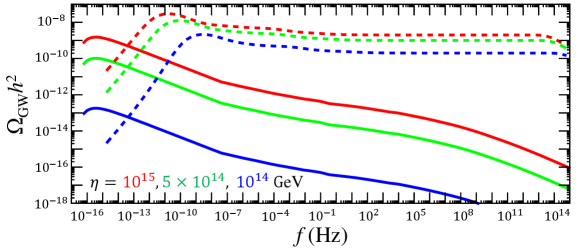
IV.3.2 Cosmic strings from gauged $U(1)$ symmetry breaking

Unlike global strings, local strings or the Nambu-Goto strings are formed by gauging a $U(1)$ symmetry. In this scenario, the Goldstones are eaten by $U(1)$ vector bosons. Once formed, these Nambu-Goto strings radiate their energy primarily via loop generation and emission of GW which has a flat spectrum Gouttenoire et al. (2020); Lazarides et al. (2022b); Borah et al. (2022); Lazarides et al. (2022a); Borah et al. (2023). $10\%$ of the loops formed are large and the remaining are highly boosted smaller loops Vanchurin et al. (2006); Martins and Shellard (2006); Olum and Vanchurin (2007); Ringeval et al. (2007); Blanco-Pillado and Olum (2017). The loop formation from the long strings can again be described using the VOS model. Contrary to the case of global strings where energy per unit length, $\mu$ has a logarithmic dependence (see Eq. 161), the energy is radiated at a constant rate during the oscillation of the larger loops for Nambu-Goto strings as $\mu$ remains constant,

\displaystyle\frac{dE}{dt}=-\Gamma G\mu^{2}.

(173)

In general, for local strings $\mu\sim\mathcal{O}(\eta)$ . Since there is no emission of Goldstone, Eq. 162 can now be written as,

\displaystyle\l(t)\simeq\alpha t_{i}-\Gamma G\mu(t-t_{i}).

(174)

Integrating over the emission time, the gravitational wave amplitude of the $k$ -th mode is given by

\displaystyle\Omega_{\rm GW}^{(k)}(f)=\frac{1}{\rho_{c}}\frac{2k}{f}\frac{\mathcal{F}_{\alpha}\Gamma^{(k)}G\mu^{2}}{\alpha(\alpha+\Gamma G\mu)}\int_{t_{F}}^{t_{0}}d\tilde{t}\frac{C_{\rm eff}(t_{i}^{(k)})}{{t_{i}^{(k)}}^{4}}\left[\frac{a(\tilde{t})}{a(t_{0})}\right]^{5}\left[\frac{a(t_{i}^{(k)})}{a(\tilde{t})}\right]^{3}\ \Theta(t_{i}^{(k)}-t_{F})\,,

(175)

where $\Gamma^{(k)}$ can be obtained from Eq. 164, $t_{i}^{(k)}$ is the formation time of loops contributing to the $k$ -th mode and is given by

\displaystyle t_{i}^{(k)}(\tilde{t},f)=\frac{1}{\alpha+\Gamma G\mu}\left[\frac{2k}{f}\frac{a(\tilde{t})}{a(t_{0})}+\Gamma G\mu\tilde{t}\right].

(176)

Summing over all modes, we get the total amplitude of the gravitational waves

\displaystyle\Omega_{\rm GW}(f)=\sum_{k}\Omega_{\rm GW}^{(k)}(f)\,,

(177)

where the sum can be easily evaluated using

\displaystyle\Omega_{\rm GW}^{(k)}(f)=\frac{\Gamma^{(k)}}{\Gamma^{(1)}}\Omega_{\rm GW}^{(1)}(f/k)=k^{-4/3}\ \Omega_{\rm GW}^{(1)}(f/k)\,.

(178)

A typical shape of a GW signal generated by Nambu-Goto strings is a rising spectrum at a low frequency and thereafter a plateau is observed at higher frequencies. The height of the plateau is proportional to the symmetry-breaking scale $\eta$ . This gentle dependence (linear) of $\Omega$ on $\eta$ in Fig. 11 means next-generation detectors can probe a large range of symmetry-breaking scales.

IV.4 Gravitational waves from Monopoles and Textures

Monopoles or localized defects are point-like defects that arise from the SSB of some larger spherical symmetry. The existence of a monopole solution was first discussed by ’t Hooft and Polyakov in a gauge $SO(3)$ model with a scalar triplet field. The setup can be described by the Lagrangian,

{\cal L}=\frac{1}{2}D^{\mu}\phi D_{\mu}\phi-\frac{1}{4}B_{\mu\nu}B^{\mu\nu}-\frac{\lambda}{4}\left(\phi^{2}-v^{2}_{\phi}\right)^{2}\ .

(179)

where $\phi$ is a scalar triplet. The ‘t Hooft-Polyakov monopole ’t Hooft (1974); Polyakov (1974) has the solution

$\displaystyle\phi$	$\displaystyle=$	$\displaystyle\hat{r}\frac{h(v_{\phi}er)}{er}$
$\displaystyle W^{i}_{a}$	$\displaystyle=$	$\displaystyle\epsilon_{aij}\hat{x}^{j}\frac{1-f(v_{\phi}er)}{er}$
$\displaystyle W_{a}^{0}$	$\displaystyle=$	$\displaystyle 0\,,$	(180)

where, using the shorthand $\xi=v_{\phi}er$ for the product of $v_{\phi}$ with the gauge coupling constant $e$ and radial coordinate $r$ , the functions $f$ and $h$ are solutions to the equations ’t Hooft (1974); Polyakov (1974).

	$\displaystyle\xi^{2}\frac{d^{2}f}{d\xi^{2}}$	$\displaystyle=$	$\displaystyle f(\xi)h(\xi)^{2}+f(\xi)(f(\xi)^{2}-1)$		(181)
	$\displaystyle\xi^{2}\frac{d^{2}h}{d\xi^{2}}$	$\displaystyle=$	$\displaystyle 2f(\xi)^{2}h(\xi)+\frac{\lambda}{e^{2}}h(\xi)(h(\xi)^{2}-\xi^{2})\ .$		(182)

The boundary conditions satisfy $\lim_{\xi\to 0}f(\xi)-1=\lim_{\xi\to 0}h(\xi)\sim{\cal O}(\xi)$ and $\lim_{\xi\to\infty}f(\xi)=0$ , $\lim_{\xi\to\infty}h(\xi)\sim\xi$ . The monopole mass again comes from solving the equations of motion and then calculating the static Hamiltonian,

	$\displaystyle E=m$	$\displaystyle=$	$\displaystyle\frac{4\pi v_{\phi}}{e}\int_{0}^{\infty}\frac{d\xi}{\xi^{2}}\left[\xi^{2}\left(\frac{df}{d\xi}\right)^{2}+\frac{1}{2}\left(\xi\frac{dh}{d\xi}-h\right)^{2}\right.$		(183)
			$\displaystyle\left.+\frac{1}{2}(f^{2}-1)^{2}+f^{2}h^{2}+\frac{\lambda}{4e^{2}}(h^{2}-\xi^{2})^{2}\right]\ .$		(183)

It has the form

m=\frac{4\pi v_{\phi}}{e}f(\lambda/e^{2})\ .

(184)

The solution has been calculated numerically for multiple values, and one finds that for $0.1<\lambda/e^{2}<10^{1}$ , $f(\lambda/e^{2})$ is slowly varying ${\cal O}(1)$ function ’t Hooft (1974).

It is well known that monopoles with an initial abundance of roughly one per horizon at formation as computed by Kibble Kibble (1976), have no gravitational wave amplitude. Following the Kibble-Zurek mechanism Zurek (1985), it was recently shown in Dunsky et al. (2022) that a relativistic monopole-bounded string network can emit a pulse of GW before decaying assuming the friction is low. Such a scenario falls under the category of hybrid defects and is discussed in section IV.5.

Textures, on the other hand, are defects in three spatial directions Vilenkin and Shellard (2000). Sometimes they are also referred to as non-singular soliton, as the scalar field is nowhere topologically constrained to rise from the minimum of the scalar potential. They can arise either from the breaking of a global symmetry or the breaking of a gauge symmetry. After their formation, the global texture releases their energy during their collapse in the form of Goldstone bosons and GWs. It produces a flat spectrum with its peak amplitude controlled by the symmetry-breaking scale $i.e.~{}\Omega_{\rm{GW}}h^{2}\sim v^{4}$ , where $v$ is the breaking scale of global symmetry. The produced gravitational wave spectrum is scale-invariant as the amplitude does not depend on the frequency. There is no dependence on the self-coupling of the symmetry-breaking field. This is because the effective theory of the Goldstone modes, responsible for the creation of the GWs, is a nonlinear $\sigma$ model, and the coupling disappears when the scalar field mode is integrated out Durrer et al. (1999); Figueroa et al. (2013); Fenu et al. (2009). On the other hand, gauged textures also can generate GW once produced from the breaking of local symmetry. The GW generated from the gauged texture is not scale invariant, this is because the gauge field configuration cancels the gradient of the scalar field on the large scale. In this case, there exists a cutoff on the spectrum $f_{0}\sim 10^{11}~{}\rm{Hz}$ Dror et al. (2020). To test the GW generated from the gauged textures one requires future GW experiments that are sensitive to a very high frequency.

IV.5 Hybrid defects

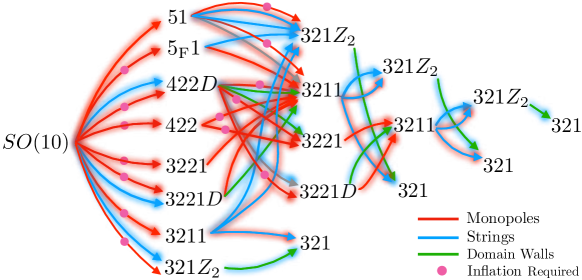
Hybrid defects Langacker and Pi (1980); Lazarides et al. (1982); Vilenkin (1982); Vilenkin and Shellard (2000); Dunsky et al. (2022); Buchmuller et al. (2023) are generated due to a chain of symmetry breaking events, $\mathcal{G}\to\mathcal{H}\to\mathcal{K}$ , where the defects of different dimensionalities get clubbed together. For example, a Hybrid effect can be generated where cosmic strings are attached to DWs or monopoles are attached to a string. Such hybrid defects are generally unstable with one defect eating the other via the conversion of its rest mass into the other’s kinetic energy. The leftover defect decays further resulting in the production of GW. For the purpose of demonstration, we show a simple schematic of $SO(10)$ symmetry breaking chain to SM that produces hybrid defects in Fig. 12, the figure is taken from Dunsky et al. (2022). We now, briefly summarize some of these hybrid defects and the GW spectrum generated as a result of their collapse. It was proven in ref. Dunsky et al. (2022) that if a defect involving an $n$ dimensional object appears in the first symmetry breaking step, any defects from the next symmetry breaking step must have a dimension lower than $n$ , so we can write the full list of possible hybrid defects as follows,

•

String-Monopole network: The hybrid defects associated with the string-monopole system Langacker and Pi (1980); Lazarides et al. (1982); Vilenkin (1982); Dunsky et al. (2022); Buchmuller et al. (2023); Lazarides et al. (2023, 2022c) can be categorized by either monopoles nucleating and eating a string network or strings attaching to and eating a preexisting monopole network. In the first case, a vacuum manifold $\mathcal{H}/\mathcal{K}$ is not simply connected to a full vacuum manifold $\mathcal{G}/\mathcal{K}$ . Then $\pi_{1}(\mathcal{H}/\mathcal{K})\neq I$ results in the formation of topologically unstable strings that manifest themselves by nucleation of magnetic monopole pairs that eat the strings. Such kinds of monopoles must always arise from the earlier phase transition $\mathcal{G}/\mathcal{H}$ (generally before inflation) so that $\pi_{2}(\mathcal{G}/\mathcal{H})\neq I$ . Consider a scenario where in the first phase a spherical symmetry (non-abelian gauge group) is broken to a $U(1)$ leading to a formation of monopoles, and in the second phase when $U(1)$ is broken, strings are formed. If the $U(1)$ symmetry involved in the production of monopoles partially overlaps or coincides with the $U(1)$ symmetry responsible for the string formation, the strings become metastable as monopoles-antimonopole pairs nucleate along the strings (see Fig. 13) through Schwinger nucleation by quantum tunneling. Conversion of the string’s rest mass into the monopole’s kinetic energy leads to relativistic oscillations of the monopoles before the system collapses via radiating GW and monopole annihilations Martin and Vilenkin (1997); Leblond et al. (2009); Dunsky et al. (2022); Buchmuller et al. (2021); Afzal et al. (2022, 2023a); Ahmed et al. (2024); Antusch et al. (2023); Lazarides et al. (2022c, 2023).

The total power emitted in the form of GW by string loops before nucleation or by the relativistic monopoles post-nucleation can be calculated using the gravitational power as given in Eq. 140. The power emitted by the string loops or monopole-bounded strings should be comparable since the kinetic energy of the relativistic monopoles originates from the rest mass of the string. Here, $\Gamma\approx 50$ for string loops before nucleation and $\Gamma\approx 4\ln\gamma_{0}^{2}$ for relativistic monopoles bounded to strings post-nucleation Leblond et al. (2009), whereas $\gamma_{0}\approx 1+\mu l/2m$ is the monopole Lorentz factor arising from the conversion of string rest mass energy to monopole kinetic energy. The power emitted by gravitational waves reduces the string length (see Eq. 174) with a loop lifetime of order $\alpha t_{i}/\Gamma G\mu$ . The string length ( $l$ ) and harmonic number $n$ is set by the emission frequency, $f^{\prime}=n/T=2n/l$ , where $T=l/2$ is the period of any string loop Weinberg (1972); Vilenkin and Shellard (2000). The redshifted frequency observed today is,

f=\frac{2n}{l}\frac{a(t_{0})}{a(t)},

(185)

where $t_{0}$ is the present time.

The number density spectrum of string loops is as before but modified by a term that captures the rate of cutting strings by monopoles,

	$\displaystyle\mathcal{N}(l,t)_{\rm Schwinger}$	$\displaystyle\equiv\frac{dn}{dl}(l,t)\approx\frac{dn}{dt_{i}}\frac{dt_{i}}{dl}e^{-\Gamma_{m}l(t-t_{i})}$			(186)
		$\displaystyle=\frac{\mathcal{F}C_{\rm eff}(t_{i})}{t_{i}^{4}\alpha(\alpha+\Gamma G\mu)}\Bigl{(}\frac{a(t_{i})}{a(t)}\Bigr{)}^{3}e^{-\Gamma_{m}l(t-t_{i})},$			(186)

where the tunneling rate per unit string length can be estimated from the bounce action formalism Kibble et al. (1982a); Preskill and Vilenkin (1993) and is exponentially suppressed by powers of the ratio of the symmetry breaking scales Leblond et al. (2009)

\Gamma_{m}=\frac{\mu}{2\pi}{\rm exp}(-\pi\kappa_{m})\ ,

(187)

with $\kappa_{m}=m^{2}/\mu$ . Typically, $m\sim v_{m}$ and $\mu\sim v_{\mu}^{2}$ where $v_{\mu}$ ( $v_{m}$ ) is the breaking scale that leads to the formation of CS (monopole). To get a GW signal in this situation, one needs to have $v_{m}\sim v_{\mu}$ so that $\kappa_{m}$ is not extremely large otherwise the GW spectrum remains identical to the standard stochastic string spectrum as the string remains stable for a larger value of $\kappa_{m}$ . Going back to Eq. 186, the exponential factor on the right side of Eq. 186 is the monopole nucleation probability. This effectively cuts off loop production and destroys the loops with a length large enough to nucleate with significant probability. The probability of nucleation is negligible and the string network evolves like a standard, stable string network for $\Gamma_{m}l(t-t_{i})\ll 1$ . Note that this cutoff is time-dependent,

\Gamma_{m}\,l(t-t_{i})=\Gamma_{m}\frac{2n}{f}\frac{a(t)}{a(t_{0})}(t-t_{i})\ .

(188)

Following Eq. 186 one finds that even though the number density of string loops decreases when nucleation occurs (exponential suppression), the number density of string-bounded monopoles still increases. A loop that nucleates monopoles will continue to nucleate and fragment into many monopole-bounded strings for $l_{\rm max}\gg l_{\rm tp}$ , with size of order $l\sim l_{\rm tp}\ll l_{\rm max}$ with $l_{\rm tp}$ denoting the critical length above which it is energetically favorable for the string to form a gap of length $l_{\rm tp}$ , separating two monopole endpoints and $l_{\rm max}$ denotes the maximum string size. In this situation, the net energy density eventually deposited into gravitational waves is much less even if the the total energy density in these pieces is comparable to the original energy density of the parent string loop. This can be understood in the following manner, the lifetime of the string-bounded monopoles $\sim\mu l_{\rm tp}/\Gamma G\mu^{2}$ is much smaller than the parent loop because their power emitted in gravitational waves is similar to pure loops while their mass is much smaller. The net energy density that is transferred into gravitational waves is, to a good approximation, the energy density of the defect at the time of decay. Since these pieces decay quickly and do not redshift $\propto a^{3}$ for as long as pure string loops, their relative energy density compared to the background at their time of decay is much less than for pure string loops. As a result, the net energy density that goes into gravitational radiation by monopole-bounded string pieces compared to string loops is small, and hence their contribution to the spectrum can be neglected.

The gravitational wave energy density spectrum generated from a network of metastable cosmic strings, including dilution and redshifting due to the expansion history of the Universe can be obtained using Eq. 142 and replacing,

\frac{dn}{dl}(l,t^{\prime})=\mathcal{N}(l,t^{\prime})_{\rm Schwinger},~{}\\ ~{}\text{and}\frac{dP(l,t^{\prime})}{df^{\prime}}=\Gamma G\mu^{2}l\,g\left(f\frac{a(t)}{a(t^{\prime})}l\right),

(189)

with $t^{\prime}$ being the emission time, $f^{\prime}=a(t)/a(t^{\prime})f$ being the emission frequency, and $f$ is the redshifted frequency observed at time $t$ . The normalized power spectrum for a discrete spectrum is Vilenkin and Shellard (2000); Sousa and Avelino (2013b)

g(x)=\sum_{n}\mathcal{P}_{n}\delta(x-2n)\,

(190)

which ensures the emission frequency is $f^{\prime}=2n/l$ . $\mathcal{P}_{n}=n^{-q}/\zeta(q)$ is the fractional power radiated by the $n$ th mode of an oscillating string loop where the power spectral index, $q$ , is found to be $4/3$ for string loops containing cusps Auclair et al. (2020); Vachaspati and Vilenkin (1985b). The GW spectrum from a metastable string can be obtained by including the Schwinger production term, $\mathcal{N}_{\text{Schwinger}}$ in EQ. 165,

\displaystyle\Omega_{\text{GW}}(f)=\frac{8\pi}{3H_{0}}(G\mu)^{2}\sum_{n=1}^{\infty}\frac{2n}{f}\int_{t_{\text{form}}}^{t_{0}}dt\bigg{(}\frac{a(t)}{a(t_{0})}\bigg{)}^{5}\times\mathcal{N}_{\text{Schwinger}}\bigg{(}l=\frac{2n}{f}\frac{a(t)}{a(t_{0})},t\bigg{)}\mathcal{P}_{n}.

(191)

The left panel of Fig. 14 shows the GW spectra emitted by the strings eaten up by the monopole nucleation for different values of $\kappa_{m}$ and a fixed value of $G\mu=10^{-8}$ . One notices that by increasing the value of $\kappa_{m}$ , the nucleation rate decreases, which corresponds to a cosmologically stable CS. Larger loops, corresponding to lower frequencies and later times of formation, vanish because of Schwinger production of monopole-antimonopole pairs and hence the gravitational wave spectrum is suppressed at low frequencies, scaling as an $f^{2}$ power law in the infrared. The slope is therefore easily distinguishable from the one obtained from strings without monopole pair. production

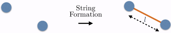
In the second case, one can consider a similar breaking chain but with a subtle difference, here the inflation occurs before the formation of monopole and string. The magnetic field of monopoles squeezes into flux tubes (CS) connecting pairs of monopoles and antimonopoles Lazarides et al. (1982); Vilenkin (1985). The strings gradually shrink and lead to the annihilation of monopole and antimonopole pairs. Fig. 12, shows an example of a chain where this gastronomy scenario occurs is $3221\to 3211\to 321$ . While $3221\to 3211$ results in the production of monopoles, the second breaking $3211\to 321$ connects the monopoles to strings.

In a system where a string is attached to a pre-existing monopole Lazarides et al. (1982); Holman et al. (1992); Martin and Vilenkin (1996); Vilenkin and Shellard (2000), the monopole’s initial abundance is considered to be one per horizon at the formation as computed by Kibble Kibble (1976) and as a result, there is no GW amplitude. In a recent work Dunsky et al. (2022), it was shown that if the Kibble-Zurek mechanism Zurek (1985) is considered and the monopole-antimonopole freeze-out occurring in between monopole and string formation is taken into account, the monopole-antimonopole pairs annihilate in less than a Hubble time with a non-relativistic velocity. This situation again does not generate any GWs. On the other hand, if some of the monopoles with mass $m$ and string scale $v_{\mu}$ exist, then the monopole-bounded strings can be relativistic. They can generate GWs before decaying if the friction is not large.

Following the Kibble–Zurek mechanism, once formed, the monopole-antimonopole pairs start annihilating. Their freeze-out abundance at any temperature depends on the critical temperature $T_{c}$ ,Preskill (1979)

\displaystyle\frac{n_{m}(T)}{T^{3}}=\left[\frac{T_{c}^{3}}{n_{m}(T_{c})}+\frac{h^{2}}{\beta_{m}}\frac{CM_{Pl}}{m}\left(\frac{m}{T}-\frac{m}{T_{c}}\right)\right]^{-1}

(192)

With $n_{m}$ being the number density of monopoles, $C=(8\pi^{3}g_{*}/90)^{-1/2}$ , critical temperature $T_{c}$ corresponds to a temperature at which the vacua have degenerate energy and

\displaystyle\beta_{m}\simeq\frac{2\pi}{9}\sum_{i}b_{i}\left(\frac{he_{i}}{4\pi}\right)^{2}\ln{\Lambda}

(193)

counts the particles of charge $e_{i}$ in the background plasma that the monopole scatters off. The magnetic coupling is $h=2\pi/e$ , where $e$ is the $U(1)$ gauge coupling constant, $\Lambda\sim{1/(g_{*}e^{4}/16\pi^{2})}$ is the ratio of maximum to minimum scattering angles of charged particles in the plasma, and $b_{i}=1/2$ for fermions and $1$ for bosons Vilenkin and Shellard (2000); Goldman et al. (1981). With $e\sim 0.3$ and a comparable number of electromagnetic degrees of freedom as in the Standard Model, $\beta_{m}\sim 20$ .

At a scale below $v_{\mu}$ , the magnetic fields of the monopoles squeeze into flux tubes. The string length here is set by the typical separation distance between monopoles,

\displaystyle l\approx\frac{1}{n_{m}(T=v_{\mu})^{1/3}}.

(194)

Eq. 194 is valid when the correlation length of the string Higgs field denoted by $\xi_{\mu}$ follows the condition $\xi_{\mu}\geq l$ Vilenkin and Shellard (2000). Since the string correlation length grows fast enough with time $\propto t^{5/4}$ Kibble (1976); Vilenkin and Shellard (2000), the string-bounded monopole becomes straightened out within roughly a Hubble time of string formation and ends up with a length close to Eq. 194. For $T_{c}=v_{m}\lesssim 10^{17}\,\rm GeV$ , $l$ is far below the horizon scale. Consequently, $l$ is not conformally stretched by Hubble expansion and only can decrease with time by energy losses from friction and gravitational waves.

Because the string rest mass is converted to monopole kinetic energy, the initial string length Eq. 194 determines whether or not the monopoles can potentially move relativistically. Relativistic monopoles can emit a brief pulse of gravitational radiation before annihilating while non-relativistic monopoles will generally not. This can be achieved in a situation where $\beta\sim 1$ and $T^{2}\sim\mu$ (string tension) (see Dunsky et al. (2022) for details). Here, the pulse of energy density emitted by relativistic monopoles in the form of gravitational waves is well approximated by the product of the power emitted ( $P_{\rm GW}=\Gamma G\mu^{2}$ ) by oscillating monopoles connected to strings, the number density ( $n_{m}(v_{\mu})$ ) of monopoles at $T=v_{\mu}$ and the lifetime of the string-bounded monopoles $\tau$ ,

\displaystyle\rho_{\rm GW,burst}\approx n_{m}(v_{\mu})P_{\rm GW}\,\tau.

(195)

The GW amplitude from the burst is simply given by Eq. 195 and redshifted to the spectrum we see today,

	$\displaystyle\Omega_{\rm GW,burst}$	$\displaystyle=\frac{\rho_{\rm GW,burst}}{\rho_{c}(v_{\mu})}\Omega_{r}\left(\frac{g_{0}}{g_{}(v_{\mu})}\right)^{\scalebox{1.01}{$\frac{1}{3}$}}$			(196)
		$\displaystyle\approx\frac{30\pi^{2}}{g_{*}(v_{\mu})\beta}\Gamma G\mu\left(\delta\frac{m}{M_{\rm Pl}}\right)^{\scalebox{1.01}{$\frac{2}{3}$}},$			(196)

where

\displaystyle\delta=\frac{1}{C\beta_{m}h^{2}}\left(\frac{4\pi}{h^{2}}\right)^{2}\text{Max}\left\{1,\,\frac{v_{\mu}}{m}\left(\frac{\beta_{m}h^{2}}{4\pi}\right)^{2}\right\}.

(197)

and $\rho_{c}(v_{\mu})$ is the critical energy density of the Universe at string formation, which is assumed to be in a radiation-dominated era. The amount of monopole-antimonopole annihilation that occurs before string formation at $T=v_{\mu}$ is characterized by the argument of the ‘Max’ function of Eq. 197. For a small $v_{\mu}/m$ , the freeze-out annihilating monopoles finishes before string formation, and the max function of Eq. 197 saturates at $1$ . In this situation, $\delta\approx 10^{-4}\beta_{m}^{-1}(e/0.5)^{4}$ .

Similarly, the peak frequency for the burst is controlled by the inverse length which in turn is controlled by the symmetry-breaking scale,

\displaystyle f_{\rm burst}\sim\frac{1}{l}\frac{a(t_{\mu})}{a(t_{0})}

\displaystyle\approx 10^{8}\,{\rm Hz}\left(\frac{v_{m}}{10^{14}\,\rm GeV}\,\frac{\delta}{10^{-4}}\,\frac{106.75}{g_{*}(v_{\mu})}\right)^{\scalebox{1.01}{$\frac{1}{3}$}}

(198)

where $a(v_{\mu})$ and $a(t_{0})$ are the scale factors at string formation and today, respectively.

With the understanding of the monopole burst spectrum, one can compute $\Omega_{\rm GW}$ for a situation where $\beta_{m}\sim 1$ . Applying the chain rule, one can replace $\frac{dn(l,t^{\prime})}{dl}$ in Eq.189 with

\frac{dn}{dl}(l,t^{\prime})=\frac{dn}{dt_{k}}\frac{dt_{k}}{dl}.

(199)

where primed coordinates refer to the time of emission and unprimed refer to the present so that gravitational waves emitted from the monopoles at time $t^{\prime}$ with frequency $f^{\prime}$ will be observed today with frequency $f=f^{\prime}a(t^{\prime})/a(t)$ . Further, $t_{k}$ is the formation time of monopole-bounded strings of length $l(t_{k})$ ,

\displaystyle\frac{dn}{dt_{k}}\simeq n_{m}(t_{k})\delta(t_{k}-t_{\mu})\left(\frac{a(t_{k})}{a(t)}\right)^{3}

(200)

is the string-bounded monopole production rate, which is localized in time to the string formation time, $t_{\mu}\simeq CM_{Pl}/v_{\mu}^{2}$ . $dt_{k}/dl$ is found by noting that the energy lost by relativistic monopoles separated by a string of length $l$ which is given by by the rate of change in string length and monopole mass,

\displaystyle\frac{dE}{dt}=\frac{d}{dt}(\mu l+2m)\approx-\beta_{m}v^{2}\mu\,.

(201)

A relativistic monopole can be achieved when $\mu l\gg 2m$ Dunsky et al. (2022). As a result, monopole-bounded strings that form at time $t_{k}$ with initial size $l(t_{k})$ decrease in length according to

\displaystyle l(t)\simeq l(t_{k})-\beta_{m}v^{2}(t-t_{k})

(202)

so that

\displaystyle\frac{dt_{k}}{dl}\simeq\frac{1}{\beta_{m}v^{2}}\approx 1.

(203)

The normalized power spectrum for a discrete spectrum can be decomposed into the product of the delta function and fractional power radiated by the $n^{th}$ mode of an oscillating string loop,

\displaystyle g(x)=\sum_{n}\mathcal{P}_{n}\delta(x-n\xi)\qquad\xi\equiv\frac{l}{T}

(204)

ensures the emission frequency of the $n$ th harmonic is $f^{\prime}=n/T$ , where $T$ is the oscillation period of the monopoles. For pure string loops, $T=l/2$ ( $\xi=2$ , reducing to Eq. 190), whereas for monopoles connected to strings, $T=2m/\mu+l\simeq l$ Leblond et al. (2009); Martin and Vilenkin (1997) ( $\xi\approx 1$ ). $\mathcal{P}_{n}\approx n^{-1}$ is found Leblond et al. (2009); Martin and Vilenkin (1997) for harmonics up to $n\approx\gamma_{0}^{2}$ , where $\gamma_{0}\simeq(1+\mu l/2m)$ , is the Lorentz factor of the monopoles. For $n>\gamma_{0}^{2}$ , $P_{n}\propto n^{-2}$ , $\Gamma\approx 4\ln\gamma_{0}^{2}$ .

In this situation, a string eats the monopole, and the emitted GW spectrum looks like,

\displaystyle\Omega_{\text{GW}}=\sum_{n}\frac{8\pi(G\mu)^{2}}{3H_{0}^{2}}\bigg{(}\frac{a(t_{\mu}-l_{*})}{a(t-0)}\bigg{)}^{5}\bigg{(}\frac{a(t_{\mu})}{a(t_{\mu}-l_{*})}\bigg{)}^{3}\times\Gamma\mathcal{P}_{n}\frac{\zeta n}{f}\frac{n_{m}(t_{\mu})}{\beta_{m}v^{2}}

(205)

where

\displaystyle l_{*}=\frac{\frac{\zeta_{n}n}{f}\frac{a(t_{\mu})}{a(t_{0})}-n_{m}(t_{\mu})^{-1/3}}{\beta_{m}v^{2}}

(206)

The GW spectrum for this scenario is shown in the right panel of Fig. 14. Here, at high frequencies, the spectral shape goes as $f^{-1}$ , prior to which a small plateau is observed where the spectrum goes as $\text{ln}f$ and at low frequencies decays as $f^{3}$ .

•

String-Wall network: Analogous to a string-monopole system, the hybrid defects associated with a string-wall network Dunsky et al. (2022); Maji et al. (2023); Lazarides et al. (2023); Gelmini et al. (2021b, 2023b, 2023a); Maji et al. (2023); Li et al. (2023c) can also be categorized as either the destruction of a domain wall network by the nucleation of string-bounded holes on the wall that expand and eat the wall, or the collapse and decay of a string-bounded wall network by walls that eat the strings. If a vacuum manifold $\mathcal{H}/\mathcal{K}$ is disconnected but $\mathcal{G}/\mathcal{K}$ is connected, DWs are formed at transition from $\mathcal{H}\to\mathcal{K}$ and $\Pi_{0}(\mathcal{H}/\mathcal{K})\neq\mathcal{I}$ . The DWs of this nature are topologically unstable as $\Pi_{0}(\mathcal{G}/\mathcal{K})=\mathcal{I}$ . This instability is caused by the nucleation of string-bounded holes on the wall that expand and destroy the wall completely. As a consequence of Schwinger nucleation, a wall (formed after inflation) gets bounded by a string (formed before inflation) if both defects are related to the same discrete symmetry. Here, the wall’s rest mass energy is transformed into the string’s kinetic energy leading to its rapid expansion. This rapid expansion causes the collapse of the string wall system and produces GWs in the process.

To understand this, one can solve the Boltzmann equation Dunsky et al. (2022) for the total energy density, $\rho_{\rm GW}$ in the gravitational wave background,

\displaystyle\frac{d\rho_{\rm GW}}{dt}+4H\rho_{\rm GW}=\mathcal{A}\mathcal{B}\frac{G\sigma^{2}}{t}\theta(t_{\Gamma}-t)-x\frac{d\rho_{\rm DW}}{dt}\theta(t-t_{\Gamma}).

(207)

While the first term on the RHS of Eq. 207 corresponds to the rate of energy density lost into GWs by DWs at time $t$ in the scaling regime and prior to the nucleation, the second term shows the energy transferred into GWs after string began nucleating and eating the wall with $x\in[0,1]$ denoting an efficiency parameter characterizing the fraction of the energy density of the wall transferred into gravitational waves at time,

\displaystyle t_{\Gamma}\sim\frac{1}{\sigma A}e^{S_{E}}\sim\frac{1}{\sigma^{1/3}}\exp{\frac{16\pi\kappa_{s}}{9}}.

(208)

Here, we take the wall area, $A$ at time $t_{\Gamma}$ to be $\sim t_{\Gamma}^{2}$ following the scaling regime and $\kappa_{s}=\mu^{3}/\sigma^{3}$ where $\sigma$ denotes the surface tension of the DW that depends on the breaking scale $v_{\sigma}$ that leads to the formation of the DW (see section IV.2 for details). Also one needs to have $\mu^{3}\sim\sigma^{3}$ , otherwise, the DW remains long-lived. When the strings begin nucleating at $t_{\Gamma}$ , they quickly expand from an initial radius $R_{\rm tp}=2R_{c}$ with $R_{c}\equiv\mu/\sigma$ according to Dunsky et al. (2022)

\displaystyle R_{s}(t)=\sqrt{4R_{c}^{2}+(t-t_{\Gamma})^{2}}.

(209)

In the above, $R_{\rm tp}$ denotes the critical string radius that is obtained when the balance between string creation and domain wall destruction is balanced. Above this, it is energetically favorable for the string to nucleate and continue expanding and consuming the wall as shown in the top panel of Fig. 16. As a result, the strings rapidly accelerate to near the speed of light as they ‘eat’ the wall. The increase in string kinetic energy arises from the devoured wall mass. Thus, shortly after $t_{\Gamma}$ , most of the energy density of the wall is transferred to strings and string kinetic energy.

Assuming a conservative limit $x=0$ Dunsky et al. (2022), the solution to Eq. 207 during an era with scale factor expansion $a(t)\propto t^{\nu}$ is then

\displaystyle\rho_{\rm GW}(t)

\displaystyle=\Bigg{\{}\begin{array}[]{cc}\mathcal{A}\mathcal{B}\frac{G\sigma^{2}}{4\nu}\left(1-\left(\frac{t_{\rm scl}}{t}\right)^{4\nu}\right)&\;t\leq t_{\Gamma}\\ \left(\rho_{\rm GW}(t_{\Gamma})+x\mathcal{A}\frac{\sigma}{{t_{\Gamma}}}\right)\left(\frac{a(t_{\Gamma})}{a(t)}\right)^{4}&\;t>t_{\Gamma}\end{array}

(212)

Eq. 212 demonstrates that the gravitational wave energy density background quickly asymptotes to a constant value after reaching scaling at time $t_{\rm scl}$ and to a maximum at the nucleation time $t_{\Gamma}$ . We thus expect a peak in the gravitational wave amplitude of approximately Dunsky et al. (2022),

\displaystyle\Omega_{\text{GW, max}}=\frac{16\pi}{3}[(G\sigma t_{\Gamma})^{2}+2xG\sigma t_{\Gamma}]\Omega_{r}\bigg{(}\frac{g_{*0}}{g_{*}(t_{\Gamma})}\bigg{)}^{1/3}.

(213)

where we take $t_{\Gamma}>t_{\rm scl}$ , $\mathcal{A}=\mathcal{B}=1$ , and a radiation dominated background at the time of decay with $\nu=\frac{1}{2}$ . $\Omega_{r}=9.038\times 10^{-5}$ is the critical energy in radiation today Aghanim et al. (2020b).

The first term in Eq. 213, the contribution to the peak amplitude from gravitational waves emitted prior to nucleation, agrees well with the numerical results of Hiramatsu et al. (2014) if $t_{\Gamma}$ maps to the decay time of unstable walls in the authors’ simulations. The second term in Eq. 213, the contribution to the peak amplitude from GW emitted after nucleation, has not been considered in numerical simulations. The post-nucleation contribution dominates the pre-nucleation contribution if $x\gtrsim G\sigma t_{\Gamma}$ , which may be important for short-lived walls. The complex dynamics of string collisions during the nucleation phase motivate further numerical simulations.

The frequency dependence on the gravitational wave amplitude may be extracted from numerical simulations of domain walls in the scaling regime. The form of the spectrum was found in Hiramatsu et al. (2014) to scale as

\displaystyle\Omega_{\text{GW}}(f)\simeq\Omega_{\text{GW, max}}\Bigg{\{}\begin{array}[]{cc}\left(\frac{f}{f_{p}}\right)^{-1}&f>f_{p}\\ \left(\frac{f}{f_{p}}\right)^{3}&f<f_{p}\end{array}

(216)

where

\displaystyle f_{\rm p}\sim\frac{1}{t_{\Gamma}}\frac{a(t_{\Gamma})}{a(t_{0})}

(217)

The infrared $f^{3}$ dependence for $f<f_{\rm p}$ arises from causality arguments for an instantly decaying source Caprini et al. (2009a). This behavior is shown in Fig. 17.

Finally, consider the case of a string wall network where DWs get attached to pre-existing strings Dunsky et al. (2022). Here, both strings and DWs are formed after inflation. In this scenario, the strings are formed before the wall formations and once the walls are in the picture they fill the spaces between the strings. After the DW-bounded string system enters the horizon, the system oscillates with constant amplitude resulting in the production of the GWs.

Considering a string boundary of a circular wall with radius $R$ , it was shown that while the wall tension dominates when the radius $R>>R_{c}$ with $R_{c}\equiv\mu/\sigma$ , the string dynamics reduces to the pure string loop motion for $R<<R_{c}$ where the string dominates the dynamics and the power is independent of loop size which is in agreement with the pure string case. Using the VOS model of an infinite string-wall network they showed that the walls pull their attached strings into the horizon when the curvature radius of the hybrid network grows above $R_{c}$ . Once this network is inside the horizon, it oscillates and radiates GWs. As expected, for $R<<R_{c}$ (pure string limit), the power emitted in the GWs goes as $P_{\rm GW}\propto G\mu^{2}$ . On the other hand, for $R>>R_{c}$ , the domain wall dominates the dynamics and the power deviates from the pure string case, increasing quadratically with $R/R_{c}$ . Since $R_{c}\equiv\mu/\sigma$ , this is equivalent to $P_{\rm GW}\propto G\sigma^{2}R^{2}\propto G\sigma M_{\rm DW}$ , in agreement with the quadrupole formula expectation for gravitational wave emission from domain walls.

With the idea of GW power emitted by a string-bounded domain wall system (see Dunsky et al. (2022) for detail) one can now calculate the gravitational wave spectrum from a network of circular string-bounded walls. Here we briefly discuss the analytical estimate of the expected amplitude and frequency of the spectrum. For the numerical computation, we refer readers to Dunsky et al. (2022).

To start with, first consider a pure string loop without walls that form at time $t_{k}$ with initial length $l_{k}=\alpha t_{k}$ , where $\alpha\simeq 0.1$ . Once these loops are inside the horizon, they oscillate, and their energy density redshifts $\propto a^{-3}$ because their energy $E=\mu l$ is constant in the flat space limit. The loops radiate GW with power $P_{\rm GW}=\Gamma_{s}G\mu^{2}$ as discussed above, where $\Gamma_{s}\approx 50$ , and eventually decay from gravitational radiation at time

\displaystyle t_{\Gamma}\approx\frac{\mu l_{k}}{\Gamma_{s}G\mu^{2}}\quad(\text{Pure string loop lifetime}).

(218)

When the pure string loops form and decay in a radiation-dominated era, their energy density at decay is

\displaystyle\rho(t_{\Gamma})\approx\mu l_{k}n(t_{k})\left(\frac{t_{k}}{t_{\Gamma}}\right)^{3/2}

(219)

with $n(t_{k})\approx\frac{1}{3}\frac{\mathcal{F}C_{\rm eff}}{\alpha t_{k}^{3}}$ being the initial number density of loops of size $l_{k}$ that break off from the infinite string network in a scaling regime Cui et al. (2019); Gouttenoire et al. (2020); Sousa and Avelino (2013b), $\mathcal{F}\approx 0.1$ Blanco-Pillado et al. (2014) and $C_{\rm eff}\approx 5.4$ in a radiation dominated era Cui et al. (2018); Blasi et al. (2020). Following Eq. 218 and Eq. 219, the gravitational wave amplitude coming from these pure string loops is approximately

	$\displaystyle\Omega_{\rm GW}^{(\rm str)}$	$\displaystyle\approx$	$\displaystyle\frac{\rho(t_{\Gamma})}{\rho_{c}(t_{\Gamma})}\Omega_{\rm r}\left(\frac{g_{0}}{g_{}(t_{\Gamma})}\right)^{\scalebox{1.01}{$\frac{1}{3}$}}$
		$\displaystyle=$	$\displaystyle\frac{32\pi}{9}\mathcal{F}C_{\rm eff}\sqrt{\frac{\alpha G\mu}{\Gamma_{s}}}\Omega_{\rm r}\left(\frac{g_{0}}{g_{}(t_{\Gamma})}\right)^{\scalebox{1.01}{$\frac{1}{3}$}}$

where $\rho_{c}(t_{\Gamma})$ is the critical energy density of the Universe at $t_{\Gamma}$ .

Before reaching $t=t_{*}$ , the dynamics of the string-bounded walls are dominated by the strings and the spectrum must be approximately that of a pure string spectrum with $\Omega_{\rm GW}$ given approximately by Eq. • ‣ IV.5, independent of frequency. Now at time $t_{k}=t_{*}$ , let us consider the formation of a near circular string-bounded wall with initial circumference $l_{k}=\alpha t_{k}$ . While for $l_{k}\lesssim 2\pi R_{c}$ , the power emitted and total mass of the system is effectively identical to the pure string case and $\Omega_{\rm GW}$ remains the same as Eq. • ‣ IV.5, for $l_{k}\gtrsim 2\pi R_{c}$ , the power emitted and mass of the system is dominated by the DW contribution of the wall-string piece. In this situation, the wall-bounded string decays while radiating the GW at the time

\displaystyle t_{\Gamma}\approx\frac{\sigma l_{k}^{2}/4\pi}{\Gamma(l_{k})G\mu^{2}}\approx\frac{1}{G\sigma}

(221)

For the wall-bounded strings forming and decaying in a radiation-dominated era, their energy density at decay is

\displaystyle\rho(t_{\Gamma})\approx\frac{\sigma l_{k}^{2}}{4\pi}n(t_{k})\left(\frac{t_{k}}{t_{\Gamma}}\right)^{3/2}

(222)

where $n(t_{k})\approx\frac{1}{3}\frac{\mathcal{F}C_{\rm eff}}{\alpha t_{k}^{3}}$ follows from the infinite string-wall network being in the scaling regime with $\mathcal{F}$ and $C_{\rm eff}$ expected to be similar to the pure string values right before the infinite network collapses at $t_{*}$ . Hence the GW amplitude in this scenario is controlled by the energy density of the string-wall system at decay,

	$\displaystyle\Omega_{\rm GW}$	$\displaystyle\approx$	$\displaystyle\frac{\rho(t_{\Gamma})}{\rho_{c}(t_{\Gamma})}\Omega_{r}\left(\frac{g_{0}}{g_{}(t_{\Gamma})}\right)^{1/3}$
		$\displaystyle=$	$\displaystyle\frac{8}{9}\mathcal{F}C_{\rm eff}\alpha\sqrt{G\sigma t_{k}}\Omega_{r}\Big{(}\frac{g_{0}}{g_{}(t_{\Gamma})}\Big{)}^{\scalebox{1.01}{$\frac{1}{3}$}}\,.$

The largest amplitude of Eq. • ‣ IV.5 occurs at the latest formation time $t_{k}$ , which is $t_{*}$ , the time of the collapse of the infinite network. As a result of this, a ‘bump’ relative to the flat string amplitude appears if

\displaystyle\frac{\Omega_{\rm GW}}{\Omega_{\rm GW}^{(\rm str)}}\approx\frac{1}{4\pi}\sqrt{\frac{\Gamma_{s}\alpha t_{*}}{R_{c}}}\approx 0.2\left(\frac{\alpha}{0.1}\right)^{\scalebox{1.01}{$\frac{1}{2}$}}\left(\frac{\Gamma_{s}}{50}\right)^{\scalebox{1.01}{$\frac{1}{2}$}}\left(\frac{t_{*}}{R_{c}}\right)^{\scalebox{1.01}{$\frac{1}{2}$}}

(224)

is greater than $1$ and at a frequency

\displaystyle f_{\rm peak}\sim\frac{1}{l_{k}}\frac{a(t_{\Gamma})}{a(t_{0})}.

(225)

since the walls remain the same size once inside the horizon and dominantly emit at the frequency of the harmonic, $f_{\rm emit}\sim l_{k}^{-1}$ . Here, $l_{k}\approx\alpha t_{*}$ .

The estimation of Eq. 224 indicates that if $t_{*}>>R_{c}$ , then $\Omega_{\rm GW}$ features a ‘bump’ relative to the flat string spectrum before decaying. In this situation, the walls are massive and large enough to live much longer than the pure string of the same size. Due to this, they have an enhanced energy density before decaying in comparison to the shorter-lived pure string loops. In a situation with $t_{*}\approx R_{c}$ no such enhancement is observed because string-bounded walls are smaller in size and decay quickly.

With the qualitative features of the spectrum understood, we turn to a numerical computation of $\Omega_{\rm GW}$ . The GW spectrum obtained from the numerical computation of Dunsky et al. (2022) for this system is shown in the right panel of Fig. 17 for a fixed value of $\sqrt{\mu}=10^{12}$ GeV. It is also interesting to point out that, the spectrum here decays as $f^{3}$ (due to causality) rather than $f^{2}$ decay signal which was observed in the situation with the monopoles eating the strings.

IV.6 Applications of gravitational waves from topological defects

Cosmic strings as discussed earlier, can play a vital role in understanding and testing the evolutionary history of the Universe. A string network continuously emits gravitational wave power for the entirety of its existence, and as the string network enters the scaling regime, the fraction of energy density in gravitational waves should remain constant for all frequencies unless there is some change in the energy budget of the Universe. GW signals emitted from the CS can therefore provide an unprecedented window into the evolution of the very early universe before BBN and the CMB. On the other hand, if a network of CS that was formed before or shortly after the start of inflation can regrow after getting diluted and generate GW signals that can be observed today. In this section, we will first cover how strings can be witnesses to a period of inflation before covering how they can be witnesses to dramatic changes in the Universe such as an early period of matter domination or kination. Finally, we will cover how topological defects can provide information about high-scale physics from leptogenesis to quantum gravity.

As is well known, primordial cosmological inflation dilutes all the relics that were generated before its commencement to a negligible level, hence one expects that a CS if produced before the onset of inflation will also be diluted. A recent study Cui et al. (2020), has shown that a network of cosmic strings diluted by inflation can replenish to a level that can result in the generation of GW signals that can be probed by the present and future GW detectors. This is due to the energy density diluting slower than radiation. Unlike the signals that result from an undiluted CS which are of the form of SGWB, the signal resulting from the diluted CS can be distinctive bursts of GWs.

To understand this, we assume a constant Hubble parameter $H_{I}=V_{I}/3M_{\text{Pl}}^{2}$ during inflation that describes the inflationary energy density from the initial time $t_{I}$ to end time $t_{E}$ with $V_{I}=M^{4}$ ( $M\leq 10^{16}$ GeV Akrami et al. (2020b)), the cosmological scale factor grows as $a(t)\propto e^{H_{I}t}$ . Once the inflation is completed, the radiation-dominated era is initiated with temperature $T_{RH}\leq(30/\pi^{2}g_{*})^{1/4}M$ . Under the assumption that the temperature during the reheating remains below the symmetry breaking scale, the dilution of the pre-existing CS by thermal processes like symmetry restoration can be avoided. Once again following the VOS model used for describing the horizon-length long strings during and after inflation Guedes et al. (2018), one can study the evolution of the correlation length parameter $L$ and the velocity parameter $\bar{v}$ of a long string Martins and Shellard (1996, 2002). Starting with the initial conditions,

L(t_{F})\equiv L_{F}=\frac{1}{\xi H_{I}},

(226)

where $\xi^{2}$ corresponds approximately to the number of long strings within the Hubble volume at time $t_{F}$ . $L(t)$ soon reaches an attractor solution during inflation after $t_{F}$ ,

L(t)=L_{F}e^{H_{I}(t-t_{F})},~{}\bar{v}(t)=\frac{2\sqrt{2}}{\pi}\frac{1}{H_{I}L(t)}.

(227)

For $HL>>1$ and $\bar{v}<<1$ , the above solution corresponds to the dilution of the long string network. As a result of this, the evolution of the string network after inflation takes a very simple form while $HL>>1$ with $(L/a)$ approximately constant. It follows that $HL$ decreases after inflation, corresponding to the gradual regrowth of the string network. If the network is to produce a potentially observable signal in GWs, at least a few strings are needed within our current Hubble volume corresponding to $HL\leq 1$ today. The conditions under which there is enough string regrowth for $HL\to 1$ while also maintaining a sufficient amount of inflation can be obtained by comparing the evolution of $L$ before scaling to that of the curvature radius $R=1/(H\sqrt{|\Omega-1|})$ which evolves in precisely the same way, independently of the details of inflation or reheating. The total number of inflationary e-foldings can then be written as $N_{tot}=H_{I}(t_{E}-t_{I})\equiv N_{F}+\Delta N$ with $\Delta N\geq 0$ being the number of e-foldings between $t_{I}$ and $t_{F}$ . Note that $\Delta N=0$ corresponds to the string forming before or at the start of inflation. Applying the curvature limit $|\Omega_{0}-1|=0.0007\pm 0.0037$ Aghanim et al. (2020b), one finds,

\Delta N+\ln\xi\geq 2.7+\frac{1}{2}\ln(|\Omega_{I}-1|)+\frac{1}{2}\ln\left[\Omega_{\Lambda}(1+\tilde{z})^{-2}+\Omega_{m}(1+\tilde{z})+\Omega_{r}(1+\tilde{z})^{2}\right]

(228)

where $\tilde{z}$ is the redshift at which $HL\to 1$ , $\Omega_{a}$ are the fractional energy densities in dark energy, matter, and radiation relative to critical today, $|\Omega_{I}-1|$ is the deviation from flatness at the start of inflation, $\ln(|\Omega_{0}-1|)/2\leq 2.7$ is the bound from Planck Aghanim et al. (2020b), and the last line describes the additional evolution of $(\Omega-1)$ between $\tilde{z}$ and now.

As discussed previously, the scaling solution produces larger string loops together with the smaller loops. The smaller loops are highly relativistic and most of the energy transferred to the smaller loops is in the form of kinetic energy that simply redshifts away, and thus larger loops are expected to be the dominant source of GWs. For a Nambu-Goto string large loops oscillate, emit energy in the form of GWs, and gradually shorten as shown in Eq. 174. Unlike the vanilla case discussed in section IV.3, the GW in this situation is mostly emitted by short, violent, collimated bursts involving cusps or kinks on the string loops. Bursts emitted by a cosmic string network over its cosmic history that are not resolved contribute to the characteristic stochastic gravitational wave background of the network. For comparing the GW signals with current and future detectors, one can separate the contributions of the recent burst (with large amplitude) and earlier bursts (unresolved). Recent bursts can also be potentially observed as distinct, individual events. If a burst is to be resolved in a given frequency band $f$ , it must produce a strain greater than the experimental sensitivity $h>h_{\rm exp}$ with a rate less than $f$ . The rate of such events is Siemens et al. (2006); Auclair et al. (2020); Cui et al. (2020)

\displaystyle R_{\rm exp}(f)=\int_{0}^{z_{*}}\!dz\int_{\max(h_{\rm min},h_{\rm exp})}^{h_{\rm max}}\!\!\!dh\;\frac{d^{2}R}{dz\,dh}(h,z,f)~{}~{}~{}~{}~{}\

(229)

where $z_{*}$ (denotes the largest redshift contributing to the rate) enforces the rate condition and is given by

\displaystyle f=\int_{0}^{z_{*}}\!dz\int_{h_{\rm min}}^{h_{\rm max}}\!dh\;\frac{d^{2}R}{dz\,dh}(h,z,f)\,.

(230)

Unresolved bursts contribute to the SGWB as Siemens et al. (2006); Auclair et al. (2020)

\displaystyle\Omega_{\rm GW}(f)=\frac{4\pi^{2}f^{3}}{3H_{0}^{2}}\int_{z_{*}}^{\infty}\!dz\,\int_{h_{\rm min}}^{h_{\rm max}}\!dh\;h^{2}\,\frac{d^{2}R}{dz\,dh}(h,z,f)

(231)

with $\Omega_{GW}=(f/\rho_{c})\,d\rho_{\rm GW}/df$ and

\displaystyle\frac{d^{2}R}{dz\,dh}

\displaystyle=

\displaystyle\frac{2^{3(q-1)}\,\pi\,G\mu\,N_{q}}{(2-q)}\frac{r(z)}{(1+z)^{5}H(z)}\,\frac{n(l,z)}{h^{2}f^{2}}

(232)

where $l$ is a function of $h$ , $f$ , and $z$ , and

\displaystyle h_{\rm min}=\frac{1}{(1+z)f^{2}}\frac{G\mu}{r(z)}\ ,~{}h_{\rm max}=\frac{[\alpha L(z)]^{q-2}}{f^{q}(1+z)^{q-1}}\frac{\,G\mu}{r(z)}

(233)

Since the total GW signal is expected to be dominated by bursts from cusps Ringeval and Suyama (2017); Blanco-Pillado and Olum (2017), one can set $q=4/3$ and $N_{q}=2.13$ (to match $\Gamma=50$ Auclair et al. (2020)) for the analysis purpose.

The top (bottom) panel of Fig. 18 shows the variation of the SGWB spectrum obtained from the unresolved (resolved) burst rate with frequency for diluted and undiluted string networks. The SGWB for the diluted networks falls off as $f^{-1/3}$ at high frequency due to the inclusion of the sufficient number of modes when computing the SGWB with the normal mode method (see Cui et al. (2020)) for the details. At higher frequencies, a sharper drop is observed from the burst method that results from the subtraction of infrequent bursts from the SGWB.

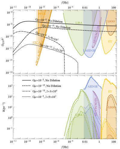
Let us now turn our attention to how the GW emitted from the CS can help us understand the cosmic history of the Universe after the inflation but at times well before primordial nucleosynthesis and the cosmic microwave background where standard cosmology has yet to be tested. Recent studies like Cui et al. (2018, 2019), have demonstrated how the spectrum of GWs emitted by a Nambu-Goto cosmic string network depends on the energy content of the universe when they are produced. For example, if the Universe transitions from radiation domination at very high temperatures to matter domination and then back to radiation domination before the onset of BBN, a GW spectrum can be observed that is different from what is seen in the standard cosmology and hence can be distinguished.

In a scenario like this, one can use the cosmological time $t_{\Delta}$ (epoch of most recent radiation-domination era) to calculate the frequency $f_{\Delta}$ where such a deviation would appear. The first significant modification in the frequency spectrum will appear when the dominant emission time $\tilde{t}_{M}$ comes from loops created at $t_{i}^{(k=1)}\simeq t_{\Delta}$ . This results in an approximate transition frequency $f_{\Delta}$ as the solution of

\displaystyle t_{i}(\tilde{t}_{M}(f_{\Delta}))=t_{\Delta}\ .

(234)

Under the approximation $a(t)\propto t^{1/2}$ at the radiation dominated era one can obtain Cui et al. (2018, 2019)

	$\displaystyle f_{\Delta}$	$\displaystyle\simeq$	$\displaystyle\sqrt{\frac{8\,z_{\rm eq}}{\alpha\,\Gamma G\mu}}\,\bigg{(}\frac{t_{eq}}{t_{\Delta}}\bigg{)}^{1/2}\,t_{0}^{-1}$
		$\displaystyle\simeq$	$\displaystyle\sqrt{\frac{8\,}{z_{\rm eq}\alpha\,\Gamma G\mu}}\,\bigg{[}\frac{g_{}(T_{\Delta})}{g_{}(T_{0})}\bigg{]}^{1/4}\bigg{(}\frac{T_{\Delta}}{T_{0}}\bigg{)}\,t_{0}^{-1}$

where $z_{\rm eq}\simeq 3387$ is the redshift at matter-radiation equality, and $T_{0}=2.725\,\text{K}$ is the temperature today. A more accurate dependence is obtained by fitting it to a full numerical the calculation that properly accounts for variations in $g_{*}$ gives Cui et al. (2018, 2019)

\displaystyle f_{\Delta}=(8.67\times 10^{-3}\,{\rm Hz})\,\bigg{(}\frac{T_{\Delta}}{\text{Gev}}\bigg{)}\bigg{(}\frac{0.1\times 50\times 10^{-11}}{\alpha\,\Gamma\,G\mu}\bigg{)}^{1/2}\left(\frac{g_{*}(T_{\Delta})}{g_{*}(T_{0})}\right)^{\frac{8}{6}}\left(\frac{g_{*S}(T_{0})}{g_{*S}(T_{\Delta})}\right)^{-\frac{7}{6}}\ .

(236)

This is found to be accurate to about $10\%$ . One can reinterpret this $f_{\Delta}$ as a frequency required to test cosmology up to temperature $T_{\Delta}$ . This is because the measured GW spectrum obtained from the CS will remain approximately flat till $f_{\Delta}$ for a given value of $\alpha$ and $\Gamma G\mu$ and hence would provide strong evidence for radiation domination up to the corresponding temperature $T_{\Delta}$ .

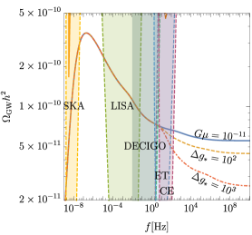
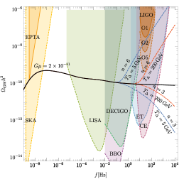
Such cosmological modification can be observed in a scenario having a very large number of additional degrees of freedom present in the spectrum at high energy. If additional degrees of freedom exist till temperature $T_{\Delta}$ , the energy density of GW will be altered above $f_{\Delta}$ in comparison to what is expected in a standard cosmology with only SM degrees of freedom. In such a scenario, one obtains a standard $\Omega_{\rm GW}(f)$ vs. $f$ for cosmic strings behaviour up to $f_{\Delta}$ and thereafter fall-off is observed for $f>f_{\Delta}$ as shown in left panel of Fig. 19. For a detailed discussion see Cui et al. (2018, 2019).

The refs. Cui et al. (2018, 2019) also discuss scenarios where GWs from cosmic strings evolve in a non-standard phase, either of an early matter domination phase $(n=3)$ or an early kination $(n=6)$ phase where $\rho\propto a^{-n}$ denotes the dilution of energy density of different dominant phases. The early matter domination can result from the presence of a new degree of freedom whose late decay brings the Universe back to the radiation domination era. Such slow decay should also satisfy BBN constraints. In other words, the universe transitions from radiation domination at very high temperatures to matter domination and then back to radiation domination (by the decay of said particles) before the onset of BBN. Another captivating way to generate such deviation is to consider a scalar $\phi$ oscillating into a potential of form $V(\phi)\propto\phi^{N}$ that gives $\rho\propto a^{-6N/(N+2)}$ . In the limit $N\to\infty$ one finds a phase with $n=6$ , the scalar can then decay. This leads to a cosmological history of very early radiation domination to kination domination (oscillation energy dominating) and back to radiation (by the decay of the moduli). CS can act as a tool to probe these scenarios of alternate cosmologies, this is because they rapidly enter a scaling regime $i.e.$ their energy density scales with scale factor $a$ the same as the dominant energy density of the Universe. While for an early matter domination era, the CS will scale like $a^{3}$ during that phase, an early kination phase will make cosmic strings scale as $a^{6}$ . The modified scaling behavior of CS will alter the energy density of the GWs emitted through its non-standard redshifting. Cui et al. (2018, 2019) shows these effects quantitatively, which leads to a sharp fall-off in $\Omega_{\rm GW}(f)$ at high frequency $f$ (corresponding to the new phase era) if there is early matter domination and a sharp rise in $\Omega_{\rm GW}(f)$ if there is an early kination phase. This is shown in the right panel of Fig. 19

Apart from testing the scenarios of modified cosmologies, a GW emitted from the CS can also help in testing the other early Universe physics like why there exists a plethora of matter over anti-matter in our Universe. Arguably the most elegant way to understand this issue is through leptogenesis Fukugita and Yanagida (1986); Luty (1992); Pilaftsis (1997), using type I seesaw mechanism Minkowski (1977); Yanagida (1979a, b); Gell-Mann et al. (1979); Mohapatra and Senjanovic (1980); Schechter and Valle (1980, 1982); Datta et al. (2021); Dutta Banik et al. (2021); Datta et al. (2021); Bhattacharya et al. (2021, 2023b)¹⁴¹⁴14A recent work King et al. (2023a) has also shown a new method towards distinguishing the Dirac vs Majorana nature of neutrino masses from the spectrum of GW associated with the neutrino mass genesis.. Here an out-of-equilibrium decay of a heavy state generates an asymmetry in between leptons and their antiparticles. Once generated, the lepton asymmetry catalyzes a baryon asymmetry through sphaleron transitions Kuzmin et al. (1985); Bento (2003); D’Onofrio et al. (2014). Unfortunately, the scale of leptogenesis is much beyond the scales that can be tested on present-day earth-based detectors. The mass of the Right-handed neutrinos (RHN) responsible for explaining the light neutrino masses lies below the Planck or a possible GUT scale suggesting some symmetry that survives below these scales to protect the right-handed neutrino mass. Thermal leptogenesis demands the breaking of this symmetry to be below the scale of inflation or the asymmetry will be catastrophically diluted. Such a breaking can be observed through its predicted cosmological defects. In Dror et al. (2020), a $B-L$ that protects the RHN masses is spontaneously broken to generate the RHN masses, this process also results in the generation of CS that radiates a spectrum of stochastic gravitational waves. When embedding this symmetry into a grand unified group, one finds that the majority of viable symmetry-breaking paths admit cosmic strings. The GW signal is expected to be tested using future detectors that are expected to probe the entire mass range relevant to the paradigm of thermal leptogenesis.¹⁵¹⁵15If it is a global symmetry protecting the seesaw mass, it is still possible a signal is visible if the seesaw scale is very high Fu et al. (2023a) Symmetry breaking paths that do not admit cosmic strings could result in a signal from proton decay King et al. (2021b, a); Saad (2023); Fu et al. (2023b). Recent work has also considered the complementarity of gravitational waves and neutrino oscillation experiments within the concrete framework of an SO(10) model Fu et al. (2022). A diagrammatic representation of the breaking chains of $SO(10)\to G_{\rm SM}$ is shown in Fig. 20 .

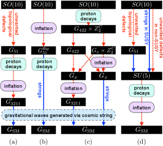
Like CS, the GW resulting from the DW can also play an interesting role in understanding the physics of the early Universe King et al. (2023c, b); Barman et al. (2023b). For example, recent works like King et al. (2023c, b), have explored the phenomenological consequences of breaking discrete global symmetries in quantum gravity (QG) ¹⁶¹⁶16On the other hand Barman et al. (2023b) discusses the possibility of detecting the scale of Dirac leptogenesis through GW generated from DW annihilation.. Motivated by Swampland global symmetry conjecture Banks and Dixon (1988); Banks and Seiberg (2011); Harlow and Shaghoulian (2021) which says that there exists no exact global symmetry in effective field theories (EFTs) arising from UV theories of QG, they studied how quantum gravity effects, manifested through the breaking of discrete symmetry responsible for both Dark Matter and Domain Walls, can have observational effects through CMB observations and gravitational waves. They show that the existence of very small bias terms stems from the QG ¹⁷¹⁷17Work like Lu and Chiang (2023) showed that a small bias can also be achieved in a clockwork axion model where the QCD axion potential induced by the QCD phase transition can serve as an energy bias leading to the annihilation of DW which allows DWs to annihilate, thus stopping them from dominating the energy density of the Universe. To illustrate this idea, in King et al. (2023c), they considered a simple model with two singlet scalar fields together with two $Z_{2}$ symmetries, one being responsible for DM stability, and the other spontaneously broken and responsible for DWs.¹⁸¹⁸18For the fermionic DM see King et al. (2023b). Explicit due to QG causes the DM to be allowed to mix with the SM neutrinos after the electroweak symmetry breaking. This causes the DM to become unstable. Such DM decay puts constraints on the QG operator from the CMB, BBN, galactic and extragalactic diffuse $X/\gamma$ -ray background, SKA, neutrinoless double beta decay. Moreover, both the $Z_{2}$ symmetries are assumed to be explicitly broken by QG effects by operators at the same mass dimension and with the same effective Planck scale. They showed that this hypothesis led to observable GW signatures from the annihilation of DWs, which are correlated with the decaying DM signatures constrained by CMB observations.¹⁹¹⁹19This is also a possible explanation for the results of the NANOGrav Agazie et al. (2023a); Afzal et al. (2023b), the EPTA Antoniadis et al. (2023b, c), the PPTA Reardon et al. (2023) and the CPTA Xu et al. (2023) Fig. 21 shows constraints obtained on the QG scale.

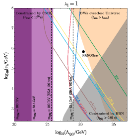
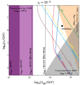
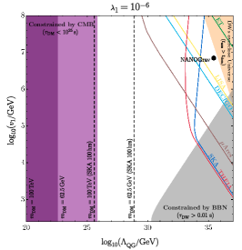
GW detectors have given us a window to early universe cosmology complementary to any other probes previously developed. A strong and well-understood source of GWs in the early universe could give us unprecedented ability to probe cosmological energy evolution of the early universe far earlier than previously attainable. These works have also demonstrated that topological defects if they exist, would be excellent standard candles to achieve these aims.

V Scalar induced gravitational waves

It was first mentioned by Tomita Tomita (1967) then rediscovered by Matarrese, Pantano, and Saez Matarrese et al. (1993, 1994) that large scalar perturbations can act as a source for tensor perturbations at second order. For a curvature perturbation power spectrum, ${\cal P}_{\cal R}$ , the approximate scaling of scalar induced gravitational waves are²⁰²⁰20In this review we focus on gravitational waves induced by curvature perturbations generated by ultra slow roll or by sudden changes in the equation of state. It is also possible to induce gravitational waves from isocurvature perturbations Domènech et al. (2022); Bhaumik et al. (2022); Lozanov et al. (2023), or through spectator fields during inflation Biagetti et al. (2013). For a review see Domènech (2023)

\Omega_{\rm GW}^{\rm induced}h^{2}\sim\frac{1}{12}\Omega_{r,0}h^{2}{\cal P}^{2}_{\cal R}\sim 10^{-6}{\cal P}^{2}_{\cal R}.

(237)

In vanilla cosmology, the scalar power spectrum after inflation can be inferred from CMB extrapolation ${\cal P}_{\cal R}\sim 10^{-9}$ Akrami et al. (2020a) which means that absent any enhancement, $\Omega_{\rm GW}^{\rm induced}h^{2}\sim 10^{-24}$ , which is far too small for any detector in the foreseeable future. The enhancement can occur during a period of ultra-slow roll inflation, a large change in the field angle in multifield inflation, or due to the evolution of scalar perturbations after inflation Domènech (2021). For example, a sudden change in the equation of state can dramatically enhance the gravitational wave spectrum Hooshyar (2009); Alabidi et al. (2013); Inomata et al. (2019b, a). Scalar-induced gravitational waves have a remarkable range of applications. For instance, if there exists an instability scale as hinted at in the Standard Model Altarelli and Isidori (1994); Casas et al. (1996); Hambye and Riesselmann (1997); Sher (1989); Arnold (1989); Isidori et al. (2001); Ellis et al. (2009); Elias-Miro et al. (2012); Degrassi et al. (2012); Bezrukov et al. (2012); Bednyakov et al. (2015); Buttazzo et al. (2013); Espinosa et al. (2017), there should be a scalar induced gravitational wave spectrum Espinosa et al. (2018c). As the running of the Higgs quartic self-interaction could be affected by any number of hypothetical particles in the mass range between the weak scale and the instability scale, gravitational wave detectors may be the only way to tell if the electroweak vacuum is stable. Further, if the Baryon asymmetry was produced during the Affleck Dine mechanism, there was likely a period of Q-ball domination whose sudden decay results in a gravitational wave spectrum, one of the few ways to test this paradigm White et al. (2021). Finally, if one produces primordial Black holes that are too small to survive after Big Bang nucleosynthesis before evaporating via Hawking radiation, these black holes can dominate the Universe and their decay rate is again surface-to-volume suppressed which results in a sudden transition from matter to radiation Inomata et al. (2020). We summarize the range of applications in section V.5 in slightly more depth. For now, we emphasize the extraordinary promise of this source of gravitational waves.

In this section, we review the current formalism and our understanding of both causes of scalar-induced gravitational waves and present some recent applications.

V.1 Enhanced scalar power spectrum during inflation

When large scalar perturbations reenter the horizon after inflation they can produce a detectable source of gravitational waves Garcia-Bellido and Ruiz Morales (2017); Ezquiaga et al. (2018); Ballesteros and Taoso (2018); Li et al. (2023a, b); Wang et al. (2023b); Zhao et al. (2023b); Yu and Wang (2023) (for a review, see Domènech (2021)). Consider the slow roll parameters for a scalar field in an expanding background

\epsilon=-\frac{\dot{H}}{H}\ ,\epsilon_{2}=\frac{2\ddot{\phi}}{H\dot{\phi}}+2\epsilon\ .

(238)

The slow roll conditions are of course that the above parameters are small. However, near an inflection point when $V^{\prime}\to 0$ , the Klein Gordon equation in an expanding background yields $\ddot{\phi}=-3H\dot{\phi}$ and we have

\epsilon_{2}=-6+2\epsilon\to|\epsilon_{2}|>>1\ .

(239)

So we have the surprising result that on the one hand, the slow roll (SR) approximation assumes that the potential is flat, but if it is too flat the approximation breaks down. In this “ultra slow roll” (USR) regime the potential barely affects the evolution and the number of e-folds contrasts with slow roll as follows²¹²¹21 For simplicity, we consider the ultra slow roll mechanism. In multifield inflation there is an additional mechanism where the inflaton undergoes a large degree of angular motion in field space, see for instance ref. Palma et al. (2020a) and the references therein

\Delta N=\left\{\begin{array}[]{cc}\frac{1}{m_{\rm pl}}\int_{\phi_{1}}^{\phi_{2}}\frac{d\phi}{2\epsilon}&{\rm SR}\\ -\int\frac{dH}{\epsilon H}&{\rm USR}\end{array}\right.

(240)

and the scalar power spectrum grows exponentially for modes near the Hubble scale during the period of USR, ${\cal P}_{\cal R}\sim e^{6\Delta N}$ . To calculate the scalar power spectrum accurately during ultra-slow roll inflation, one needs to solve the coupled equations of motion for the inflaton and metric perturbation with the metric expanded to second order in perturbations. Transforming to Fourier space yields the Mukhanov-Sasaki equations Sasaki (1986); Mukhanov (1988)

\displaystyle\frac{d^{2}u_{k}}{d\eta^{2}}+\left(k^{2}-\frac{1}{z}\frac{d^{2}z}{d\eta^{2}}\right)u_{k}=0

(241)

where $u=-z{\cal R}$ and $z=\frac{1}{H}\frac{d\phi}{d\eta}$ . If the second term in brackets dominates, we have an exponentially growing mode. It is clear that this is achieved when $\dot{\phi}$ is small, that is the ultra-slow roll regime. With the possibility of such large fluctuations, it is worth noting that if the fluctuations are large enough, one might not only induce gravitational waves at second order, but primordial black holes Carr (1975); Saito and Yokoyama (2009, 2010); Garcia-Bellido et al. (2016) which themselves can leave a gravitational wave signal Inomata et al. (2017b); Wang et al. (2019); Escrivà et al. (2022); Ireland et al. (2023); Wang et al. (2023a); Zhao and Wang (2023).²²²²22 This is one of many mechanisms to produce primordial black holes (for recent reviews see Carr et al. (2016); Sasaki et al. (2018); Green and Kavanagh (2021); Carr and Kuhnel (2020); Carr et al. (2021); Villanueva-Domingo et al. (2021); Escrivà et al. (2022); Özsoy and Tasinato (2023)) This means that if one sees PBHs, one can see the corresponding primordial GW background induced by scalar perturbations. In particular, the scalar power spectrum can be enhanced if there is a period where the scalar field is near an inflection point. In this review we focus on cosmological sources of gravitational waves, so will only make brief comments about PBHs through this mechanism. PBHs are formed when $\delta\rho/\rho\gtrsim\delta_{c}$ . Fluctuations during inflation follow a Gaussian distribution around zero, so the support for a large enough fluctuation is negligible in vanilla inflation unless there is an enhancement in the scalar power spectrum. One typically needs ${\cal P}_{\cal R}\gtrsim 10^{-2}$ to have a substantial abundance of pbhs, implying $\Omega_{\rm GW}h^{2}\gtrsim 10^{-10}$ which is expected to be detectable. Conversely, the absence of such an observable gravitational wave spectrum can rule out the production of PBHs through inflation. There is a debate about whether this is achievable during single-field inflation and one might need a multifield inflation model to realize this mechanism Kawai and Kim (2021); Kristiano and Yokoyama (2022, 2023); Riotto (2023); Choudhury et al. (2023b, a, d, e); Bhattacharya et al. (2023a); Firouzjahi and Riotto (2023); Choudhury et al. (2023c).

V.2 Modelling of scalar induced gravitational waves

The precise shape of the scalar power spectrum, and therefore the gravitational wave spectrum, will depend upon the specifics of the potential. So in principle, this leads to a wide range of possible signal shapes to search for. Fortunately, there are several ways to parametrize categories of power spectra. Common categories are delta function spectra, log normal spectral, and a broken power law. Let us begin with the delta function case. A sharply peaked, almost monochromatic spectra appear to be only possible in multifield inflation,Cai et al. (2019); Kawasaki et al. (1998); Frampton et al. (2010); Kawasaki et al. (2013); Inomata et al. (2017a); Pi et al. (2018); Cai et al. (2018); Chen and Cai (2019); Chen et al. (2020a) (to see a discussion of this cannot be achieved during single field inflation, see Byrnes et al. (2019); Özsoy and Tasinato (2020); Palma et al. (2020b)). In such a case we can parametrize the curvature perturbation power spectrum as follows,

{\cal P}_{\cal R}={\cal A}_{{\cal R}}\delta(\ln(k/k_{p}))

(242)

where $k_{p}$ is the typical scale at which scalar fluctuations are occurring and ${\cal A}_{\cal R}$ is the amplitude of the fluctuations. We assume instantaneous reheating for simplicity as this allows us to just assume that the induced GWs remain constant after their production (aside of course from redshifting). The resulting GW spectrum for instantaneous reheating occurring at time $\tau_{\rm rh}$ and $k_{\rm rh}={\cal H}_{\rm rh}$ is,

\Omega_{\rm GW,rh}(k)=\frac{2}{3}\left(\frac{k_{p}}{k_{\rm rh}}\right)^{2}\left(1-\frac{k}{4k_{p}^{2}}\right)^{2}\bar{I_{\rm RD}(k/k_{\rm rh},k/k_{p})}\Theta(2k_{p}-k)\ ,

(243)

we will expand on the definition of $I_{\rm rad}$ later, but it describes how the gravitational waves are sourced by scalar perturbations during an era of radiation domination. More generally, one can model a finite width with a log normal peak,

{\cal P}_{\cal R}=\frac{\cal A_{\cal R}}{\sqrt{2\pi}\Delta}\exp\left[-\frac{\ln^{2}(k/k_{p})}{2\Delta^{2}}\right]\ .

(244)

For example, refs Cai et al. (2019); Kawasaki et al. (1998); Frampton et al. (2010); Kawasaki et al. (2013); Inomata et al. (2017a); Pi et al. (2018); Cai et al. (2018); Chen and Cai (2019); Chen et al. (2020a); Ashoorioon et al. (2021) considered narrow peaks and for broad peaks see refs. Espinosa et al. (2018b); Kohri and Terada (2018); Ando et al. (2018b, a); Frampton et al. (2010); Garcia-Bellido et al. (1996); Yokoyama (1998); Cang et al. (2023b, a). In this case the gravitational wave spectrum has the form

\Omega_{\rm GW,\Delta}(k)={\rm erf}\left(\frac{1}{\Delta}\sinh^{-1}\frac{k}{2k_{p}}\right)\frac{2}{3}\left(\frac{k_{p}}{k_{\rm rh}}\right)^{2}\left(1-\frac{k}{4k_{p}^{2}}\right)^{2}\bar{I_{\rm RD}(k/k_{\rm rh},k/k_{p})}\Theta(2k_{p}-k)

(245)

Finally, in the case of single field inflation Byrnes et al. (2019); Özsoy and Tasinato (2020); Palma et al. (2020b); Atal and Germani (2019), we have more predictability and the power spectrum can be described by a broken power law

{\cal P}_{\rm calR}={\cal A}_{\cal R}\left\{\begin{array}[]{cc}\left(\frac{k}{k_{p}}\right)^{n_{\rm IR}}&k\leq k_{p}\\ \left(\frac{k}{k_{p}}\right)^{-n_{\rm UV}}&k\geq k_{p}\end{array}\right.

(246)

with a resulting gravitational wave spectrum Liu et al. (2020); Atal and Domènech (2021); Xu et al. (2020); Shannon et al. (2015); Riccardi et al. (2021),

	$\displaystyle\Omega_{\rm GW,rh}(k\ll k_{p})$	$\displaystyle\sim$	$\displaystyle 3{\cal A}_{\cal R}^{2}\left(\frac{1}{2n_{\rm IR}-3}+\frac{1}{2n_{\rm UV}+3}\right)\left(\frac{k}{k_{p}}\right)^{2}\ln^{2}\left(\frac{k}{k_{p}}\right)$		(247)
	$\displaystyle\Omega_{\rm GW,rh}(k\gg k_{p},n_{\rm UV}<4)$	$\displaystyle\sim$	$\displaystyle\frac{1}{48}{\cal A}_{\cal R}^{2}\left(41+\frac{16n_{\rm UV}}{\sqrt{16-n_{\rm UV}^{2}}}\right)\left(\frac{k}{k_{p}}\right)^{-2n_{\rm UV}}$		(248)

Clearly, in all cases, we require the amplitude to be much larger than the CMB extrapolation, $A_{s}>>10^{-9}$ as occurs in vanilla inflation where the slow roll conditions never become invalid due to a period of ultra slow roll. The gravitational wave spectra of all three types of sources we show in Fig. 22 with the benchmarks taken from ref Domènech (2021).

V.3 Sudden changes in the equation of state

Even if the curvature power spectrum is no larger than the CMB extrapolation, if there is an early period of matter domination that suddenly decays faster than the Hubble time one can induce a sizeable gravitational wave spectrum. During matter domination, the scalar perturbations grow and if the transition to radiation is faster than a Hubble time, there is a resonant enhancement of the induced gravitational waves which can result in a striking sharp gravitational wave spectrum Inomata et al. (2019a). Let us consider the scenario where there was an early period of matter domination which suddenly ends when $\eta=\eta_{R}$ .²³²³23For the gravitational wave signal involving a transition from/to kination see ref. Harigaya et al. (2023). Further, how the gravitational wave spectrum is affected by a general constant equation of state was considered in refs. Domènech (2020); Domènech et al. (2020)

The power spectrum of tensor modes sourced by curvature perturbations is given by,

\overline{\mathcal{P}(\eta,k)}=4\int_{0}^{\infty}dv\int_{|1-v|}^{1+v}du\left(\frac{4v^{2}-(1+v^{2}-u^{2})^{2}}{4vu}\right)^{2}\overline{I^{2}(u,v,k,\eta,\eta_{R})}\mathcal{P}_{\zeta}(uk)\mathcal{P}_{\zeta}(vk)

(249)

where the power spectrum of curvature perturbations is given by

{\mathcal{P}}_{\zeta}(k)=\Theta(k_{\rm max}-k)A_{s}\left(\frac{k}{k_{\ast}}\right)^{n_{s}-1}

(250)

with $A_{s}=2.1\times 10^{-9}$ the amplitude of the pivot scale, $n_{s}=0.97$ is the spectral tilt, $k_{\ast}=0.05{\rm Mpc}^{-1}$ the pivot scale where all of these values we take from ref. Aghanim et al. (2020a). As the scalar perturbations grow during matter domination, we eventually enter a regime where it is no longer valid to consider linear perturbations. This occurs when $k_{\rm max}\leq 470/\eta_{r}$ and there is no accessible way to calculate the spectrum in this case. A recent simulation seemed to show that the gravitational wave spectrum continues to grow as on enters the non-linear regime Kawasaki and Murai (2023)²⁴²⁴24In Fernandez et al. (2023), the authors did N-body simulations, incorporating the gravitational effects of (particle-like) matter decays and radiation, without relying on fitting functions found elsewhere. They found a substantial enhancement of the resulting induced GW spectrum on scales that went nonlinear and parameterize its properties.. The $I$ function in the above describes the time dependence of the gravitational waves and is the convolution of the appropriate greens function and a source function, $f$ ,

I(u,v,k,\eta,\eta_{R})=\int_{0}^{x}d\bar{x}\frac{a(\bar{\eta})}{a(\eta)}kG_{k}(\eta,\bar{\eta})f(u,v,\bar{x},x_{R})

(251)

with $(x,x_{R})=(k\eta,k\eta_{R})$ and the source function is given by the expression

	$\displaystyle f(u,v,\bar{x},x_{R})=$
	$\displaystyle\frac{3(2(5+3w)\Phi(u\bar{x})\Phi(v\bar{x})+4\mathcal{H}^{-1}(\Phi^{\prime}(u\bar{x})\Phi(v\bar{x})+\Phi(u\bar{x})\Phi^{\prime}(v\bar{x}))+4\mathcal{H}^{-2}\Phi^{\prime}(u\bar{x})\Phi^{\prime}(v\bar{x}))}{25(1+w)}$

Here, $\Phi$ is the transfer function of the gravitational potential. The Green functions for radiation and matter domination have different functional forms, so it is convenient to split Eq. 251,

	$\displaystyle I(u,v,k,\eta,\eta_{R})=$	(253)
	$\displaystyle\int_{0}^{x_{r}}d\bar{x}\frac{1}{2(x/x_{r})-1}\left(\frac{\bar{x}}{x_{r}}\right)^{2}kG_{k}^{{\rm MD}}(\eta,\bar{\eta})f(u,v,\bar{x},x_{r})$
	$\displaystyle+\int_{x_{r}}^{x}\bar{x}\left(\frac{2(\bar{x}/x_{r})-1}{2(x/x_{r})-1}\right)kG^{\rm RD}_{k}(\eta,\bar{\eta})f(u,v,\bar{x},x_{R})$
$\displaystyle=$	$\displaystyle I_{{\rm MD}}(u,v,x,x_{R})+I_{\rm RD}(u,v,x,x_{R})\ .$	(254)

As the power spectrum involves the square of the above, the scalar-induced gravitational waves will involve a radiation term, a matter term, and a cross term,

\Omega_{\rm GW}=\Omega_{\rm RD}+\Omega_{\rm MD}+\Omega_{\rm cross}\ .

(255)

The cross term is negative definite and vanishes when the transition is instantaneous. So the faster the transition, the stronger the gravitational waves. For a sudden transition, the gravitational wave spectrum we expect has the approximate form,

\frac{\Omega_{\rm GW}(\eta_{c},k)}{A_{s}^{2}}\sim\left\{\begin{array}[]{cc}0.8&(x_{\rm R}\lesssim 150x_{\rm max,R}^{-5/3}\\ 3\times 10^{-7}x_{\rm R}^{3}x_{\rm max,R}^{5}&(150x_{\rm max,R}^{-5/3}\lesssim x_{\rm R}\ll 1\\ 1\times 10^{-6}x_{\rm R}x_{\rm max,R}^{5}&(1\ll x_{R}\lesssim x_{\rm max,R}^{5/6}\\ 7\times 10^{-7}x_{\rm R}^{7}&(x_{\rm max,R}\lesssim x_{\rm R}\lesssim x_{\rm max,R}\\ {\rm sharpdrop}&(x_{\rm max,R}\lesssim X_{\rm R}\leq 2x_{\rm max,R})\end{array}\right.

(256)

This approach of course assumes an instantaneous transition from matter to radiation, and that the period of matter domination did not last so long that it is no longer valid to make use of linear perturbations. One might naturally ask what happens to the signal if these two assumptions break down. This question is only just being probed by the community, nonetheless, let us briefly make some qualitative remarks based on some recent work. First, if one enters the non-linear regime, the peak of the gravitational wave spectrum does not grow as quickly with respect to the duration of the matter domination. Further, the resonance flattens out considerably, see Fig. 23. When the timescale of transition is in between the limits of instantaneous and Hubble time, the signal flattens out and the peak becomes smaller as seen in 24. Such a smooth interpolation between the signals predicted in the instantaneous and gradual limits lends hope to the possibility that one can distinguish between differing scenarios that result in an early period of matter domination.

V.4 Gauge invariance

Early work found that the predictions of second-order gravitational waves can vary by orders of magnitude due to an unphysical gauge dependence Hwang et al. (2017). The issue is that tensor modes are gauge-independent, so if we define

\displaystyle\rho_{\rm GW}\sim\langle h^{\prime ij}h^{\prime}_{ij}\rangle

(257)

and perform a gauge transformation

x^{\mu}\to x^{\mu}-\xi^{\mu},\quad{\rm where}\ \xi^{\mu}=(T,\partial^{i}L)

(258)

one gets a gauge dependence in our prediction of the gravitational wave spectrum,

\rho_{\rm GW}\to\rho_{\rm GW}+\langle\partial_{i}T\partial_{j}T\partial^{i}T\partial^{j}T\rangle+\cdots\ .

(259)

There is no obvious way to remove the spurious gauge dependence by choosing a gauge invariant variable, as it is not clear which gauge invariant variables should go in the above equation to correspond to the real gravitational wave a detector would observe. As yet the issue is unsolved, yet a partial solution discussed in De Luca et al. (2020); Inomata and Terada (2020); Yuan et al. (2020); Lu et al. (2020); Chang et al. (2021). One finds in a Universe with a fixed equation of state and a non-zero speed of sound, the Newtonian gauge and synchronous gauge yield the same predictions for gravitational waves. In general, there are a class of gauges that yield the same results under a set of conditions Domènech and Sasaki (2021)

1

We consider only sub-horizon scales
2

tensor modes can be approximated as freely propagating
3

The gauge we use is suitable for small distance calculations.

The second condition is essentially insisting that we calculate the gravitational wave energy density after the source has become negligible. If such conditions are satisfied then the correction to the tensor mode from a gauge transformation is suppressed by a factor $H^{2}/k^{2}$ and the gravitational wave spectrum is roughly gauge invariant. As yet, a more satisfying and complete answer remains elusive and is one of the challenges facing the field.

V.5 Applications of scalar induced gravitational waves

Let us conclude this section by sampling the range of applications scalar-induced gravitational waves have. We will begin with one of the most striking applications of scalar-induced gravitational waves - that it may be possible to discern whether the Higgs vacuum is absolutely stable Espinosa et al. (2018a). During inflation, so long as the Higgs mass is less than Hubble, its vacuum expectation value will randomly walk with kicks of $\pm O(H/2\pi)$ until the Higgs field ends up in the catastrophic vacuum. The classical motion of the Higgs begins to dominate and the Higgs rapidly descends into the abyss. At the end of inflation, the Higgs potential obtains thermal corrections to its potential which can shift the catastrophic vacuum to begin at a larger field value Delle Rose et al. (2016) and the Higgs may harmlessly oscillate around its minimum with an amplitude that decays as the Universe expands. The situation is slightly different from the ultra-slow roll scenario as the Higgs is a spectator field during inflation. Nonetheless, the motion of the Higgs field, $h_{c}$ , at the end of inflation causes curvature perturbations

{\cal P}_{\zeta}(t_{\rm dec})=\frac{\rho_{h}^{2}(t_{\rm dec)}}{\rho_{\rm tot}^{2}4}\left(\frac{H}{2\pi}\right)^{2}\left(\frac{\dot{h}_{c}(t_{e})}{h_{c}(t_{e})\dot{h}_{c}(t_{k})}\right)^{2}

(260)

where $t_{\rm dec}$ is the time at the end of inflation. The shape of the resulting gravitational wave spectrum is highly sensitive to the precise instability scale.

Another application is the so-called poltergeist mechanism Inomata et al. (2020) (see also Domènech et al. (2021a); Bhaumik and Jain (2021); Dalianis and Kouvaris (2021); Kozaczuk et al. (2022); Haque et al. (2021); Domènech et al. (2021b); Bhaumik et al. (2022, 2023); Papanikolaou et al. (2021); Papanikolaou (2022); Basilakos et al. (2024a, b)). Black holes below a threshold mass of $10^{9}$ g evaporate before the onset of Big Bang nucleosynthesis. However, they can dominate the energy budget of the Universe as their density dilutes like matter rather than radiation. When they evaporate, it is only through Hawking radiation at the event Horizon. This means the evaporation rate is surface-to-volume suppressed and accelerates once the rate of mass loss is comparable to the expansion of the Universe. This is precisely the conditions needed to create scalar-induced gravitational waves. Such light, evaporating black holes could partly explain the Hubble tension Hooper et al. (2019); Nesseris et al. (2020); Lunardini and Perez-Gonzalez (2020), be crucial in the explanation for why there is more matter than anti-matter Toussaint et al. (1979); Turner and Schramm (1979); Turner (1979); Barrow et al. (1991); Majumdar et al. (1995); Upadhyay et al. (1999); Dolgov et al. (2000); Bugaev et al. (2003, 2003); Baumann et al. (2007); Fujita et al. (2014); Hamada and Iso (2017); Barman et al. (2022a, b, 2023a) or generate dark matter particles Fujita et al. (2014); Lennon et al. (2018); Morrison et al. (2019); Gehrman et al. (2023); Domènech and Sasaki (2023). The poltergeist mechanism can also be used to probe high-scale supersymmetry, as the flat directions in SUSY tend to fragment into Q-balls which, for much of the parameter space relevant to high-scale SUSY, merge and collapse into primordial black holes that are light enough to create a signal Flores et al. (2023). The range of masses of primordial black holes that can be detected by proposed gravitational wave experiments are $10^{2}$ g- $10^{9}$ g Inomata et al. (2020)

Q-balls are another source of early matter domination Kasuya et al. (2023). One of the core paradigms for explaining why there is more matter than anti-matter relies on the existence of flat directions during Supersymmetry having a non-zero lepton or baryon number. Such directions fragment into Q-balls with a finite baryon or lepton charge. Much like primordial black holes, the Q-balls can only decay at the surface of the soliton leading to a surface-to-volume suppression. The rate of decay is slightly different from primordial black holes which means that there is hope in distinguishing the signals. Recent work found that the mechanism generally resulted in a visible scalar-induced gravitational wave spectrum White et al. (2021).

VI Other significant sources

In this review, we have focused on three types of gravitational wave sources that we see as the most promising as well as the most relevant to next-generation gravitational wave detectors, predicting signals in the nHz to kHz frequency band. There are many other sources, some of which are too significant to omit, though we neglect a full section on them because the likely signal is high frequency or there has been little recent progress. For the sake of brevity, we regret that we do not cover some of the more exotic sources in the literature including oscillons Gleiser (1994); Amin and Shirokoff (2010); Amin et al. (2010, 2012); Zhou et al. (2013); Amin (2013); Lozanov and Amin (2014); Antusch et al. (2016); Antusch and Orani (2016); Antusch et al. (2017, 2018a, 2018b); Lozanov and Amin (2018, 2018); Antusch et al. (2019); Sang and Huang (2019); Lozanov and Amin (2019); Hiramatsu et al. (2021), brane worlds Rubakov and Shaposhnikov (1983); Randall and Sundrum (1999); Seahra et al. (2005); Clarkson and Seahra (2007), audible axions Machado et al. (2019, 2020); Ratzinger et al. (2021) and pre-big bang cosmology Gasperini and Veneziano (2003, 2007); Brustein et al. (1995). We refer the reader to these references for more information. However, in this section, we cover the case of blue-tilted gravitational wave spectra from inflation, gravitational waves as a Big Bang thermometer - perhaps the only measure of the reheating temperature, and gravitational waves from (p)reheating.

VI.1 Inflation

It is well known that gravitational waves arising from inflation result in B modes in the CMB Grishchuk (1975); Starobinsky (1979); Rubakov et al. (1982); Fabbri and Pollock (1983); Abbott and Wise (1984); Drewes (2022); Drewes et al. (2024b). For single-field inflation, the actual signal from the CMB peaks at an ultralow frequency, many orders of magnitude below what even pulsar timing arrays are sensitive to. Worse, the spectrum of tensor modes predicted by single field inflation is red-tilted, meaning that excluding probes of the CMB, the prediction of the amplitude of a SGWB is formidably small in the frequency range relevant to next-generation experiments. However, in multifield inflation, it is possible to have a blue-tilted spectrum. The usual notation is to denote the tensor spectral index as $n_{t}$ and the scalar-tensor ratio as $r$ , in which case we can write the gravitational wave spectrum in the case of a constant spectral tilt as a simple power law,

\Omega_{\rm GW}(f)=2.1\times 10^{-6}g_{\ast}(f)\left(\frac{g^{0}_{\ast,s}}{g_{\ast,s}(f)}\right)^{4/3}rA_{s}\left(\frac{f}{f_{\rm cmb}}\right)^{n_{t}}{\cal T}(f)\ .

(261)

where $g_{\ast,s}^{0}=3.93$ is the number of effective relativistic degrees of freedom today, $g_{\ast}(f),g_{\ast,s}(f)$ is the number of relativistic degrees of freedom when mode $k=2\pi f$ re-entered the horizon, $A_{s}=2.1\times 10^{-9}$ Aghanim et al. (2020a) is the amplitude of the scalar power spectrum and ${\cal T}$ is a transfer function connecting reheating to radiation domination Kuroyanagi et al. (2015, 2021)

{\cal T}(f)\sim\frac{\Theta(f_{\rm end}-f)}{1-0.22(f/f_{\rm rh})^{3/2}+0.64(f/f_{\rm rh})^{2}}\ .

(262)

The high-frequency cutoff of the gravitational wave spectrum, which marks the end of inflation is set by the reheating temperature and the Hubble rate at the end of inflation,

f_{\rm end}=\frac{1}{2\pi}\left(\frac{g_{\ast,s}^{0}}{g^{\rm rh}_{\ast,s}}\right)^{1/3}\left(\frac{\pi^{2}g^{\rm rh}_{\ast}}{90}\right)^{1/3}\frac{T_{\rm rh}^{1/3}H_{\rm end}^{1/3}T_{0}}{M_{p}^{2/3}}

(263)

with $T_{0}=2.73K$ today’s CMB temperature. Naively, it is not easy to generate a positive value of $n_{t}$ , as in single field inflation at lowest order in slow-roll parameters, one finds a negative tilt $n_{T}=-2\epsilon$ Liddle and Lyth (2000). However, in axion vector inflation Cook and Sorbo (2012); Anber and Sorbo (2012); Adshead et al. (2013b, a); Namba et al. (2016); Dimastrogiovanni et al. (2017); Adshead et al. (2016); Caldwell and Devulder (2018); Adshead and Sfakianakis (2017); Niu and Rahat (2023), massive gravity Fujita et al. (2019) and other non-minimal scenarios Piao and Zhang (2004); Satoh and Soda (2008); Kobayashi et al. (2010); Endlich et al. (2013); Kawai and Kim (2019, 2019); Fujita et al. (2019); Niu et al. (2023) it is possible to have a blue tilted spectrum.

VI.2 (p)reheating

Khlebnikov and Tkachev first pointed out the production of GW during the era of reheating Khlebnikov and Tkachev (1996). Since reheating is an outcome of almost all the inflationary scenarios,²⁵²⁵25For a recent exception see ref Eggemeier et al. (2023); Fernandez et al. (2023) a GW generated during this period carries all the information of the inflationary period together with the reheating era. This is because they remain decoupled after they are produced and hence can act as a probe of the interaction strength between the inflation and the other fields. See refs. Easther and Lim (2006); Garcia-Bellido and Figueroa (2007); Dufaux et al. (2007) for the details and ref for a summary Hyde (2015).

Once the inflation has ended, the inflaton field oscillates around its minimum to produce the elementary particles that interact among themselves to reach thermal equilibrium. In scenarios like chaotic inflation Linde (1982); Albrecht and Steinhardt (1982); Linde (1983), if these oscillations are huge and coherent, the particles can be produced rapidly through resonant enhancement and the mechanism is popularly known as the parametric resonance Traschen and Brandenberger (1990); Kofman et al. (1994, 1997). During this phase, the amplitudes of the inflaton field grow exponentially and the growth rate is dominated by the Mathieu characteristic exponent. This stage of rapid particle production is known as preheating. Here the particles produced are not in equilibrium and another phase is needed to thermalize the radiation. On the other hand, in the case of hybrid inflation Linde (1994) one can have a different kind of preheating known as tachyonic preheating Linde (1994); Felder et al. (2001). Here, the secondary field (waterfall field) descends from the maxima of its potential and oscillates around its minimum. In principle, around the maxima of the potential, there might exist a region where the quadratic mass of the field turns negative and the field fluctuations grow exponentially. Chaotic inflation and hybrid inflation are the most studied inflationary scenarios in which GW production during the following preheating phase has been investigated. The process of production of GWs in both scenarios is almost the same. Here, the GW production is sourced from inhomogeneities that cannot be neglected as they act as a source term in the GW equation of motion. These inhomogeneities in the energy density of the Universe are produced as a result of the highly pumped modes (large oscillations of the fields) during this phase. For some models of preheating, the gravitational wave spectra can be so large that bounds on $\Delta N_{\rm eff}$ already constrain the preheating model Adshead et al. (2018, 2020a, 2020b).

Including the rate of expansion of the Universe between the time of emission and the present time, the GW that we see today is rescaled as Dufaux et al. (2007),

\Omega_{\rm GW}h^{2}=\frac{S_{k}\left(\tau_{f}\right)}{a_{\rm j}^{4}\rho_{\rm j}}\left(\frac{a_{\rm j}}{a_{\ast}}\right)^{1-3w}\left(\frac{g_{\ast}}{g_{0}}\right)^{-1/3}\Omega_{\rm rad}h^{2}\,,

(264)

where $\Omega_{\rm rad}h^{2}=4.3\times 10^{-5}$ , $\rho_{\rm j}$ is the total energy-density at $t=t_{\rm j}$ a time after the jump of the equation of state and $t_{\ast}$ denotes the time when the thermal equilibrium was established. While $\tau_{\rm f}$ denotes the time when the GW source becomes negligible, $S_{k}$ carries the information about the amount of GW produced at the time the source was present. The frequency evaluated today is,

f\equiv\frac{k}{a_{\rm j}\rho_{\rm j}^{1/4}}\left(\frac{a_{\rm j}}{a_{\ast}}\right)^{1-\frac{3}{4}\left(1+w\right)}4\times 10^{10}\,\mathrm{Hz}\,,

(265)

where $k$ is the comoving wave number of a given fluctuation.

For preheating following chaotic inflation or hybrid inflation, the mean value of $w$ in the intermediate stage reaches $w=1/3$ soon after the end of inflation Dufaux et al. (2007, 2009), so that the factor $\left(a_{\rm j}/a_{\ast}\right)^{1-3w}$ can be neglected. In this case the previous relations read

f=\frac{k}{a_{\rm j}\rho_{\rm j}^{1/4}}\,4\times 10^{10}\,\mathrm{Hz}\qquad\mbox{and}\qquad\Omega_{\rm GW}h^{2}=\frac{S_{k}\left(\tau_{\rm f}\right)}{a_{\rm j}^{4}\rho_{\rm j}}\,9.3\times 10^{-6}\,.

(266)

Fig. 25 shows the variation of GW spectrum with frequency for the case of hybrid inflation. As can be seen from Fig. 25, the GW spectra generated during the preheating are mostly blue-tilted and lies beyond the accessible range of the present and future detectors. At this stage, we would like to point out that in recent times it was shown that one can get GW signals during the preheating era that lies within the sensitivity of some present and future GW experiments. We will not delve into the details of these scenarios but we refer readers to Figueroa et al. (2022); Ghoshal and Saha (2022) and the references therein for details.

VI.3 Graviton production as a big bang thermometer

Production of SGWB by thermal plasma is guaranteed in the early Universe Ghiglieri and Laine (2015); Ghiglieri et al. (2020)²⁶²⁶26In Drewes et al. (2024a), authors have shown that if one goes beyond the SM, there exists an upper bound on the thermal GW background. . The energy density of this SGWB scales with the maximum temperature $T_{\rm{max}}$ of the plasma attained at the initial time of the Big Bang era, then peaks in the microwave range. The standard hot Big Bang cosmology gives an excellent description of the Universe when the SM bath was radiation-dominated and the Universe’s temperature was around a few MeV Kawasaki et al. (1999, 2000); Giudice et al. (2001); Hasegawa et al. (2019a). Unfortunately, it fails to predict the temperature of the bath before the radiation-dominated era and hence the temperature before this era could be arbitrarily large. However, one can provide an upper bound on this maximum temperature from the Planck scale $i.e.~{}T_{\rm{max}}\lesssim M_{P}$ Sakharov (441). For a temperature higher than this bound the quantum gravity effect cannot be ignored. In the regime where $T_{\rm{max}}>M_{P}$ , the gravitons reach thermal equilibrium and attain a black body spectrum that would decouple around $T_{\text{dec}}\simeq M_{P}$ Kolb and Turner (1990)²⁷²⁷27If there is a SM instability scale, the $T_{\rm max}$ is around GUT scale Delle Rose et al. (2016) and thereafter, the black body spectrum redshifts with the expansion of the Universe. The prediction for the relative abundance of gravitational waves is that of a blackbody spectrum with an effective temperature obtained by redshifting the decoupling temperature $M_{P}$ by the expansion of the universe between the decoupling time and the present Kolb and Turner (1990)²⁸²⁸28Physics beyond the Standard Model may modify the cosmic GW background spectrum, making it a potential testing ground for BSM physics. We refer readers to Muia et al. (2023) for details. On the other hand, a recent work Vagnozzi and Loeb (2022) discusses how a GW signal generated from thermalized graviton, if ever detected, could also be used to rule out inflation.. This follows simply from noting that after decoupling, gravitons would stop interacting and start to propagate freely, with their momenta redshifting due to the expansion and hence Ghiglieri and Laine (2015); Ghiglieri et al. (2020); Ringwald et al. (2021); Ghiglieri et al. (2022)

\Omega_{\rm Eq.}(f)=\,\frac{16\pi^{2}}{3M_{P}^{2}H_{0}^{2}}\frac{f^{4}}{e^{2\pi f/T_{\rm grav}}-1},T_{\rm grav}=\,\frac{a(T=M_{P})}{a(T=T_{0})}M_{P}=\left(\frac{g_{*s}({\rm fin})}{g_{*s}(M_{P})}\right)^{1/3}T_{0}.

(267)

where $g_{*s}({\rm fin})=3.931\pm 0.004$ Saikawa and Shirai (2018) is the number of effective degrees of freedom of the entropy density after neutrino decoupling. Here, $T_{0}$ is the current CMB temperature, and for the equilibrated spectrum with the peak frequency,

\displaystyle f_{\rm peak}^{\Omega}\approx\frac{3.92}{2\pi}\left[\frac{g_{*s}({\rm fin})}{g_{*s}(M_{\rm P})}\right]^{1/3}T_{0}\simeq 74\,{\rm GHz}\,\left[\frac{g_{*s}(M_{\rm P})}{106.75}\right]^{-1/3}\,.

(268)

On the other hand, for $T_{\rm{max}}<M_{P}$ , when the Planck suppressed gravitational interaction rates are slower than the expansion rate of the Universe the gravitons are not expected to thermalize. Even in this scenario, the out-of-equilibrium gravitational excitations can still be generated from the thermal plasma, and $T_{\rm{max}}$ can be probed by the GW with the redshifted GW spectrum given as Ghiglieri and Laine (2015); Ghiglieri et al. (2020); Ringwald et al. (2021); Ghiglieri et al. (2022),

	$\displaystyle{{h^{2}}}\,\Omega(f)$	$\displaystyle\approx$	$\displaystyle\frac{1440\sqrt{10}}{2\pi^{2}}\,\,{{h^{2}}}\,\Omega_{\gamma}\,\frac{\left[g_{s}({\rm fin})\right]^{1/3}}{\left[g_{s}(T_{\rm max})\right]^{5/6}}\,\frac{f^{3}}{T_{0}^{3}}\,\frac{T_{\rm max}}{M_{P}}\,\hat{\eta}\left(T_{\rm max},2\pi\,\left[\frac{g_{s}(T_{\rm max})}{g_{s}({\rm fin})}\right]^{1/3}\,\frac{f}{T_{0}}\right)$
		$\displaystyle=$	$\displaystyle 4.03\times 10^{-12}\,\left[\frac{T_{\rm max}}{M_{P}}\right]\left[\frac{g_{s}(T_{\rm max})}{106.75}\right]^{-5/6}\left[\frac{f}{\rm GHz}\right]^{3}\hat{\eta}\left(T_{\rm max},2\pi\,\left[\frac{g_{s}(T_{\rm max})}{g_{*s}({\rm fin})}\right]^{1/3}\,\frac{f}{T_{0}}\right)\;.$

with peak frequency,

\displaystyle f_{\rm peak}^{\Omega}\approx\frac{3.92}{2\pi}\left[\frac{g_{*s}({\rm fin})}{g_{*s}(T_{\rm max})}\right]^{1/3}T_{0}\simeq 74\,{\rm GHz}\,\left[\frac{g_{*s}(T_{\rm max})}{106.75}\right]^{-1/3}\,,

(270)

$\Omega_{\gamma}\equiv 2.4728(21)\times 10^{-5}/h^{2}$ the present fractional energy density of the CMB photons, with temperature $T_{0}=2.72548(57)$ K and $f$ being the present day GW frequency. Finally, $\hat{\eta}$ is a dimensionless source term the details of which can be found in Ghiglieri and Laine (2015); Ghiglieri et al. (2020); Ringwald et al. (2021); Ghiglieri et al. (2022). As seen from Eq. VI.3, the amplitude scales approximately linearly with $T_{\rm max}$ and hence can play the role of a hot Big Bang thermometer. Considering the broken power law and using Eq. VI.3 and Eq. 270, one can plot the variation of the GW spectra with the frequency for different values $T_{\rm max}$ as shown in Fig. 26 and as expected a larger $T_{\rm max}$ corresponds to a larger amplitude of the GW spectrum. It is interesting to point out that, up to the factor $\left[\frac{g_{*s}({\rm fin})}{g_{*s}(T_{\rm max})}\right]^{1/3}$ , the peak frequency coincides with the CMB peak frequency,

f_{\rm peak}^{\Omega_{\rm CMB}}\simeq\frac{3.92}{2\pi}\ T_{0}\simeq 223\,{\rm GHz}\,,

(271)

of the present energy fraction of the CMB per logarithmic frequency,

\Omega_{\rm CMB}(f)=\frac{16\,\pi^{2}}{3H_{0}^{2}M_{P}^{2}}\frac{f^{4}}{{\rm e}^{2\pi f/T_{0}}-1}\,.

(272)

As can be seen, these high-frequency GW spectra remain out of reach of the current and future GW experiments.

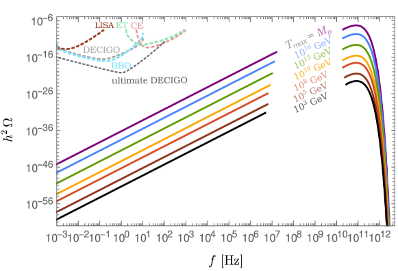
The authors of Drewes et al. (2024a) showed that refs. Ghiglieri and Laine (2015); Ringwald et al. (2021) have missed the suppression of the GW production rate on superhorizon scales. Including this suppression, one obtains the following Fig. 27 ,

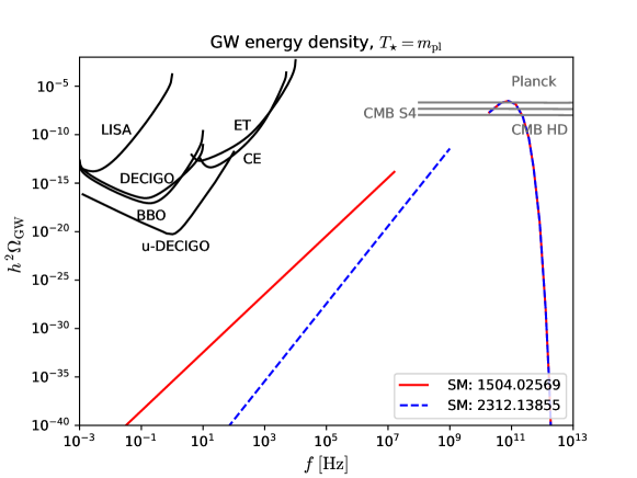
VII Conclusions

Gravitational wave cosmology is one of the most promising avenues for discovering physics beyond the Standard Model. Next-generation detectors promise to have cosmologically significant strain sensitivities over 12 decades of frequencies - from the nanoHz to the kHz. In section II we outlined three major strategies for gravitational wave detection - pulsar timing arrays, astrometry, and of course interferometry both terrestrial and in space.

In sections III-V we covered three very active subfields in gravitational cosmology which cover, in this review’s opinion, the three major sources that next-generation detectors will be sensitive to. First-order cosmic phase transitions can produce a source from the collision of bubbles, the explosion of sound, and the aftermath of turbulence. We surveyed the many possible scenarios that can produce a cosmological phase transition, though the electroweak phase transition continues to inspire the most interest. This source is arguably the most difficult to understand as it requires taming of finite temperature perturbation theory and understanding how the behaviour of bubbles and sound shells translates to precise predictions of spectra. So far, the community requires simulations to shed light on both issues and the theory is still maturing.

We covered an array of topological defects including hybrid defects in section IV. The string signals are expected to grow with the scale of spontaneous symmetry breaking, as is the cause of textures. Domain walls by contrast have a peak frequency and strength that is determined not just by the surface tension, but the lifetimes of the walls. In all three cases, there can be a detectable signal arising from physics at scales many orders of magnitude higher than what can be reached at the LHC. Successive symmetry-breaking steps can result in hybrid defects, with each possible combination having its own unique gravitational wave signature, indicating the possibility of learning about a potentially rich cosmic history. The most severe source of theoretical uncertainty is undoubtedly the mismatch between field-theoretic and string simulations of cosmic strings. This conflict appears to still be in flux and needs to be resolved. We conclude this section by discussing some of the applications of GW from topological defects.

Finally, in section V we considered scalar-induced gravitational waves. Despite being lumped under the same category, two radically different types of scenarios can result in scalar-induced gravitational waves - a period of ultra-slow roll inflation and a sudden change in the equation of state. Both sources have a theoretical uncertainty due to gauge invariance and it is hard to rigorously pin down the severity of this issue. There are, however, plausible arguments that we at least qualitatively understand the gravitational wave signal.

In the case of all three signals, there are no known mechanisms under which the Standard Model could provide the conditions needed to generate such a primordial source. So any detection of such a background would be a smoking gun of new physics. Moreover, all three sources potentially can involve physics at a higher scale than we can reach at the LHC. In the case of phase transitions, the frequency is loosely proportional to the scale of the transition, meaning that it is not a probe of very high-scale physics. However, the other two scenarios are less constrained. In the case of strings, the signal is expected to grow with the scale of symmetry breaking, whereas the peak frequency of signals from domain walls and resonantly enhanced scalar-induced gravitational waves corresponds to the lifetime of a macroscopic object. The range of applications to test high-scale physics is already quite broad and we expect it to grow over the next few decades.

There are other sources of gravitational waves, some of which we grouped together in section VI, which we only briefly summarized due to the fact that their detection is loosely connected to next-generation detectors such as inflation,²⁹²⁹29We say that is loosely connected rather than unconnected due to the possibility of a blue tilted spectrum or because the source is high frequency.

The discovery of gravitational waves has provided a method for observing the first moment of creating, where deficiencies in our understanding of what lies beyond the Standard Model matter the most. Gravitational wave cosmology is a new and rapidly growing field that has recently arisen in response to this challenge and opportunity and it feels as though we are just beginning to understand the potential of this field.

Acknowledgements. We are grateful to David Dunsky, Jessica Turner, Peter Athron, Carlos Tamarit, Yann Gouttenoire, Wenyuan Ai, Guillem Domenech and Qaisir Shafi for some useful discussions. GW acknowledge the STFC Consolidated Grant ST/L000296/1 and RR acknowledges financial support from the STFC Consolidated Grant ST/T000775/1.

References

Aasi et al. (2015) Aasi, J., et al. (LIGO Scientific) (2015), Class. Quant. Grav. 32, 074001, arXiv:1411.4547 [gr-qc] .
Abbott et al. (2016a) Abbott, B. P., et al. (LIGO Scientific, Virgo) (2016a), Phys. Rev. Lett. 116 (13), 131103, arXiv:1602.03838 [gr-qc] .
Abbott et al. (2016b) Abbott, B. P., et al. (LIGO Scientific, Virgo) (2016b), Phys. Rev. Lett. 116 (6), 061102, arXiv:1602.03837 [gr-qc] .
Abbott and Wise (1984) Abbott, L. F., and M. B. Wise (1984), Nucl. Phys. B 244, 541.
Abraham (1974) Abraham, F. F. (1974), Homogeneous nucleation theory, Vol. 263 (Elsevier).
Acernese et al. (2015) Acernese, F., et al. (VIRGO) (2015), Class. Quant. Grav. 32 (2), 024001, arXiv:1408.3978 [gr-qc] .
Acernese et al. (2019) Acernese, F., et al. (Virgo) (2019), Phys. Rev. Lett. 123 (23), 231108.
Adhikari et al. (2020) Adhikari, R. X., et al. (LIGO) (2020), Class. Quant. Grav. 37 (16), 165003, arXiv:2001.11173 [astro-ph.IM] .
Adshead et al. (2020a) Adshead, P., J. T. Giblin, M. Pieroni, and Z. J. Weiner (2020a), Phys. Rev. Lett. 124 (17), 171301, arXiv:1909.12843 [astro-ph.CO] .
Adshead et al. (2020b) Adshead, P., J. T. Giblin, M. Pieroni, and Z. J. Weiner (2020b), Phys. Rev. D 101 (8), 083534, arXiv:1909.12842 [astro-ph.CO] .
Adshead et al. (2018) Adshead, P., J. T. Giblin, and Z. J. Weiner (2018), Phys. Rev. D 98 (4), 043525, arXiv:1805.04550 [astro-ph.CO] .
Adshead et al. (2016) Adshead, P., E. Martinec, E. I. Sfakianakis, and M. Wyman (2016), JHEP 12, 137, arXiv:1609.04025 [hep-th] .
Adshead et al. (2013a) Adshead, P., E. Martinec, and M. Wyman (2013a), Phys. Rev. D 88 (2), 021302, arXiv:1301.2598 [hep-th] .
Adshead et al. (2013b) Adshead, P., E. Martinec, and M. Wyman (2013b), JHEP 09, 087, arXiv:1305.2930 [hep-th] .
Adshead and Sfakianakis (2017) Adshead, P., and E. I. Sfakianakis (2017), JHEP 08, 130, arXiv:1705.03024 [hep-th] .
Afzal et al. (2022) Afzal, A., W. Ahmed, M. U. Rehman, and Q. Shafi (2022), Phys. Rev. D 105 (10), 103539, arXiv:2202.07386 [hep-ph] .
Afzal et al. (2023a) Afzal, A., Q. Shafi, and A. Tiwari (2023a), arXiv:2311.05564 [hep-ph] .
Afzal et al. (2023b) Afzal, A., et al. (NANOGrav) (2023b), Astrophys. J. Lett. 951 (1), L11, arXiv:2306.16219 [astro-ph.HE] .
Agazie et al. (2023a) Agazie, G., et al. (NANOGrav) (2023a), Astrophys. J. Lett. 951 (1), L8, arXiv:2306.16213 [astro-ph.HE] .
Agazie et al. (2023b) Agazie, G., et al. (NANOGrav) (2023b), Astrophys. J. Lett. 951 (1), L9, arXiv:2306.16217 [astro-ph.HE] .
Aggarwal et al. (2021) Aggarwal, N., et al. (2021), Living Rev. Rel. 24 (1), 4, arXiv:2011.12414 [gr-qc] .
Aghanim et al. (2020a) Aghanim, N., et al. (Planck) (2020a), Astron. Astrophys. 641, A6, [Erratum: Astron.Astrophys. 652, C4 (2021)], arXiv:1807.06209 [astro-ph.CO] .
Aghanim et al. (2020b) Aghanim, N., et al. (Planck) (2020b), Astron. Astrophys. 641, A6, arXiv:1807.06209 [astro-ph.CO] .
Agrawal et al. (2023) Agrawal, P., S. Blasi, A. Mariotti, and M. Nee (2023), arXiv:2312.06749 [hep-ph] .
Ahmed et al. (2024) Ahmed, W., T. A. Chowdhury, S. Nasri, and S. Saad (2024), Phys. Rev. D 109 (1), 015008, arXiv:2308.13248 [hep-ph] .
Ahmed et al. (2022) Ahmed, W., M. Junaid, S. Nasri, and U. Zubair (2022), Phys. Rev. D 105 (11), 115008, arXiv:2202.06216 [hep-ph] .
Ahmed et al. (2023) Ahmed, W., M. U. Rehman, and U. Zubair (2023), arXiv:2308.09125 [hep-ph] .
Ahriche et al. (2019) Ahriche, A., K. Hashino, S. Kanemura, and S. Nasri (2019), Phys. Lett. B 789, 119, arXiv:1809.09883 [hep-ph] .
Ai (2023) Ai, W.-Y. (2023), arXiv:2308.10679 [hep-ph] .
Ai et al. (2022) Ai, W.-Y., B. Garbrecht, and C. Tamarit (2022), JCAP 03 (03), 015, arXiv:2109.13710 [hep-ph] .
Ai et al. (2023) Ai, W.-Y., B. Laurent, and J. van de Vis (2023), JCAP 07, 002, arXiv:2303.10171 [astro-ph.CO] .
Ai et al. (2024) Ai, W.-Y., X. Nagels, and M. Vanvlasselaer (2024), arXiv:2401.05911 [hep-ph] .
Akrami et al. (2020a) Akrami, Y., F. Arroja, M. Ashdown, J. Aumont, C. Baccigalupi, M. Ballardini, A. J. Banday, R. Barreiro, N. Bartolo, S. Basak, et al. (2020a), Astronomy & Astrophysics 641, A10.
Akrami et al. (2020b) Akrami, Y., et al. (Planck) (2020b), Astron. Astrophys. 641, A10, arXiv:1807.06211 [astro-ph.CO] .
Akutsu et al. (2019) Akutsu, T., et al. (KAGRA) (2019), Nature Astron. 3 (1), 35, arXiv:1811.08079 [gr-qc] .
Alabidi et al. (2013) Alabidi, L., K. Kohri, M. Sasaki, and Y. Sendouda (2013), Journal of Cosmology and Astroparticle Physics 2013 (05), 033.
Alanne et al. (2020) Alanne, T., N. Benincasa, M. Heikinheimo, K. Kannike, V. Keus, N. Koivunen, and K. Tuominen (2020), JHEP 10, 080, arXiv:2008.09605 [hep-ph] .
Albrecht and Steinhardt (1982) Albrecht, A., and P. J. Steinhardt (1982), Phys. Rev. Lett. 48, 1220.
Allahverdi et al. (2020) Allahverdi, R., M. A. Amin, A. Berlin, N. Bernal, C. T. Byrnes, M. S. Delos, A. L. Erickcek, M. Escudero, D. G. Figueroa, K. Freese, et al. (2020), arXiv preprint arXiv:2006.16182 .
Allahverdi et al. (2010) Allahverdi, R., R. Brandenberger, F.-Y. Cyr-Racine, and A. Mazumdar (2010), Ann. Rev. Nucl. Part. Sci. 60, 27, arXiv:1001.2600 [hep-th] .
Allen and Shellard (1992) Allen, B., and E. P. S. Shellard (1992), Phys. Rev. D 45, 1898.
Altarelli and Isidori (1994) Altarelli, G., and G. Isidori (1994), Phys. Lett. B 337, 141.
Alves et al. (2019) Alves, A., T. Ghosh, H.-K. Guo, K. Sinha, and D. Vagie (2019), JHEP 04, 052, arXiv:1812.09333 [hep-ph] .
Amaro-Seoane et al. (2017) Amaro-Seoane, P., et al. (LISA) (2017), arXiv:1702.00786 [astro-ph.IM] .
Amin (2013) Amin, M. A. (2013), Physical Review D 87 (12), 123505.
Amin et al. (2010) Amin, M. A., R. Easther, and H. Finkel (2010), Journal of Cosmology and Astroparticle Physics 2010 (12), 001.
Amin et al. (2012) Amin, M. A., R. Easther, H. Finkel, R. Flauger, and M. P. Hertzberg (2012), Physical review letters 108 (24), 241302.
Amin and Shirokoff (2010) Amin, M. A., and D. Shirokoff (2010), Physical Review D 81 (8), 085045.
Anber and Sorbo (2012) Anber, M. M., and L. Sorbo (2012), Phys. Rev. D 85, 123537, arXiv:1203.5849 [astro-ph.CO] .
Andersen et al. (2018) Andersen, J. O., T. Gorda, A. Helset, L. Niemi, T. V. I. Tenkanen, A. Tranberg, A. Vuorinen, and D. J. Weir (2018), Phys. Rev. Lett. 121 (19), 191802, arXiv:1711.09849 [hep-ph] .
Ando et al. (2018a) Ando, K., K. Inomata, M. Kawasaki, K. Mukaida, and T. T. Yanagida (2018a), Physical Review D 97 (12), 123512.
Ando et al. (2018b) Ando, K., M. Kawasaki, and H. Nakatsuka (2018b), Physical Review D 98 (8), 083508.
Angelescu and Huang (2019) Angelescu, A., and P. Huang (2019), Phys. Rev. D 99 (5), 055023, arXiv:1812.08293 [hep-ph] .
Anisha et al. (2022) Anisha,, L. Biermann, C. Englert, and M. Mühlleitner (2022), JHEP 08, 091, arXiv:2204.06966 [hep-ph] .
Antoniadis et al. (2023a) Antoniadis, J., et al. (EPTA) (2023a), Astron. Astrophys. 678, A48, arXiv:2306.16224 [astro-ph.HE] .
Antoniadis et al. (2023b) Antoniadis, J., et al. (2023b), arXiv:2306.16214 [astro-ph.HE] .
Antoniadis et al. (2023c) Antoniadis, J., et al. (2023c), arXiv:2306.16227 [astro-ph.CO] .
Antusch et al. (2018a) Antusch, S., F. Cefala, S. Krippendorf, F. Muia, S. Orani, and F. Quevedo (2018a), Journal of High Energy Physics 2018 (1), 1.
Antusch et al. (2016) Antusch, S., F. Cefala, D. Nolde, and S. Orani (2016), Journal of Cosmology and Astroparticle Physics 2016 (02), 044.
Antusch et al. (2017) Antusch, S., F. Cefala, and S. Orani (2017), Physical Review Letters 118 (1), 011303.
Antusch et al. (2018b) Antusch, S., F. Cefala, and S. Orani (2018b), Journal of Cosmology and Astroparticle Physics 2018 (03), 032.
Antusch et al. (2019) Antusch, S., F. Cefala, and F. Torrenti (2019), Journal of Cosmology and Astroparticle Physics 2019 (10), 002.
Antusch et al. (2023) Antusch, S., K. Hinze, S. Saad, and J. Steiner (2023), Phys. Rev. D 108 (9), 095053, arXiv:2307.04595 [hep-ph] .
Antusch and Orani (2016) Antusch, S., and S. Orani (2016), Journal of Cosmology and Astroparticle Physics 2016 (03), 026.
Aoki et al. (2022) Aoki, M., T. Komatsu, and H. Shibuya (2022), PTEP 2022 (6), 063B05, arXiv:2106.03439 [hep-ph] .
Aoki and Kubo (2020) Aoki, M., and J. Kubo (2020), JCAP 04, 001, arXiv:1910.05025 [hep-ph] .
Aoki et al. (2006) Aoki, Y., G. Endrodi, Z. Fodor, S. D. Katz, and K. K. Szabo (2006), Nature 443, 675, arXiv:hep-lat/0611014 .
Appelquist and Pisarski (1981) Appelquist, T., and R. D. Pisarski (1981), Phys. Rev. D 23, 2305.
Apreda et al. (2002) Apreda, R., M. Maggiore, A. Nicolis, and A. Riotto (2002), Nucl. Phys. B 631, 342, arXiv:gr-qc/0107033 .
Arbey and Mahmoudi (2021) Arbey, A., and F. Mahmoudi (2021), Progress in Particle and Nuclear Physics 119, 103865.
Arcadi et al. (2023) Arcadi, G., N. Benincasa, A. Djouadi, and K. Kannike (2023), Phys. Rev. D 108 (5), 055010, arXiv:2212.14788 [hep-ph] .
Arnold (1989) Arnold, P. B. (1989), Phys. Rev. D 40, 613.
Arun et al. (2017) Arun, K., S. Gudennavar, and C. Sivaram (2017), Advances in Space Research 60 (1), 166.
Ashoorioon et al. (2021) Ashoorioon, A., A. Rostami, and J. T. Firouzjaee (2021), Journal of High Energy Physics 2021 (7), 1.
Aso et al. (2013) Aso, Y., Y. Michimura, K. Somiya, M. Ando, O. Miyakawa, T. Sekiguchi, D. Tatsumi, and H. Yamamoto (KAGRA) (2013), Phys. Rev. D 88 (4), 043007, arXiv:1306.6747 [gr-qc] .
Astros et al. (2023) Astros, M. D., S. Fabian, and F. Goertz (2023), arXiv:2307.01270 [hep-ph] .
Atal and Domènech (2021) Atal, V., and G. Domènech (2021), Journal of Cosmology and Astroparticle Physics 2021 (06), 001.
Atal and Germani (2019) Atal, V., and C. Germani (2019), Physics of the Dark Universe 24, 100275.
Athron et al. (2023a) Athron, P., C. Balázs, A. Fowlie, L. Morris, and L. Wu (2023a), arXiv:2305.02357 [hep-ph] .
Athron et al. (2023b) Athron, P., C. Balázs, T. E. Gonzalo, and M. Pearce (2023b), arXiv:2307.02544 [hep-ph] .
Athron et al. (2023c) Athron, P., L. Morris, and Z. Xu (2023c), arXiv:2309.05474 [hep-ph] .
Atkinson et al. (2022) Atkinson, O., M. Black, C. Englert, A. Lenz, A. Rusov, and J. Wynne (2022), JHEP 11, 139, arXiv:2202.08807 [hep-ph] .
Auclair et al. (2022) Auclair, P., C. Caprini, D. Cutting, M. Hindmarsh, K. Rummukainen, D. A. Steer, and D. J. Weir (2022), JCAP 09, 029, arXiv:2205.02588 [astro-ph.CO] .
Auclair et al. (2020) Auclair, P., et al. (2020), JCAP 2004, 034, arXiv:1909.00819 [astro-ph.CO] .
Aufmuth and Danzmann (2005) Aufmuth, P., and K. Danzmann (2005), New J. Phys. 7, 202.
Avelino et al. (2005) Avelino, P. P., C. J. A. P. Martins, and J. C. R. E. Oliveira (2005), Phys. Rev. D 72, 083506, arXiv:hep-ph/0507272 .
Azatov et al. (2023) Azatov, A., G. Barni, R. Petrossian-Byrne, and M. Vanvlasselaer (2023), arXiv:2310.06972 [hep-ph] .
Azatov and Vanvlasselaer (2021) Azatov, A., and M. Vanvlasselaer (2021), JCAP 01, 058, arXiv:2010.02590 [hep-ph] .
Azatov et al. (2021) Azatov, A., M. Vanvlasselaer, and W. Yin (2021), JHEP 10, 043, arXiv:2106.14913 [hep-ph] .
Balazs (2014) Balazs, C. (2014), arXiv preprint arXiv:1411.3398 .
Balazs et al. (2017) Balazs, C., G. White, and J. Yue (2017), JHEP 03, 030, arXiv:1612.01270 [hep-ph] .
Baldes (2017) Baldes, I. (2017), JCAP 05, 028, arXiv:1702.02117 [hep-ph] .
Baldes et al. (2021a) Baldes, I., S. Blasi, A. Mariotti, A. Sevrin, and K. Turbang (2021a), Phys. Rev. D 104 (11), 115029, arXiv:2106.15602 [hep-ph] .
Baldes and Garcia-Cely (2019) Baldes, I., and C. Garcia-Cely (2019), JHEP 05, 190, arXiv:1809.01198 [hep-ph] .
Baldes et al. (2021b) Baldes, I., Y. Gouttenoire, and F. Sala (2021b), JHEP 04, 278, arXiv:2007.08440 [hep-ph] .
Ballesteros and Taoso (2018) Ballesteros, G., and M. Taoso (2018), Phys. Rev. D 97 (2), 023501, arXiv:1709.05565 [hep-ph] .
Banks and Dixon (1988) Banks, T., and L. J. Dixon (1988), Nucl. Phys. B 307, 93.
Banks and Seiberg (2011) Banks, T., and N. Seiberg (2011), Phys. Rev. D 83, 084019, arXiv:1011.5120 [hep-th] .
Barman et al. (2022a) Barman, B., D. Borah, S. J. Das, and R. Roshan (2022a), JCAP 03 (03), 031, arXiv:2111.08034 [hep-ph] .
Barman et al. (2022b) Barman, B., D. Borah, S. Das Jyoti, and R. Roshan (2022b), JCAP 08, 068, arXiv:2204.10339 [hep-ph] .
Barman et al. (2023a) Barman, B., D. Borah, S. Jyoti Das, and R. Roshan (2023a), Phys. Rev. D 107 (9), 095002, arXiv:2212.00052 [hep-ph] .
Barman et al. (2023b) Barman, B., D. Borah, S. Jyoti Das, and I. Saha (2023b), JCAP 10, 053, arXiv:2307.00656 [hep-ph] .
Barroso Mancha et al. (2021) Barroso Mancha, M., T. Prokopec, and B. Swiezewska (2021), JHEP 01, 070, arXiv:2005.10875 [hep-th] .
Barrow et al. (1991) Barrow, J. D., E. J. Copeland, E. W. Kolb, and A. R. Liddle (1991), Phys. Rev. D 43, 984.
Basilakos et al. (2024a) Basilakos, S., D. V. Nanopoulos, T. Papanikolaou, E. N. Saridakis, and C. Tzerefos (2024a), Phys. Lett. B 850, 138507, arXiv:2307.08601 [hep-th] .
Basilakos et al. (2024b) Basilakos, S., D. V. Nanopoulos, T. Papanikolaou, E. N. Saridakis, and C. Tzerefos (2024b), Phys. Lett. B 849, 138446, arXiv:2309.15820 [astro-ph.CO] .
Basler et al. (2017) Basler, P., M. Krause, M. Muhlleitner, J. Wittbrodt, and A. Wlotzka (2017), JHEP 02, 121, arXiv:1612.04086 [hep-ph] .
Bassett et al. (2006) Bassett, B. A., S. Tsujikawa, and D. Wands (2006), Reviews of Modern Physics 78 (2), 537.
Battye and Shellard (1996) Battye, R. A., and E. P. S. Shellard (1996), arXiv:astro-ph/9604059 [astro-ph] .
Battye and Shellard (1997) Battye, R. A., and E. P. S. Shellard (1997), in 1st International Heidelberg Conference on Dark Matter in Astro and Particle Physics, pp. 554–579, arXiv:astro-ph/9706014 .
Baum et al. (2021) Baum, S., M. Carena, N. R. Shah, C. E. M. Wagner, and Y. Wang (2021), JHEP 03, 055, arXiv:2009.10743 [hep-ph] .
Baumann et al. (2007) Baumann, D., P. J. Steinhardt, and N. Turok (2007), arXiv:hep-th/0703250 .
Bazavov et al. (2017) Bazavov, A., et al. (2017), Phys. Rev. D 95 (5), 054504, arXiv:1701.04325 [hep-lat] .
Bednyakov et al. (2015) Bednyakov, A. V., B. A. Kniehl, A. F. Pikelner, and O. L. Veretin (2015), Phys. Rev. Lett. 115 (20), 201802, arXiv:1507.08833 [hep-ph] .
Benincasa et al. (2022) Benincasa, N., L. Delle Rose, K. Kannike, and L. Marzola (2022), JCAP 12, 025, arXiv:2205.06669 [hep-ph] .
Benincasa et al. (2023) Benincasa, N., A. Hryczuk, K. Kannike, and M. Laletin (2023), arXiv:2312.04627 [hep-ph] .
Beniwal et al. (2019) Beniwal, A., M. Lewicki, M. White, and A. G. Williams (2019), JHEP 02, 183, arXiv:1810.02380 [hep-ph] .
Bento (2003) Bento, L. (2003), JCAP 11, 002, arXiv:hep-ph/0304263 .
Bergström (2000) Bergström, L. (2000), Rept. Prog. Phys. 63, 793, arXiv:hep-ph/0002126 .
Bernon et al. (2018) Bernon, J., L. Bian, and Y. Jiang (2018), JHEP 05, 151, arXiv:1712.08430 [hep-ph] .
Bertone and Hooper (2018) Bertone, G., and D. Hooper (2018), Rev. Mod. Phys. 90 (4), 045002, arXiv:1605.04909 [astro-ph.CO] .
Bertone et al. (2005) Bertone, G., D. Hooper, and J. Silk (2005), Phys. Rept. 405, 279, arXiv:hep-ph/0404175 .
Bertone and Tait (2018) Bertone, G., and T. M. Tait (2018), Nature 562 (7725), 51.
Bezrukov et al. (2012) Bezrukov, F., M. Y. Kalmykov, B. A. Kniehl, and M. Shaposhnikov (2012), JHEP 10, 140, arXiv:1205.2893 [hep-ph] .
Bhattacharya et al. (2023a) Bhattacharya, G., S. Choudhury, K. Dey, S. Ghosh, A. Karde, and N. S. Mishra (2023a), arXiv:2309.00973 [astro-ph.CO] .
Bhattacharya et al. (2023b) Bhattacharya, S., N. Mondal, R. Roshan, and D. Vatsyayan (2023b), arXiv:2312.15053 [hep-ph] .
Bhattacharya et al. (2021) Bhattacharya, S., R. Roshan, A. Sil, and D. Vatsyayan (2021), arXiv:2105.06189 [hep-ph] .
Bhattacharya et al. (2014) Bhattacharya, T., et al. (2014), Phys. Rev. Lett. 113 (8), 082001, arXiv:1402.5175 [hep-lat] .
Bhaumik et al. (2023) Bhaumik, N., A. Ghoshal, R. K. Jain, and M. Lewicki (2023), JHEP 05, 169, arXiv:2212.00775 [astro-ph.CO] .
Bhaumik et al. (2022) Bhaumik, N., A. Ghoshal, and M. Lewicki (2022), JHEP 07, 130, arXiv:2205.06260 [astro-ph.CO] .
Bhaumik and Jain (2021) Bhaumik, N., and R. K. Jain (2021), Phys. Rev. D 104 (2), 023531, arXiv:2009.10424 [astro-ph.CO] .
Biagetti et al. (2013) Biagetti, M., M. Fasiello, and A. Riotto (2013), Phys. Rev. D 88, 103518, arXiv:1305.7241 [astro-ph.CO] .
Bian et al. (2021) Bian, L., W. Cheng, H.-K. Guo, and Y. Zhang (2021), Chin. Phys. C 45 (11), 113104, arXiv:1907.13589 [hep-ph] .
Bian et al. (2018) Bian, L., H.-K. Guo, and J. Shu (2018), Chin. Phys. C 42 (9), 093106, [Erratum: Chin.Phys.C 43, 129101 (2019)], arXiv:1704.02488 [hep-ph] .
Bian et al. (2019) Bian, L., Y. Wu, and K.-P. Xie (2019), JHEP 12, 028, arXiv:1909.02014 [hep-ph] .
Biekötter et al. (2021) Biekötter, T., S. Heinemeyer, J. M. No, M. O. Olea, and G. Weiglein (2021), JCAP 06, 018, arXiv:2103.12707 [hep-ph] .
Biekötter et al. (2023a) Biekötter, T., S. Heinemeyer, J. M. No, M. O. Olea-Romacho, and G. Weiglein (2023a), JCAP 03, 031, arXiv:2208.14466 [hep-ph] .
Biekötter et al. (2023b) Biekötter, T., S. Heinemeyer, J. M. No, K. Radchenko, M. O. O. Romacho, and G. Weiglein (2023b), arXiv:2309.17431 [hep-ph] .
Bigazzi et al. (2020) Bigazzi, F., A. Caddeo, A. L. Cotrone, and A. Paredes (2020), JHEP 12, 200, arXiv:2008.02579 [hep-th] .
Bigazzi et al. (2021) Bigazzi, F., A. Caddeo, A. L. Cotrone, and A. Paredes (2021), JHEP 04, 094, arXiv:2011.08757 [hep-ph] .
Blanco-Pillado et al. (2023) Blanco-Pillado, J. J., D. Jiménez-Aguilar, J. Lizarraga, A. Lopez-Eiguren, K. D. Olum, A. Urio, and J. Urrestilla (2023), JCAP 05, 035, arXiv:2302.03717 [hep-th] .
Blanco-Pillado and Olum (2017) Blanco-Pillado, J. J., and K. D. Olum (2017), Phys. Rev. D 96 (10), 104046, arXiv:1709.02693 [astro-ph.CO] .
Blanco-Pillado et al. (2011a) Blanco-Pillado, J. J., K. D. Olum, and B. Shlaer (2011a), Phys. Rev. D 83, 083514, arXiv:1101.5173 [astro-ph.CO] .
Blanco-Pillado et al. (2011b) Blanco-Pillado, J. J., K. D. Olum, and B. Shlaer (2011b), Phys. Rev. D83, 083514, arXiv:1101.5173 [astro-ph.CO] .
Blanco-Pillado et al. (2014) Blanco-Pillado, J. J., K. D. Olum, and B. Shlaer (2014), Phys. Rev. D89 (2), 023512, arXiv:1309.6637 [astro-ph.CO] .
Blas and Jenkins (2022a) Blas, D., and A. C. Jenkins (2022a), Phys. Rev. Lett. 128 (10), 101103, arXiv:2107.04601 [astro-ph.CO] .
Blas and Jenkins (2022b) Blas, D., and A. C. Jenkins (2022b), Phys. Rev. D 105 (6), 064021, arXiv:2107.04063 [gr-qc] .
Blasi et al. (2020) Blasi, S., V. Brdar, and K. Schmitz (2020), Phys. Rev. Res. 2 (4), 043321, arXiv:2004.02889 [hep-ph] .
Blasi et al. (2023a) Blasi, S., R. Jinno, T. Konstandin, H. Rubira, and I. Stomberg (2023a), JCAP 10, 051, arXiv:2302.06952 [astro-ph.CO] .
Blasi and Mariotti (2022) Blasi, S., and A. Mariotti (2022), Phys. Rev. Lett. 129 (26), 261303, arXiv:2203.16450 [hep-ph] .
Blasi et al. (2023b) Blasi, S., A. Mariotti, A. Rase, and A. Sevrin (2023b), JHEP 11, 169, arXiv:2306.17830 [hep-ph] .
Blasi et al. (2023c) Blasi, S., A. Mariotti, A. Rase, A. Sevrin, and K. Turbang (2023c), JCAP 04, 008, arXiv:2210.14246 [hep-ph] .
Blinov et al. (2015a) Blinov, N., J. Kozaczuk, D. E. Morrissey, and C. Tamarit (2015a), Phys. Rev. D 92 (3), 035012, arXiv:1504.05195 [hep-ph] .
Blinov et al. (2015b) Blinov, N., S. Profumo, and T. Stefaniak (2015b), JCAP 07, 028, arXiv:1504.05949 [hep-ph] .
Blum (2022) Blum, A. S. (2022), Archive for History of Exact Sciences 76 (6), 623.
Bodeker and Buchmuller (2021) Bodeker, D., and W. Buchmuller (2021), Rev. Mod. Phys. 93 (3), 035004, arXiv:2009.07294 [hep-ph] .
Bodeker et al. (2005) Bodeker, D., L. Fromme, S. J. Huber, and M. Seniuch (2005), JHEP 02, 026, arXiv:hep-ph/0412366 .
Bodeker et al. (1997) Bodeker, D., P. John, M. Laine, and M. G. Schmidt (1997), Nucl. Phys. B 497, 387, arXiv:hep-ph/9612364 .
Bodeker and Moore (2009) Bodeker, D., and G. D. Moore (2009), JCAP 0905, 009, arXiv:0903.4099 [hep-ph] .
Bodeker and Moore (2017) Bodeker, D., and G. D. Moore (2017), JCAP 05, 025, arXiv:1703.08215 [hep-ph] .
Boehm et al. (2017) Boehm, C., et al. (Theia) (2017), arXiv:1707.01348 [astro-ph.IM] .
Book and Flanagan (2011) Book, L. G., and E. E. Flanagan (2011), Phys. Rev. D 83, 024024, arXiv:1009.4192 [astro-ph.CO] .
Borah et al. (2022) Borah, D., S. Jyoti Das, and R. Roshan (2022), arXiv:2208.04965 [hep-ph] .
Borah et al. (2023) Borah, D., S. Jyoti Das, R. Roshan, and R. Samanta (2023), Phys. Rev. D 108 (2), 023531, arXiv:2304.11844 [hep-ph] .
Bosch et al. (2023) Bosch, J., Z. Delgado, B. Fornal, and A. Leon (2023), arXiv:2306.00332 [hep-ph] .
Boyanovsky et al. (2006) Boyanovsky, D., H. De Vega, and D. Schwarz (2006), Annu. Rev. Nucl. Part. Sci. 56, 441.
Boyd et al. (1993a) Boyd, C. G., D. E. Brahm, and S. D. H. Hsu (1993a), Phys. Rev. D 48, 4952, arXiv:hep-ph/9206235 .
Boyd et al. (1993b) Boyd, C. G., D. E. Brahm, and S. D. H. Hsu (1993b), Phys. Rev. D 48, 4963, arXiv:hep-ph/9304254 .
Braaten and Nieto (1995) Braaten, E., and A. Nieto (1995), Phys. Rev. D 51, 6990, arXiv:hep-ph/9501375 .
Braaten and Nieto (1996) Braaten, E., and A. Nieto (1996), Phys. Rev. D 53, 3421, arXiv:hep-ph/9510408 .
Brdar et al. (2019a) Brdar, V., L. Graf, A. J. Helmboldt, and X.-J. Xu (2019a), JCAP 12, 027, arXiv:1909.02018 [hep-ph] .
Brdar et al. (2019b) Brdar, V., A. J. Helmboldt, and J. Kubo (2019b), JCAP 02, 021, arXiv:1810.12306 [hep-ph] .
Breitbach et al. (2019) Breitbach, M., J. Kopp, E. Madge, T. Opferkuch, and P. Schwaller (2019), JCAP 07, 007, arXiv:1811.11175 [hep-ph] .
Brown et al. (2018) Brown, A. G. A., et al. (Gaia) (2018), Astron. Astrophys. 616, A1, arXiv:1804.09365 [astro-ph.GA] .
Brustein et al. (1995) Brustein, R., M. Gasperini, M. Giovannini, and G. Veneziano (1995), arXiv preprint hep-th/9510081 .
Buchmuller et al. (2021) Buchmuller, W., V. Domcke, and K. Schmitz (2021), “Stochastic gravitational-wave background from metastable cosmic strings,” arXiv:2107.04578 [hep-ph] .
Buchmuller et al. (2023) Buchmuller, W., V. Domcke, and K. Schmitz (2023), JCAP 11, 020, arXiv:2307.04691 [hep-ph] .
Bugaev et al. (2003) Bugaev, E. V., M. G. Elbakidze, and K. V. Konishchev (2003), Phys. Atom. Nucl. 66, 476, arXiv:astro-ph/0110660 .
Buikema et al. (2020) Buikema, A., et al. (aLIGO) (2020), Phys. Rev. D 102 (6), 062003, arXiv:2008.01301 [astro-ph.IM] .
Burke-Spolaor et al. (2019) Burke-Spolaor, S., et al. (2019), Astron. Astrophys. Rev. 27 (1), 5, arXiv:1811.08826 [astro-ph.HE] .
Buttazzo et al. (2013) Buttazzo, D., G. Degrassi, P. P. Giardino, G. F. Giudice, F. Sala, A. Salvio, and A. Strumia (2013), JHEP 12, 089, arXiv:1307.3536 [hep-ph] .
Byrnes et al. (2019) Byrnes, C. T., P. S. Cole, and S. P. Patil (2019), Journal of Cosmology and Astroparticle Physics 2019 (06), 028.
Cai et al. (2019) Cai, Y.-F., C. Chen, X. Tong, D.-G. Wang, and S.-F. Yan (2019), Physical Review D 100 (4), 043518.
Cai et al. (2018) Cai, Y.-F., X. Tong, D.-G. Wang, and S.-F. Yan (2018), Physical Review Letters 121 (8), 081306.
Caldwell and Devulder (2018) Caldwell, R. R., and C. Devulder (2018), Phys. Rev. D 97 (2), 023532, arXiv:1706.03765 [astro-ph.CO] .
Callan Jr and Coleman (1977) Callan Jr, C. G., and S. Coleman (1977), Physical Review D 16 (6), 1762.
Câmara Pereira et al. (2020) Câmara Pereira, R., J. a. Moreira, and P. Costa (2020), Eur. Phys. J. A 56 (8), 214, arXiv:2006.02385 [hep-ph] .
Canetti et al. (2012) Canetti, L., M. Drewes, and M. Shaposhnikov (2012), New J. Phys. 14, 095012, arXiv:1204.4186 [hep-ph] .
Cang et al. (2023a) Cang, J., Y. Gao, Y. Liu, and S. Sun (2023a), arXiv:2309.15069 [astro-ph.CO] .
Cang et al. (2023b) Cang, J., Y.-Z. Ma, and Y. Gao (2023b), Astrophys. J. 949 (2), 64, arXiv:2210.03476 [astro-ph.CO] .
Cao et al. (2022) Cao, Q.-H., K. Hashino, X.-X. Li, and J.-H. Yue (2022), arXiv:2212.07756 [hep-ph] .
Caprini et al. (2020a) Caprini, C., M. Chala, G. C. Dorsch, M. Hindmarsh, S. J. Huber, T. Konstandin, J. Kozaczuk, G. Nardini, J. M. No, K. Rummukainen, et al. (2020a), Journal of Cosmology and Astroparticle Physics 2020 (03), 024.
Caprini et al. (2009a) Caprini, C., R. Durrer, T. Konstandin, and G. Servant (2009a), Phys. Rev. D79, 083519, arXiv:0901.1661 [astro-ph.CO] .
Caprini et al. (2008) Caprini, C., R. Durrer, and G. Servant (2008), Phys. Rev. D 77, 124015, arXiv:0711.2593 [astro-ph] .
Caprini et al. (2009b) Caprini, C., R. Durrer, and G. Servant (2009b), JCAP 0912, 024, arXiv:0909.0622 [astro-ph.CO] .
Caprini et al. (2010) Caprini, C., R. Durrer, and X. Siemens (2010), Phys. Rev. D 82, 063511, arXiv:1007.1218 [astro-ph.CO] .
Caprini et al. (2020b) Caprini, C., et al. (2020b), JCAP 03, 024, arXiv:1910.13125 [astro-ph.CO] .
Carena et al. (2009) Carena, M., G. Nardini, M. Quiros, and C. E. M. Wagner (2009), Nucl. Phys. B 812, 243, arXiv:0809.3760 [hep-ph] .
Carena et al. (2013) Carena, M., G. Nardini, M. Quiros, and C. E. M. Wagner (2013), JHEP 02, 001, arXiv:1207.6330 [hep-ph] .
Carena et al. (1996) Carena, M., M. Quiros, and C. E. M. Wagner (1996), Phys. Lett. B 380, 81, arXiv:hep-ph/9603420 .
de Carlos and Espinosa (1997) de Carlos, B., and J. R. Espinosa (1997), Nucl. Phys. B 503, 24, arXiv:hep-ph/9703212 .
Carr et al. (2021) Carr, B., K. Kohri, Y. Sendouda, and J. Yokoyama (2021), Rept. Prog. Phys. 84 (11), 116902, arXiv:2002.12778 [astro-ph.CO] .
Carr and Kuhnel (2020) Carr, B., and F. Kuhnel (2020), Ann. Rev. Nucl. Part. Sci. 70, 355, arXiv:2006.02838 [astro-ph.CO] .
Carr et al. (2016) Carr, B., F. Kuhnel, and M. Sandstad (2016), Phys. Rev. D 94 (8), 083504, arXiv:1607.06077 [astro-ph.CO] .
Carr (1975) Carr, B. J. (1975), Astrophys. J. 201, 1.
Casas et al. (1996) Casas, J. A., J. R. Espinosa, and M. Quiros (1996), Phys. Lett. B 382, 374, arXiv:hep-ph/9603227 .
Çalışkan et al. (2023) Çalışkan, M., Y. Chen, L. Dai, N. Anil Kumar, I. Stomberg, and X. Xue (2023), arXiv:2312.03069 [gr-qc] .
Chala et al. (2018) Chala, M., C. Krause, and G. Nardini (2018), JHEP 07, 062, arXiv:1802.02168 [hep-ph] .
Chala et al. (2019) Chala, M., M. Ramos, and M. Spannowsky (2019), Eur. Phys. J. C 79 (2), 156, arXiv:1812.01901 [hep-ph] .
Chang and Cui (2020) Chang, C.-F., and Y. Cui (2020), Phys. Dark Univ. 29, 100604, arXiv:1910.04781 [hep-ph] .
Chang and Cui (2022) Chang, C.-F., and Y. Cui (2022), JHEP 03, 114, arXiv:2106.09746 [hep-ph] .
Chang et al. (2021) Chang, Z., S. Wang, and Q.-H. Zhu (2021), Chin. Phys. C 45 (9), 095101, arXiv:2009.11025 [astro-ph.CO] .
Chao et al. (2020) Chao, W., W.-F. Cui, H.-K. Guo, and J. Shu (2020), Chin. Phys. C 44 (12), 123102, arXiv:1707.09759 [hep-ph] .
Chao et al. (2017) Chao, W., H.-K. Guo, and J. Shu (2017), arXiv:1702.02698 [hep-ph] .
Chao et al. (2021) Chao, W., X.-F. Li, and L. Wang (2021), JCAP 06, 038, arXiv:2012.15113 [hep-ph] .
Chen and Cai (2019) Chen, C., and Y.-F. Cai (2019), Journal of Cosmology and Astroparticle Physics 2019 (10), 068.
Chen et al. (2020a) Chen, C., X.-H. Ma, and Y.-F. Cai (2020a), Physical Review D 102 (6), 063526.
Chen et al. (2020b) Chen, N., T. Li, Y. Wu, and L. Bian (2020b), Phys. Rev. D 101 (7), 075047, arXiv:1911.05579 [hep-ph] .
Chen et al. (2019) Chen, X., D. Li, and M. Huang (2019), Chinese Physics C 43 (2), 023105.
Chiang and Lu (2021) Chiang, C.-W., and B.-Q. Lu (2021), JCAP 05, 049, arXiv:2012.14071 [hep-ph] .
Chiang et al. (2018) Chiang, C.-W., M. J. Ramsey-Musolf, and E. Senaha (2018), Phys. Rev. D 97 (1), 015005, arXiv:1707.09960 [hep-ph] .
Child and Giblin (2012) Child, H. L., and J. T. Giblin, Jr. (2012), JCAP 10, 001, arXiv:1207.6408 [astro-ph.CO] .
Cho et al. (2021) Cho, G.-C., C. Idegawa, and E. Senaha (2021), Phys. Lett. B 823, 136787, arXiv:2105.11830 [hep-ph] .
Choudhury et al. (2023a) Choudhury, S., K. Dey, and A. Karde (2023a), arXiv:2311.15065 [astro-ph.CO] .
Choudhury et al. (2023b) Choudhury, S., M. R. Gangopadhyay, and M. Sami (2023b), arXiv:2301.10000 [astro-ph.CO] .
Choudhury et al. (2023c) Choudhury, S., S. Panda, and M. Sami (2023c), JCAP 08, 078, arXiv:2304.04065 [astro-ph.CO] .
Choudhury et al. (2023d) Choudhury, S., S. Panda, and M. Sami (2023d), Phys. Lett. B 845, 138123, arXiv:2302.05655 [astro-ph.CO] .
Choudhury et al. (2023e) Choudhury, S., S. Panda, and M. Sami (2023e), JCAP 11, 066, arXiv:2303.06066 [astro-ph.CO] .
Chung et al. (2013) Chung, D. J. H., A. J. Long, and L.-T. Wang (2013), Phys. Rev. D 87 (2), 023509, arXiv:1209.1819 [hep-ph] .
Clarkson and Seahra (2007) Clarkson, C., and S. S. Seahra (2007), Classical and Quantum Gravity 24 (9), F33.
Cline (2006) Cline, J. M. (2006), in Les Houches Summer School - Session 86: Particle Physics and Cosmology: The Fabric of Spacetime, arXiv:hep-ph/0609145 .
Cline et al. (2021) Cline, J. M., A. Friedlander, D.-M. He, K. Kainulainen, B. Laurent, and D. Tucker-Smith (2021), Phys. Rev. D 103 (12), 123529, arXiv:2102.12490 [hep-ph] .
Cline and Kainulainen (1996) Cline, J. M., and K. Kainulainen (1996), Nucl. Phys. B 482, 73, arXiv:hep-ph/9605235 .
Cline and Kainulainen (2013) Cline, J. M., and K. Kainulainen (2013), JCAP 1301, 012, arXiv:1210.4196 [hep-ph] .
Cline et al. (2013) Cline, J. M., K. Kainulainen, P. Scott, and C. Weniger (2013), Phys. Rev. D88, 055025, [Erratum: Phys. Rev.D92,no.3,039906(2015)], arXiv:1306.4710 [hep-ph] .
Cline et al. (2009) Cline, J. M., G. Laporte, H. Yamashita, and S. Kraml (2009), JHEP 07, 040, arXiv:0905.2559 [hep-ph] .
Cline and Moore (1998) Cline, J. M., and G. D. Moore (1998), Phys. Rev. Lett. 81, 3315, arXiv:hep-ph/9806354 .
Coleman (1977) Coleman, S. (1977), Physical Review D 15 (10), 2929.
Cook and Sorbo (2012) Cook, J. L., and L. Sorbo (2012), Phys. Rev. D 85, 023534, [Erratum: Phys.Rev.D 86, 069901 (2012)], arXiv:1109.0022 [astro-ph.CO] .
Copeland et al. (2004) Copeland, E. J., R. C. Myers, and J. Polchinski (2004), JHEP 06, 013, arXiv:hep-th/0312067 [hep-th] .
Correia and Martins (2019) Correia, J. R. C. C. C., and C. J. A. P. Martins (2019), Phys. Rev. D 100 (10), 103517, arXiv:1911.03163 [astro-ph.CO] .
Costa et al. (2022a) Costa, F., S. Khan, and J. Kim (2022a), JHEP 06, 026, arXiv:2202.13126 [hep-ph] .
Costa et al. (2022b) Costa, F., S. Khan, and J. Kim (2022b), JHEP 12, 165, arXiv:2209.13653 [hep-ph] .
Costa et al. (2009) Costa, P., C. A. de Sousa, M. C. Ruivo, and H. Hansen (2009), EPL 86 (3), 31001, arXiv:0801.3616 [hep-ph] .
Craig et al. (2020) Craig, N., N. Levi, A. Mariotti, and D. Redigolo (2020), JHEP 21, 184, arXiv:2011.13949 [hep-ph] .
Croon et al. (2019a) Croon, D., T. E. Gonzalo, and G. White (2019a), JHEP 02, 083, arXiv:1812.02747 [hep-ph] .
Croon et al. (2021) Croon, D., O. Gould, P. Schicho, T. V. I. Tenkanen, and G. White (2021), JHEP 04, 055, arXiv:2009.10080 [hep-ph] .
Croon et al. (2019b) Croon, D., R. Houtz, and V. Sanz (2019b), JHEP 07, 146, arXiv:1904.10967 [hep-ph] .
Croon et al. (2020a) Croon, D., J. N. Howard, S. Ipek, and T. M. P. Tait (2020a), Phys. Rev. D 101 (5), 055042, arXiv:1911.01432 [hep-ph] .
Croon et al. (2020b) Croon, D., A. Kusenko, A. Mazumdar, and G. White (2020b), Phys. Rev. D 101 (8), 085010, arXiv:1910.09562 [hep-ph] .
Croon et al. (2018) Croon, D., V. Sanz, and G. White (2018), JHEP 08, 203, arXiv:1806.02332 [hep-ph] .
Croon and White (2018) Croon, D., and G. White (2018), JHEP 05, 210, arXiv:1803.05438 [hep-ph] .
Csikor et al. (1999) Csikor, F., Z. Fodor, and J. Heitger (1999), Phys. Rev. Lett. 82, 21, arXiv:hep-ph/9809291 .
Cui et al. (2020) Cui, Y., M. Lewicki, and D. E. Morrissey (2020), Phys. Rev. Lett. 125 (21), 211302, arXiv:1912.08832 [hep-ph] .
Cui et al. (2018) Cui, Y., M. Lewicki, D. E. Morrissey, and J. D. Wells (2018), Phys. Rev. D97 (12), 123505, arXiv:1711.03104 [hep-ph] .
Cui et al. (2019) Cui, Y., M. Lewicki, D. E. Morrissey, and J. D. Wells (2019), JHEP 01, 081, arXiv:1808.08968 [hep-ph] .
Curtin et al. (2018) Curtin, D., P. Meade, and H. Ramani (2018), Eur. Phys. J. C 78 (9), 787, arXiv:1612.00466 [hep-ph] .
Curtin et al. (2022) Curtin, D., J. Roy, and G. White (2022), arXiv:2211.08218 [hep-ph] .
Cutting et al. (2021) Cutting, D., E. G. Escartin, M. Hindmarsh, and D. J. Weir (2021), Phys. Rev. D 103 (2), 023531, arXiv:2005.13537 [astro-ph.CO] .
Cutting et al. (2018) Cutting, D., M. Hindmarsh, and D. J. Weir (2018), Phys. Rev. D 97 (12), 123513, arXiv:1802.05712 [astro-ph.CO] .
Cutting et al. (2019) Cutting, D., M. Hindmarsh, and D. J. Weir (2019), Phys. Rev. Lett. 125 (2), 021302, arXiv:1906.00480 [hep-ph] .
Cyburt et al. (2016) Cyburt, R. H., B. D. Fields, K. A. Olive, and T.-H. Yeh (2016), Reviews of Modern Physics 88 (1), 015004.
Dahal (2020) Dahal, P. K. (2020), J. Astrophys. Astron. 41 (1), 8, arXiv:2002.01954 [astro-ph.IM] .
Dalianis and Kouvaris (2021) Dalianis, I., and C. Kouvaris (2021), JCAP 07, 046, arXiv:2012.09255 [astro-ph.CO] .
Datta et al. (2021) Datta, A., R. Roshan, and A. Sil (2021), Phys. Rev. Lett. 127 (23), 231801, arXiv:2104.02030 [hep-ph] .
Datta and Gupta (2010) Datta, S., and S. Gupta (2010), Phys. Rev. D 82, 114505, arXiv:1006.0938 [hep-lat] .
Davoudiasl (2019) Davoudiasl, H. (2019), Phys. Rev. Lett. 123 (10), 101102, arXiv:1902.07805 [hep-ph] .
Davoudiasl et al. (2021) Davoudiasl, H., I. M. Lewis, and M. Sullivan (2021), Phys. Rev. D 104 (1), 015024, arXiv:2103.12089 [hep-ph] .
De Luca et al. (2020) De Luca, V., G. Franciolini, A. Kehagias, and A. Riotto (2020), JCAP 03, 014, arXiv:1911.09689 [gr-qc] .
De Vries et al. (2019) De Vries, J., M. Postma, and J. van de Vis (2019), JHEP 04, 024, arXiv:1811.11104 [hep-ph] .
Degrassi et al. (2012) Degrassi, G., S. Di Vita, J. Elias-Miro, J. R. Espinosa, G. F. Giudice, G. Isidori, and A. Strumia (2012), JHEP 08, 098, arXiv:1205.6497 [hep-ph] .
Delaunay et al. (2008) Delaunay, C., C. Grojean, and J. D. Wells (2008), JHEP 04, 029, arXiv:0711.2511 [hep-ph] .
Delepine et al. (1996) Delepine, D., J. M. Gerard, R. Gonzalez Felipe, and J. Weyers (1996), Phys. Lett. B 386, 183, arXiv:hep-ph/9604440 .
Delgado et al. (2012) Delgado, A., G. Nardini, and M. Quiros (2012), JHEP 04, 137, arXiv:1201.5164 [hep-ph] .
Delle Rose et al. (2016) Delle Rose, L., C. Marzo, and A. Urbano (2016), JHEP 05, 050, arXiv:1507.06912 [hep-ph] .
Delle Rose et al. (2020) Delle Rose, L., G. Panico, M. Redi, and A. Tesi (2020), JHEP 04, 025, arXiv:1912.06139 [hep-ph] .
Demidov et al. (2022) Demidov, S., D. Gorbunov, and E. Kriukova (2022), JHEP 07, 061, arXiv:2112.06083 [hep-ph] .
Dent et al. (2022) Dent, J. B., B. Dutta, S. Ghosh, J. Kumar, and J. Runburg (2022), JHEP 08, 300, arXiv:2203.11736 [hep-ph] .
Dev et al. (2019) Dev, P. S. B., F. Ferrer, Y. Zhang, and Y. Zhang (2019), JCAP 11, 006, arXiv:1905.00891 [hep-ph] .
Di et al. (2021) Di, Y., J. Wang, R. Zhou, L. Bian, R.-G. Cai, and J. Liu (2021), Phys. Rev. Lett. 126 (25), 251102, arXiv:2012.15625 [astro-ph.CO] .
Di Bari et al. (2023) Di Bari, P., S. F. King, and M. H. Rahat (2023), arXiv:2306.04680 [hep-ph] .
Di Bari et al. (2021) Di Bari, P., D. Marfatia, and Y.-L. Zhou (2021), JHEP 10, 193, arXiv:2106.00025 [hep-ph] .
Di Bari and Rahat (2023) Di Bari, P., and M. H. Rahat (2023), arXiv:2307.03184 [hep-ph] .
Di Valentino et al. (2021) Di Valentino, E., O. Mena, S. Pan, L. Visinelli, W. Yang, A. Melchiorri, D. F. Mota, A. G. Riess, and J. Silk (2021), Classical and Quantum Gravity 38 (15), 153001.
Dimastrogiovanni et al. (2017) Dimastrogiovanni, E., M. Fasiello, and T. Fujita (2017), JCAP 01, 019, arXiv:1608.04216 [astro-ph.CO] .
Dine and Kusenko (2003) Dine, M., and A. Kusenko (2003), Rev. Mod. Phys. 76, 1, arXiv:hep-ph/0303065 .
Dine et al. (1992a) Dine, M., R. G. Leigh, P. Huet, A. Linde, and D. Linde (1992a), Physical Review D 46 (2), 550.
Dine et al. (1992b) Dine, M., R. G. Leigh, P. Y. Huet, A. D. Linde, and D. A. Linde (1992b), Phys. Rev. D 46, 550, arXiv:hep-ph/9203203 .
Ding (2021) Ding, H.-T. (2021), Nucl. Phys. A 1005, 121940, arXiv:2002.11957 [hep-lat] .
Dolgov et al. (2016) Dolgov, A. D., S. I. Godunov, and A. S. Rudenko (2016), JCAP 10, 026, arXiv:1609.04247 [gr-qc] .
Dolgov et al. (2000) Dolgov, A. D., P. D. Naselsky, and I. D. Novikov (2000), arXiv:astro-ph/0009407 .
Domènech (2020) Domènech, G. (2020), Int. J. Mod. Phys. D 29 (03), 2050028, arXiv:1912.05583 [gr-qc] .
Domènech (2021) Domènech, G. (2021), Universe 7 (11), 398, arXiv:2109.01398 [gr-qc] .
Domènech (2023) Domènech, G. (2023), arXiv:2311.02065 [gr-qc] .
Domènech et al. (2021a) Domènech, G., C. Lin, and M. Sasaki (2021a), JCAP 04, 062, [Erratum: JCAP 11, E01 (2021)], arXiv:2012.08151 [gr-qc] .
Domènech et al. (2022) Domènech, G., S. Passaglia, and S. Renaux-Petel (2022), JCAP 03 (03), 023, arXiv:2112.10163 [astro-ph.CO] .
Domènech et al. (2020) Domènech, G., S. Pi, and M. Sasaki (2020), JCAP 08, 017, arXiv:2005.12314 [gr-qc] .
Domènech and Sasaki (2021) Domènech, G., and M. Sasaki (2021), Phys. Rev. D 103 (6), 063531, arXiv:2012.14016 [gr-qc] .
Domènech and Sasaki (2023) Domènech, G., and M. Sasaki (2023), Class. Quant. Grav. 40 (17), 177001, arXiv:2303.07661 [gr-qc] .
Domènech et al. (2021b) Domènech, G., V. Takhistov, and M. Sasaki (2021b), Phys. Lett. B 823, 136722, arXiv:2105.06816 [astro-ph.CO] .
D’Onofrio and Rummukainen (2016) D’Onofrio, M., and K. Rummukainen (2016), Phys. Rev. D 93 (2), 025003, arXiv:1508.07161 [hep-ph] .
D’Onofrio et al. (2014) D’Onofrio, M., K. Rummukainen, and A. Tranberg (2014), Phys. Rev. Lett. 113 (14), 141602, arXiv:1404.3565 [hep-ph] .
Dorsch et al. (2017a) Dorsch, G. C., S. J. Huber, T. Konstandin, and J. M. No (2017a), JCAP 05, 052, arXiv:1611.05874 [hep-ph] .
Dorsch et al. (2016) Dorsch, G. C., S. J. Huber, K. Mimasu, and J. M. No (2016), Phys. Rev. D 93 (11), 115033, arXiv:1601.04545 [hep-ph] .
Dorsch et al. (2017b) Dorsch, G. C., S. J. Huber, K. Mimasu, and J. M. No (2017b), JHEP 12, 086, arXiv:1705.09186 [hep-ph] .
Dorsch et al. (2013) Dorsch, G. C., S. J. Huber, and J. M. No (2013), JHEP 10, 029, arXiv:1305.6610 [hep-ph] .
Drewes (2022) Drewes, M. (2022), JCAP 09, 069, arXiv:1903.09599 [astro-ph.CO] .
Drewes et al. (2024a) Drewes, M., Y. Georis, J. Klaric, and P. Klose (2024a), JCAP 06, 073, arXiv:2312.13855 [hep-ph] .
Drewes et al. (2024b) Drewes, M., L. Ming, and I. Oldengott (2024b), JCAP 05, 081, arXiv:2303.13503 [hep-ph] .
Dror et al. (2020) Dror, J. A., T. Hiramatsu, K. Kohri, H. Murayama, and G. White (2020), Phys. Rev. Lett. 124 (4), 041804, arXiv:1908.03227 [hep-ph] .
Dufaux et al. (2007) Dufaux, J. F., A. Bergman, G. N. Felder, L. Kofman, and J.-P. Uzan (2007), Phys. Rev. D 76, 123517, arXiv:0707.0875 [astro-ph] .
Dufaux et al. (2009) Dufaux, J.-F., G. Felder, L. Kofman, and O. Navros (2009), JCAP 03, 001, arXiv:0812.2917 [astro-ph] .
Dunsky et al. (2022) Dunsky, D. I., A. Ghoshal, H. Murayama, Y. Sakakihara, and G. White (2022), Phys. Rev. D 106 (7), 075030, arXiv:2111.08750 [hep-ph] .
Durrer et al. (1999) Durrer, R., M. Kunz, and A. Melchiorri (1999), Phys. Rev. D 59, 123005, arXiv:astro-ph/9811174 .
Dutta Banik et al. (2021) Dutta Banik, A., R. Roshan, and A. Sil (2021), JCAP 03, 037, arXiv:2011.04371 [hep-ph] .
Dvali and Vilenkin (2004) Dvali, G., and A. Vilenkin (2004), JCAP 0403, 010, arXiv:hep-th/0312007 [hep-th] .
Easther and Lim (2006) Easther, R., and E. A. Lim (2006), JCAP 04, 010, arXiv:astro-ph/0601617 .
Eggemeier et al. (2023) Eggemeier, B., J. C. Niemeyer, K. Jedamzik, and R. Easther (2023), Phys. Rev. D 107 (4), 043503, arXiv:2212.00425 [astro-ph.CO] .
Eidelman et al. (2004) Eidelman, S., et al. (Particle Data Group) (2004), Phys. Lett. B 592 (1-4), 1.
Einstein (1916) Einstein, A. (1916), Sitzungsberichte der Königlich Preußischen Akademie der Wissenschaften , 688.
Einstein (1918) Einstein, A. (1918), Sitzungsberichte der Königlich Preussischen Akademie der Wissenschaften , 154.
Einstein and Rosen (1937) Einstein, A., and N. Rosen (1937), Journal of the Franklin Institute 223 (1), 43.
Ekstedt et al. (2022) Ekstedt, A., O. Gould, and J. Löfgren (2022), Phys. Rev. D 106 (3), 036012, arXiv:2205.07241 [hep-ph] .
Elias-Miro et al. (2012) Elias-Miro, J., J. R. Espinosa, G. F. Giudice, G. Isidori, A. Riotto, and A. Strumia (2012), Phys. Lett. B 709, 222, arXiv:1112.3022 [hep-ph] .
Ellis et al. (2009) Ellis, J., J. R. Espinosa, G. F. Giudice, A. Hoecker, and A. Riotto (2009), Phys. Lett. B 679, 369, arXiv:0906.0954 [hep-ph] .
Ellis et al. (2019a) Ellis, J., M. Lewicki, J. M. No, and V. Vaskonen (2019a), JCAP 06, 024, arXiv:1903.09642 [hep-ph] .
Ellis et al. (2019b) Ellis, S. A. R., S. Ipek, and G. White (2019b), JHEP 08, 002, arXiv:1905.11994 [hep-ph] .
Endlich et al. (2013) Endlich, S., A. Nicolis, and J. Wang (2013), JCAP 10, 011, arXiv:1210.0569 [hep-th] .
Escrivà et al. (2022) Escrivà, A., F. Kuhnel, and Y. Tada (2022), 10.1016/B978-0-32-395636-9.00012-8, arXiv:2211.05767 [astro-ph.CO] .
Espinosa (1996) Espinosa, J. R. (1996), Nucl. Phys. B 475, 273, arXiv:hep-ph/9604320 .
Espinosa et al. (2017) Espinosa, J. R., M. Garny, T. Konstandin, and A. Riotto (2017), Phys. Rev. D 95 (5), 056004, arXiv:1608.06765 [hep-ph] .
Espinosa et al. (2008) Espinosa, J. R., T. Konstandin, J. M. No, and M. Quiros (2008), Phys. Rev. D 78, 123528, arXiv:0809.3215 [hep-ph] .
Espinosa and Quiros (1993) Espinosa, J. R., and M. Quiros (1993), Phys. Lett. B 305, 98, arXiv:hep-ph/9301285 .
Espinosa and Quiros (2007) Espinosa, J. R., and M. Quiros (2007), Phys. Rev. D 76, 076004, arXiv:hep-ph/0701145 .
Espinosa et al. (1992) Espinosa, J. R., M. Quiros, and F. Zwirner (1992), Phys. Lett. B 291, 115, arXiv:hep-ph/9206227 .
Espinosa et al. (1993) Espinosa, J. R., M. Quiros, and F. Zwirner (1993), Phys. Lett. B 314, 206, arXiv:hep-ph/9212248 .
Espinosa et al. (2018a) Espinosa, J. R., D. Racco, and A. Riotto (2018a), JCAP 09, 012, arXiv:1804.07732 [hep-ph] .
Espinosa et al. (2018b) Espinosa, J. R., D. Racco, and A. Riotto (2018b), Journal of Cosmology and Astroparticle Physics 2018 (09), 012.
Espinosa et al. (2018c) Espinosa, J. R., D. Racco, and A. Riotto (2018c), Phys. Rev. Lett. 120 (12), 121301, arXiv:1710.11196 [hep-ph] .
Ezquiaga et al. (2018) Ezquiaga, J. M., J. Garcia-Bellido, and E. Ruiz Morales (2018), Phys. Lett. B 776, 345, arXiv:1705.04861 [astro-ph.CO] .
Fabbri and Pollock (1983) Fabbri, R., and M. d. Pollock (1983), Phys. Lett. B 125, 445.
Fabian et al. (2021) Fabian, S., F. Goertz, and Y. Jiang (2021), JCAP 09, 011, arXiv:2012.12847 [hep-ph] .
Farakos et al. (1994) Farakos, K., K. Kajantie, K. Rummukainen, and M. E. Shaposhnikov (1994), Nucl. Phys. B 425, 67, arXiv:hep-ph/9404201 .
Fedderke et al. (2022) Fedderke, M. A., P. W. Graham, and S. Rajendran (2022), Phys. Rev. D 105 (10), 103018, arXiv:2112.11431 [gr-qc] .
Felder et al. (2001) Felder, G. N., J. Garcia-Bellido, P. B. Greene, L. Kofman, A. D. Linde, and I. Tkachev (2001), Phys. Rev. Lett. 87, 011601, arXiv:hep-ph/0012142 .
Feng (2010) Feng, J. L. (2010), Ann. Rev. Astron. Astrophys. 48, 495, arXiv:1003.0904 [astro-ph.CO] .
Fenu et al. (2009) Fenu, E., D. G. Figueroa, R. Durrer, and J. Garcia-Bellido (2009), JCAP 10, 005, arXiv:0908.0425 [astro-ph.CO] .
Fernandez et al. (2023) Fernandez, N., J. W. Foster, B. Lillard, and J. Shelton (2023), arXiv:2312.12499 [astro-ph.CO] .
Ferreira et al. (2023) Ferreira, R. Z., A. Notari, O. Pujolas, and F. Rompineve (2023), JCAP 02, 001, arXiv:2204.04228 [astro-ph.CO] .
Figueroa et al. (2022) Figueroa, D. G., A. Florio, N. Loayza, and M. Pieroni (2022), Phys. Rev. D 106 (6), 063522, arXiv:2202.05805 [astro-ph.CO] .
Figueroa et al. (2013) Figueroa, D. G., M. Hindmarsh, and J. Urrestilla (2013), Phys. Rev. Lett. 110 (10), 101302, arXiv:1212.5458 [astro-ph.CO] .
Firouzjahi and Riotto (2023) Firouzjahi, H., and A. Riotto (2023), arXiv:2304.07801 [astro-ph.CO] .
Flores et al. (2023) Flores, M. M., A. Kusenko, L. Pearce, Y. F. Perez-Gonzalez, and G. White (2023), arXiv:2308.15522 [hep-ph] .
Fornal (2021) Fornal, B. (2021), Phys. Rev. D 103 (1), 015018, arXiv:2006.08802 [hep-ph] .
Fornal et al. (2023) Fornal, B., K. Garcia, and E. Pierre (2023), Phys. Rev. D 108 (5), 055022, arXiv:2305.12566 [hep-ph] .
Fornal and Pierre (2022) Fornal, B., and E. Pierre (2022), Phys. Rev. D 106 (11), 115040, arXiv:2209.04788 [hep-ph] .
Fornal and Shams Es Haghi (2020) Fornal, B., and B. Shams Es Haghi (2020), Phys. Rev. D 102 (11), 115037, arXiv:2008.05111 [hep-ph] .
Fornal et al. (2021) Fornal, B., B. Shams Es Haghi, J.-H. Yu, and Y. Zhao (2021), Phys. Rev. D 104 (11), 115005, arXiv:2104.00747 [hep-ph] .
Frampton et al. (2010) Frampton, P. H., M. Kawasaki, F. Takahashi, and T. T. Yanagida (2010), Journal of Cosmology and Astroparticle Physics 2010 (04), 023.
Fu et al. (2023a) Fu, B., A. Ghoshal, and S. F. King (2023a), JHEP 11, 071, arXiv:2306.07334 [hep-ph] .
Fu et al. (2022) Fu, B., S. F. King, L. Marsili, S. Pascoli, J. Turner, and Y.-L. Zhou (2022), JHEP 11, 072, arXiv:2209.00021 [hep-ph] .
Fu et al. (2023b) Fu, B., S. F. King, L. Marsili, S. Pascoli, J. Turner, and Y.-L. Zhou (2023b), arXiv:2308.05799 [hep-ph] .
Fujita et al. (2014) Fujita, T., M. Kawasaki, K. Harigaya, and R. Matsuda (2014), Phys. Rev. D 89 (10), 103501, arXiv:1401.1909 [astro-ph.CO] .
Fujita et al. (2019) Fujita, T., S. Kuroyanagi, S. Mizuno, and S. Mukohyama (2019), Phys. Lett. B 789, 215, arXiv:1808.02381 [gr-qc] .
Fukugita and Yanagida (1986) Fukugita, M., and T. Yanagida (1986), Phys. Lett. B 174, 45.
Fukushima and Skokov (2017) Fukushima, K., and V. Skokov (2017), Prog. Part. Nucl. Phys. 96, 154, arXiv:1705.00718 [hep-ph] .
Fuyuto and Senaha (2015) Fuyuto, K., and E. Senaha (2015), Phys. Lett. B 747, 152, arXiv:1504.04291 [hep-ph] .
Gao et al. (2016) Gao, F., J. Chen, Y.-X. Liu, S.-X. Qin, C. D. Roberts, and S. M. Schmidt (2016), Phys. Rev. D 93 (9), 094019, arXiv:1507.00875 [nucl-th] .
Gao et al. (2023) Gao, F., J. Harz, C. Hati, Y. Lu, I. M. Oldengott, and G. White (2023), arXiv:2309.00672 [hep-ph] .
Gao and Oldengott (2022) Gao, F., and I. M. Oldengott (2022), Phys. Rev. Lett. 128 (13), 131301, arXiv:2106.11991 [hep-ph] .
Gao and Pawlowski (2020) Gao, F., and J. M. Pawlowski (2020), Phys. Rev. D 102 (3), 034027, arXiv:2002.07500 [hep-ph] .
Gao and Pawlowski (2021) Gao, F., and J. M. Pawlowski (2021), Phys. Lett. B 820, 136584, arXiv:2010.13705 [hep-ph] .
Garagounis and Hindmarsh (2003) Garagounis, T., and M. Hindmarsh (2003), Phys. Rev. D 68, 103506, arXiv:hep-ph/0212359 .
Garbrecht and Millington (2017) Garbrecht, B., and P. Millington (2017), J. Phys. Conf. Ser. 873 (1), 012041, arXiv:1703.05417 [hep-ph] .
Garcia-Bellido and Figueroa (2007) Garcia-Bellido, J., and D. G. Figueroa (2007), Phys. Rev. Lett. 98, 061302, arXiv:astro-ph/0701014 .
Garcia-Bellido et al. (1996) Garcia-Bellido, J., A. Linde, and D. Wands (1996), Physical Review D 54 (10), 6040.
Garcia-Bellido et al. (2021) Garcia-Bellido, J., H. Murayama, and G. White (2021), “Exploring the Early Universe with Gaia and THEIA,” arXiv:2104.04778 [hep-ph] .
Garcia-Bellido et al. (2016) Garcia-Bellido, J., M. Peloso, and C. Unal (2016), JCAP 12, 031, arXiv:1610.03763 [astro-ph.CO] .
Garcia-Bellido and Ruiz Morales (2017) Garcia-Bellido, J., and E. Ruiz Morales (2017), Phys. Dark Univ. 18, 47, arXiv:1702.03901 [astro-ph.CO] .
Garrett and Duda (2011) Garrett, K., and G. Duda (2011), Advances in Astronomy 2011, 1.
Gasperini and Veneziano (2003) Gasperini, M., and G. Veneziano (2003), Physics Reports 373 (1-2), 1.
Gasperini and Veneziano (2007) Gasperini, M., and G. Veneziano (2007), arXiv preprint hep-th/0703055 .
Gehrman et al. (2023) Gehrman, T. C., B. Shams Es Haghi, K. Sinha, and T. Xu (2023), JCAP 10, 001, arXiv:2304.09194 [hep-ph] .
Gell-Mann et al. (1979) Gell-Mann, M., P. Ramond, and R. Slansky (1979), Conf. Proc. C 790927, 315, arXiv:1306.4669 [hep-th] .
Gelmini et al. (1989) Gelmini, G. B., M. Gleiser, and E. W. Kolb (1989), Phys. Rev. D 39, 1558.
Gelmini et al. (2023a) Gelmini, G. B., J. Hyman, A. Simpson, and E. Vitagliano (2023a), JCAP 06, 055, arXiv:2303.14107 [hep-ph] .
Gelmini et al. (2021a) Gelmini, G. B., S. Pascoli, E. Vitagliano, and Y.-L. Zhou (2021a), JCAP 02, 032, arXiv:2009.01903 [hep-ph] .
Gelmini et al. (2021b) Gelmini, G. B., A. Simpson, and E. Vitagliano (2021b), Phys. Rev. D 104 (6), 061301, arXiv:2103.07625 [hep-ph] .
Gelmini et al. (2023b) Gelmini, G. B., A. Simpson, and E. Vitagliano (2023b), JCAP 02, 031, arXiv:2207.07126 [hep-ph] .
Ghiglieri et al. (2020) Ghiglieri, J., G. Jackson, M. Laine, and Y. Zhu (2020), JHEP 07, 092, arXiv:2004.11392 [hep-ph] .
Ghiglieri and Laine (2015) Ghiglieri, J., and M. Laine (2015), JCAP 07, 022, arXiv:1504.02569 [hep-ph] .
Ghiglieri et al. (2022) Ghiglieri, J., J. Schütte-Engel, and E. Speranza (2022), arXiv:2211.16513 [hep-ph] .
Ghoshal and Saha (2022) Ghoshal, A., and P. Saha (2022), arXiv:2203.14424 [hep-ph] .
Giese et al. (2020) Giese, F., T. Konstandin, and J. van de Vis (2020), JCAP 07 (07), 057, arXiv:2004.06995 [astro-ph.CO] .
Ginsparg (1980) Ginsparg, P. H. (1980), Nucl. Phys. B 170, 388.
Giudice et al. (2001) Giudice, G. F., E. W. Kolb, and A. Riotto (2001), Phys. Rev. D 64, 023508, arXiv:hep-ph/0005123 .
Gleiser (1994) Gleiser, M. (1994), Physical Review D 49 (6), 2978.
Goldman et al. (1981) Goldman, T., E. W. Kolb, and D. Toussaint (1981), Physical Review D 23 (4), 867.
Gonçalves et al. (2022) Gonçalves, D., A. Kaladharan, and Y. Wu (2022), Phys. Rev. D 105 (9), 095041, arXiv:2108.05356 [hep-ph] .
Gonçalves et al. (2023) Gonçalves, D., A. Kaladharan, and Y. Wu (2023), Phys. Rev. D 108 (7), 075010, arXiv:2307.03224 [hep-ph] .
Gorghetto et al. (2021) Gorghetto, M., E. Hardy, and H. Nicolaescu (2021), JCAP 06, 034, arXiv:2101.11007 [hep-ph] .
Gould et al. (2022) Gould, O., S. Güyer, and K. Rummukainen (2022), Phys. Rev. D 106 (11), 114507, arXiv:2205.07238 [hep-lat] .
Gould and Tenkanen (2021) Gould, O., and T. V. I. Tenkanen (2021), JHEP 06, 069, arXiv:2104.04399 [hep-ph] .
Gouttenoire et al. (2022) Gouttenoire, Y., R. Jinno, and F. Sala (2022), JHEP 05, 004, arXiv:2112.07686 [hep-ph] .
Gouttenoire et al. (2020) Gouttenoire, Y., G. Servant, and P. Simakachorn (2020), JCAP 2007, 032, arXiv:1912.02569 [hep-ph] .
Gowling and Hindmarsh (2021) Gowling, C., and M. Hindmarsh (2021), JCAP 10, 039, arXiv:2106.05984 [astro-ph.CO] .
Gráf et al. (2022) Gráf, L., S. Jana, A. Kaladharan, and S. Saad (2022), JCAP 05 (05), 003, arXiv:2112.12041 [hep-ph] .
Green and Kavanagh (2021) Green, A. M., and B. J. Kavanagh (2021), J. Phys. G 48 (4), 043001, arXiv:2007.10722 [astro-ph.CO] .
Greljo et al. (2020) Greljo, A., T. Opferkuch, and B. A. Stefanek (2020), Phys. Rev. Lett. 124 (17), 171802, arXiv:1910.02014 [hep-ph] .
Grishchuk (1975) Grishchuk, L. P. (1975), Sov. Phys. JETP 40, 409, [Zh. Eksp. Teor. Fiz.67,825(1974)].
Grojean and Servant (2007) Grojean, C., and G. Servant (2007), Physical Review D 75 (4), 043507.
Grojean et al. (2005) Grojean, C., G. Servant, and J. D. Wells (2005), Phys. Rev. D71, 036001, arXiv:hep-ph/0407019 [hep-ph] .
Guedes et al. (2018) Guedes, G. S. F., P. P. Avelino, and L. Sousa (2018), Phys. Rev. D98 (12), 123505, arXiv:1809.10802 [astro-ph.CO] .
Guo et al. (2021) Guo, H.-K., K. Sinha, D. Vagie, and G. White (2021), JCAP 01, 001, arXiv:2007.08537 [hep-ph] .
Guzzetti et al. (2016) Guzzetti, C., M., N. Bartolo, M. Liguori, and S. Matarrese (2016), Riv. Nuovo Cim. 39 (9), 399, arXiv:1605.01615 [astro-ph.CO] .
Hall et al. (2023) Hall, E., T. Konstandin, R. McGehee, and H. Murayama (2023), Phys. Rev. D 107 (5), 055011, arXiv:1911.12342 [hep-ph] .
Hall et al. (2020) Hall, E., T. Konstandin, R. McGehee, H. Murayama, and G. Servant (2020), JHEP 04, 042, arXiv:1910.08068 [hep-ph] .
Halverson et al. (2021) Halverson, J., C. Long, A. Maiti, B. Nelson, and G. Salinas (2021), JHEP 05, 154, arXiv:2012.04071 [hep-ph] .
Hamada and Iso (2017) Hamada, Y., and S. Iso (2017), PTEP 2017 (3), 033B02, arXiv:1610.02586 [hep-ph] .
Hambye and Riesselmann (1997) Hambye, T., and K. Riesselmann (1997), Phys. Rev. D 55, 7255, arXiv:hep-ph/9610272 .
Hammerschmitt et al. (1994) Hammerschmitt, A., J. Kripfganz, and M. G. Schmidt (1994), Z. Phys. C 64, 105, arXiv:hep-ph/9404272 .
Haque et al. (2021) Haque, M. R., D. Maity, T. Paul, and L. Sriramkumar (2021), Phys. Rev. D 104 (6), 063513, arXiv:2105.09242 [astro-ph.CO] .
Harigaya et al. (2023) Harigaya, K., K. Inomata, and T. Terada (2023), Phys. Rev. D 108 (8), L081303, arXiv:2305.14242 [hep-ph] .
von Harling and Servant (2018) von Harling, B., and G. Servant (2018), JHEP 01, 159, arXiv:1711.11554 [hep-ph] .
Harlow and Shaghoulian (2021) Harlow, D., and E. Shaghoulian (2021), JHEP 04, 175, arXiv:2010.10539 [hep-th] .
Hasegawa et al. (2019a) Hasegawa, T., N. Hiroshima, K. Kohri, R. S. L. Hansen, T. Tram, and S. Hannestad (2019a), JCAP 12, 012, arXiv:1908.10189 [hep-ph] .
Hasegawa et al. (2019b) Hasegawa, T., N. Okada, and O. Seto (2019b), Phys. Rev. D 99 (9), 095039, arXiv:1904.03020 [hep-ph] .
Hashino et al. (2016) Hashino, K., M. Kakizaki, S. Kanemura, P. Ko, and T. Matsui (2016), arXiv:1609.00297 [hep-ph] .
Hashino et al. (2018) Hashino, K., M. Kakizaki, S. Kanemura, P. Ko, and T. Matsui (2018), JHEP 06, 088, arXiv:1802.02947 [hep-ph] .
Hellings and Downs (1983) Hellings, R., and G. Downs (1983), The Astrophysical Journal 265, L39.
Helmboldt et al. (2019) Helmboldt, A. J., J. Kubo, and S. van der Woude (2019), Phys. Rev. D 100 (5), 055025, arXiv:1904.07891 [hep-ph] .
Hindmarsh (1997) Hindmarsh, M. (1997), in 1st International Conference on Particle Physics and the Early Universe, pp. 420–422, arXiv:hep-ph/9806469 .
Hindmarsh (2018) Hindmarsh, M. (2018), Phys. Rev. Lett. 120 (7), 071301, arXiv:1608.04735 [astro-ph.CO] .
Hindmarsh and Hijazi (2019) Hindmarsh, M., and M. Hijazi (2019), JCAP 12, 062, arXiv:1909.10040 [astro-ph.CO] .
Hindmarsh et al. (2015) Hindmarsh, M., S. J. Huber, K. Rummukainen, and D. J. Weir (2015), Phys. Rev. D92 (12), 123009, arXiv:1504.03291 [astro-ph.CO] .
Hindmarsh et al. (2017) Hindmarsh, M., S. J. Huber, K. Rummukainen, and D. J. Weir (2017), Phys. Rev. D 96 (10), 103520, [Erratum: Phys.Rev.D 101, 089902 (2020)], arXiv:1704.05871 [astro-ph.CO] .
Hindmarsh et al. (2021) Hindmarsh, M., J. Lizarraga, A. Urio, and J. Urrestilla (2021), Phys. Rev. D 104 (4), 043519, arXiv:2103.16248 [astro-ph.CO] .
Hiramatsu et al. (2014) Hiramatsu, T., M. Kawasaki, and K. Saikawa (2014), JCAP 02, 031, arXiv:1309.5001 [astro-ph.CO] .
Hiramatsu et al. (2013) Hiramatsu, T., M. Kawasaki, K. Saikawa, and T. Sekiguchi (2013), JCAP 01, 001, arXiv:1207.3166 [hep-ph] .
Hiramatsu et al. (2021) Hiramatsu, T., E. I. Sfakianakis, and M. Yamaguchi (2021), Journal of High Energy Physics 2021 (3), 1.
Hobbs et al. (2010) Hobbs, G., et al. (2010), Class. Quant. Grav. 27, 084013, arXiv:0911.5206 [astro-ph.SR] .
Höche et al. (2021) Höche, S., J. Kozaczuk, A. J. Long, J. Turner, and Y. Wang (2021), JCAP 03, 009, arXiv:2007.10343 [hep-ph] .
Holman et al. (1992) Holman, R., T. W. B. Kibble, and S.-J. Rey (1992), Phys. Rev. Lett. 69, 241, arXiv:hep-ph/9203209 .
Holthausen et al. (2013) Holthausen, M., J. Kubo, K. S. Lim, and M. Lindner (2013), JHEP 12, 076, arXiv:1310.4423 [hep-ph] .
’t Hooft (1974) ’t Hooft, G. (1974), Nucl. Phys. B 79, 276.
Hooper et al. (2019) Hooper, D., G. Krnjaic, and S. D. McDermott (2019), JHEP 08, 001, arXiv:1905.01301 [hep-ph] .
Hooshyar (2009) Hooshyar, A. (2009), Phys. Rev. D 79, 083511.
Hu and Wu (2017) Hu, W.-R., and Y.-L. Wu (2017), Natl. Sci. Rev. 4 (5), 685.
Huang and Yu (2018) Huang, F. P., and J.-H. Yu (2018), Phys. Rev. D 98 (9), 095022, arXiv:1704.04201 [hep-ph] .
Huang and Zhang (2019) Huang, F. P., and X. Zhang (2019), Phys. Lett. B 788, 288, arXiv:1701.04338 [hep-ph] .
Huang and Sikivie (1985) Huang, M. C., and P. Sikivie (1985), Phys. Rev. D 32, 1560.
Huang et al. (2013) Huang, W., J. Shu, and Y. Zhang (2013), JHEP 03, 164, arXiv:1210.0906 [hep-ph] .
Huang et al. (2020a) Huang, W.-C., M. Reichert, F. Sannino, and Z.-W. Wang (2020a), arXiv:2012.11614 [hep-ph] .
Huang et al. (2021) Huang, W.-C., M. Reichert, F. Sannino, and Z.-W. Wang (2021), Phys. Rev. D 104 (3), 035005, arXiv:2012.11614 [hep-ph] .
Huang et al. (2020b) Huang, W.-C., F. Sannino, and Z.-W. Wang (2020b), Phys. Rev. D 102 (9), 095025, arXiv:2004.02332 [hep-ph] .
Huber and Konstandin (2008) Huber, S. J., and T. Konstandin (2008), JCAP 0809, 022, arXiv:0806.1828 [hep-ph] .
Hwang et al. (2017) Hwang, J.-C., D. Jeong, and H. Noh (2017), Astrophys. J. 842 (1), 46, arXiv:1704.03500 [astro-ph.CO] .
Hyde (2015) Hyde, J. M. (2015), Phys. Rev. D 92 (4), 044026, arXiv:1502.07660 [hep-ph] .
Inomata et al. (2017a) Inomata, K., M. Kawasaki, K. Mukaida, Y. Tada, and T. T. Yanagida (2017a), Physical Review D 96 (4), 043504.
Inomata et al. (2017b) Inomata, K., M. Kawasaki, K. Mukaida, Y. Tada, and T. T. Yanagida (2017b), Phys. Rev. D 95 (12), 123510, arXiv:1611.06130 [astro-ph.CO] .
Inomata et al. (2020) Inomata, K., M. Kawasaki, K. Mukaida, T. Terada, and T. T. Yanagida (2020), Phys. Rev. D 101 (12), 123533, arXiv:2003.10455 [astro-ph.CO] .
Inomata et al. (2019a) Inomata, K., K. Kohri, T. Nakama, and T. Terada (2019a), Physical Review D 100 (4), 043532.
Inomata et al. (2019b) Inomata, K., K. Kohri, T. Nakama, and T. Terada (2019b), Journal of Cosmology and Astroparticle Physics 2019 (10), 071.
Inomata and Terada (2020) Inomata, K., and T. Terada (2020), Phys. Rev. D 101 (2), 023523, arXiv:1912.00785 [gr-qc] .
Inoue et al. (2016) Inoue, S., G. Ovanesyan, and M. J. Ramsey-Musolf (2016), Phys. Rev. D 93, 015013, arXiv:1508.05404 [hep-ph] .
Ireland et al. (2023) Ireland, A., S. Profumo, and J. Scharnhorst (2023), Phys. Rev. D 107 (10), 104021, arXiv:2302.10188 [gr-qc] .
Isidori et al. (2001) Isidori, G., G. Ridolfi, and A. Strumia (2001), Nucl. Phys. B 609, 387, arXiv:hep-ph/0104016 .
Iwasaki et al. (1996) Iwasaki, Y., K. Kanaya, S. Sakai, and T. Yoshie (1996), Z. Phys. C 71, 337, arXiv:hep-lat/9504019 .
Jackson et al. (2005) Jackson, M. G., N. T. Jones, and J. Polchinski (2005), JHEP 10, 013, arXiv:hep-th/0405229 [hep-th] .
Jiang et al. (2016) Jiang, M., L. Bian, W. Huang, and J. Shu (2016), Phys. Rev. D 93 (6), 065032, arXiv:1502.07574 [hep-ph] .
Jiang et al. (2023) Jiang, S., F. P. Huang, and X. Wang (2023), Phys. Rev. D 107 (9), 095005, arXiv:2211.13142 [hep-ph] .
Jinno et al. (2021a) Jinno, R., T. Konstandin, and H. Rubira (2021a), JCAP 04, 014, arXiv:2010.00971 [astro-ph.CO] .
Jinno et al. (2021b) Jinno, R., T. Konstandin, H. Rubira, and J. van de Vis (2021b), JCAP 12 (12), 019, arXiv:2108.11947 [astro-ph.CO] .
Jinno et al. (2019) Jinno, R., H. Seong, M. Takimoto, and C. M. Um (2019), JCAP 10, 033, arXiv:1905.00899 [astro-ph.CO] .
Jinno and Takimoto (2017a) Jinno, R., and M. Takimoto (2017a), Phys. Rev. D95 (2), 024009, arXiv:1605.01403 [astro-ph.CO] .
Jinno and Takimoto (2017b) Jinno, R., and M. Takimoto (2017b), Phys. Rev. D 95 (1), 015020, arXiv:1604.05035 [hep-ph] .
Jinno and Takimoto (2019) Jinno, R., and M. Takimoto (2019), JCAP 01, 060, arXiv:1707.03111 [hep-ph] .
Kainulainen et al. (2019) Kainulainen, K., V. Keus, L. Niemi, K. Rummukainen, T. V. I. Tenkanen, and V. Vaskonen (2019), JHEP 06, 075, arXiv:1904.01329 [hep-ph] .
Kaiser and Jaffe (1997) Kaiser, N., and A. H. Jaffe (1997), Astrophys. J. 484, 545, arXiv:astro-ph/9609043 .
Kajantie et al. (1996a) Kajantie, K., M. Laine, K. Rummukainen, and M. E. Shaposhnikov (1996a), Nucl. Phys. B 458, 90, arXiv:hep-ph/9508379 .
Kajantie et al. (1996b) Kajantie, K., M. Laine, K. Rummukainen, and M. E. Shaposhnikov (1996b), Phys. Rev. Lett. 77, 2887, arXiv:hep-ph/9605288 .
Kajantie et al. (1996c) Kajantie, K., M. Laine, K. Rummukainen, and M. E. Shaposhnikov (1996c), Nucl. Phys. B 466, 189, arXiv:hep-lat/9510020 .
Kajantie et al. (1997) Kajantie, K., M. Laine, K. Rummukainen, and M. E. Shaposhnikov (1997), Nucl. Phys. B493, 413, arXiv:hep-lat/9612006 [hep-lat] .
Kamionkowski and Kovetz (2016) Kamionkowski, M., and E. D. Kovetz (2016), Ann. Rev. Astron. Astrophys. 54, 227, arXiv:1510.06042 [astro-ph.CO] .
Kang et al. (2018) Kang, Z., P. Ko, and T. Matsui (2018), JHEP 02, 115, arXiv:1706.09721 [hep-ph] .
Kang et al. (2021) Kang, Z., J. Zhu, and S. Matsuzaki (2021), JHEP 09, 060, arXiv:2101.03795 [hep-ph] .
Kannike et al. (2020) Kannike, K., K. Loos, and M. Raidal (2020), Phys. Rev. D 101 (3), 035001, arXiv:1907.13136 [hep-ph] .
Kasuya et al. (2023) Kasuya, S., M. Kawasaki, and K. Murai (2023), JCAP 05, 053, arXiv:2212.13370 [astro-ph.CO] .
Katz and Perelstein (2014) Katz, A., and M. Perelstein (2014), JHEP 07, 108, arXiv:1401.1827 [hep-ph] .
Kawai and Kim (2019) Kawai, S., and J. Kim (2019), Phys. Lett. B 789, 145, arXiv:1702.07689 [hep-th] .
Kawai and Kim (2021) Kawai, S., and J. Kim (2021), Phys. Rev. D 104 (8), 083545, arXiv:2108.01340 [astro-ph.CO] .
Kawamura (2019) Kawamura, S. (DECIGO working group) (2019), PoS KMI2019, 019.
Kawamura et al. (2020) Kawamura, S., et al. (2020), “Current status of space gravitational wave antenna DECIGO and B-DECIGO,” arXiv:2006.13545 [gr-qc] .
Kawasaki et al. (2013) Kawasaki, M., N. Kitajima, and T. T. Yanagida (2013), Physical Review D 87 (6), 063519.
Kawasaki et al. (1999) Kawasaki, M., K. Kohri, and N. Sugiyama (1999), Phys. Rev. Lett. 82, 4168, arXiv:astro-ph/9811437 [astro-ph] .
Kawasaki et al. (2000) Kawasaki, M., K. Kohri, and N. Sugiyama (2000), Phys. Rev. D62, 023506, arXiv:astro-ph/0002127 [astro-ph] .
Kawasaki and Murai (2023) Kawasaki, M., and K. Murai (2023), arXiv:2308.13134 [astro-ph.CO] .
Kawasaki et al. (1998) Kawasaki, M., N. Sugiyama, and T. Yanagida (1998), Physical Review D 57 (10), 6050.
Kazemi and Abdussalam (2021) Kazemi, M. J., and S. S. Abdussalam (2021), Phys. Rev. D 103 (7), 075012, arXiv:2103.00212 [hep-ph] .
Kennefick (2007) Kennefick, D. (2007), Traveling at the speed of thought: Einstein and the quest for gravitational waves (Princeton university press).
Khlebnikov and Tkachev (1996) Khlebnikov, S. Y., and I. I. Tkachev (1996), Phys. Rev. Lett. 77, 219, arXiv:hep-ph/9603378 .
Kibble (1976) Kibble, T. (1976), J. Phys. A 9, 1387.
Kibble et al. (1982a) Kibble, T., G. Lazarides, and Q. Shafi (1982a), Phys. Rev. D 26, 435.
Kibble et al. (1982b) Kibble, T. W. B., G. Lazarides, and Q. Shafi (1982b), Phys. Lett. B 113, 237.
King et al. (2023a) King, S. F., D. Marfatia, and M. H. Rahat (2023a), arXiv:2306.05389 [hep-ph] .
King et al. (2021a) King, S. F., S. Pascoli, J. Turner, and Y.-L. Zhou (2021a), JHEP 10, 225, arXiv:2106.15634 [hep-ph] .
King et al. (2021b) King, S. F., S. Pascoli, J. Turner, and Y.-L. Zhou (2021b), Phys. Rev. Lett. 126 (2), 021802, arXiv:2005.13549 [hep-ph] .
King et al. (2023b) King, S. F., R. Roshan, X. Wang, G. White, and M. Yamazak (2023b), arXiv:2311.12487 [hep-ph] .
King et al. (2023c) King, S. F., R. Roshan, X. Wang, G. White, and M. Yamazaki (2023c), arXiv:2308.03724 [hep-ph] .
Klevansky (1992) Klevansky, S. P. (1992), Rev. Mod. Phys. 64, 649.
Klioner (2018) Klioner, S. A. (2018), Class. Quant. Grav. 35 (4), 045005, arXiv:1710.11474 [astro-ph.HE] .
Kobayashi et al. (2010) Kobayashi, T., M. Yamaguchi, and J. Yokoyama (2010), Phys. Rev. Lett. 105, 231302, arXiv:1008.0603 [hep-th] .
Kofman et al. (1994) Kofman, L., A. D. Linde, and A. A. Starobinsky (1994), Phys. Rev. Lett. 73, 3195, arXiv:hep-th/9405187 .
Kofman et al. (1997) Kofman, L., A. D. Linde, and A. A. Starobinsky (1997), Phys. Rev. D 56, 3258, arXiv:hep-ph/9704452 .
Kohri and Terada (2018) Kohri, K., and T. Terada (2018), Physical Review D 97 (12), 123532.
Kolb and Turner (1990) Kolb, E. W., and M. S. Turner (1990), The Early Universe, Vol. 69.
Kolmogorov (1995) Kolmogorov, A. N. (1995), Turbulence: the legacy of AN Kolmogorov (Cambridge university press).
Konstandin (2018) Konstandin, T. (2018), JCAP 03, 047, arXiv:1712.06869 [astro-ph.CO] .
Konstandin and Servant (2011a) Konstandin, T., and G. Servant (2011a), JCAP 12, 009, arXiv:1104.4791 [hep-ph] .
Konstandin and Servant (2011b) Konstandin, T., and G. Servant (2011b), JCAP 07, 024, arXiv:1104.4793 [hep-ph] .
Kosowsky et al. (2002) Kosowsky, A., A. Mack, and T. Kahniashvili (2002), Phys. Rev. D 66, 024030, arXiv:astro-ph/0111483 .
Kosowsky and Turner (1993) Kosowsky, A., and M. S. Turner (1993), Phys. Rev. D 47, 4372, arXiv:astro-ph/9211004 .
Kosowsky et al. (1992) Kosowsky, A., M. S. Turner, and R. Watkins (1992), Phys. Rev. D45, 4514.
Kozaczuk et al. (2022) Kozaczuk, J., T. Lin, and E. Villarama (2022), Phys. Rev. D 105 (12), 123023, arXiv:2108.12475 [astro-ph.CO] .
Kristiano and Yokoyama (2022) Kristiano, J., and J. Yokoyama (2022), arXiv:2211.03395 [hep-th] .
Kristiano and Yokoyama (2023) Kristiano, J., and J. Yokoyama (2023), arXiv:2303.00341 [hep-th] .
Kuroyanagi et al. (2015) Kuroyanagi, S., T. Takahashi, and S. Yokoyama (2015), Journal of Cosmology and Astroparticle Physics 2015 (02), 003.
Kuroyanagi et al. (2021) Kuroyanagi, S., T. Takahashi, and S. Yokoyama (2021), JCAP 01, 071, arXiv:2011.03323 [astro-ph.CO] .
Kuzmin et al. (1985) Kuzmin, V. A., V. A. Rubakov, and M. E. Shaposhnikov (1985), Phys. Lett. B 155, 36.
Laine (1996) Laine, M. (1996), Nucl. Phys. B 481, 43, [Erratum: Nucl.Phys.B 548, 637–638 (1999)], arXiv:hep-ph/9605283 .
Laine et al. (2013) Laine, M., G. Nardini, and K. Rummukainen (2013), JCAP 01, 011, arXiv:1211.7344 [hep-ph] .
Laine and Rummukainen (2001) Laine, M., and K. Rummukainen (2001), Nucl. Phys. B 597, 23, arXiv:hep-lat/0009025 .
Land and Carlson (1992) Land, D., and E. D. Carlson (1992), Phys. Lett. B 292, 107, arXiv:hep-ph/9208227 .
Landsman (1989) Landsman, N. P. (1989), Nucl. Phys. B 322, 498.
Langacker and Pi (1980) Langacker, P., and S.-Y. Pi (1980), Phys. Rev. Lett. 45, 1.
Larsson et al. (1997) Larsson, S. E., S. Sarkar, and P. L. White (1997), Phys. Rev. D 55, 5129, arXiv:hep-ph/9608319 .
Lasky et al. (2016) Lasky, P. D., et al. (2016), Phys. Rev. X 6 (1), 011035, arXiv:1511.05994 [astro-ph.CO] .
Laurent and Cline (2022) Laurent, B., and J. M. Cline (2022), Phys. Rev. D 106 (2), 023501, arXiv:2204.13120 [hep-ph] .
Lazarides et al. (2022a) Lazarides, G., R. Maji, R. Roshan, and Q. Shafi (2022a), JCAP 12, 009, arXiv:2210.03710 [hep-ph] .
Lazarides et al. (2022b) Lazarides, G., R. Maji, R. Roshan, and Q. Shafi (2022b), Phys. Rev. D 106 (5), 055009, arXiv:2205.04824 [hep-ph] .
Lazarides et al. (2021) Lazarides, G., R. Maji, and Q. Shafi (2021), Phys. Rev. D 104 (9), 095004, arXiv:2104.02016 [hep-ph] .
Lazarides et al. (2022c) Lazarides, G., R. Maji, and Q. Shafi (2022c), JCAP 08 (08), 042, arXiv:2203.11204 [hep-ph] .
Lazarides et al. (2023) Lazarides, G., R. Maji, and Q. Shafi (2023), Phys. Rev. D 108 (9), 095041, arXiv:2306.17788 [hep-ph] .
Lazarides et al. (1982) Lazarides, G., Q. Shafi, and T. F. Walsh (1982), Nucl. Phys. B 195, 157.
Leblond et al. (2009) Leblond, L., B. Shlaer, and X. Siemens (2009), Phys. Rev. D 79, 123519, arXiv:0903.4686 [astro-ph.CO] .
Leite and Martins (2011) Leite, A., and C. Martins (2011), Phys. Rev. D 84, 103523, arXiv:1110.3486 [hep-ph] .
Leite et al. (2013) Leite, A. M. M., C. J. A. P. Martins, and E. P. S. Shellard (2013), Phys. Lett. B 718, 740, arXiv:1206.6043 [hep-ph] .
Lemaître (1931) Lemaître, G. (1931), Nature 127 (3210), 706.
Lennon et al. (2018) Lennon, O., J. March-Russell, R. Petrossian-Byrne, and H. Tillim (2018), JCAP 04, 009, arXiv:1712.07664 [hep-ph] .
Lewicki and Vaskonen (2021) Lewicki, M., and V. Vaskonen (2021), Eur. Phys. J. C 81 (5), 437, [Erratum: Eur.Phys.J.C 81, 1077 (2021)], arXiv:2012.07826 [astro-ph.CO] .
Lewicki and Vaskonen (2023) Lewicki, M., and V. Vaskonen (2023), Eur. Phys. J. C 83 (2), 109, arXiv:2208.11697 [astro-ph.CO] .
Li et al. (2023a) Li, J.-P., S. Wang, Z.-C. Zhao, and K. Kohri (2023a), arXiv:2309.07792 [astro-ph.CO] .
Li et al. (2023b) Li, J.-P., S. Wang, Z.-C. Zhao, and K. Kohri (2023b), JCAP 10, 056, arXiv:2305.19950 [astro-ph.CO] .
Li et al. (2021) Li, M., Q.-S. Yan, Y. Zhang, and Z. Zhao (2021), JHEP 03, 267, arXiv:2012.13686 [hep-ph] .
Li et al. (2023c) Li, Y., L. Bian, R.-G. Cai, and J. Shu (2023c), arXiv:2311.02011 [astro-ph.CO] .
Li et al. (2023d) Li, Y., L. Bian, and Y. Jia (2023d), arXiv:2304.05220 [hep-ph] .
Liddle and Lyth (2000) Liddle, A. R., and D. H. Lyth (2000), Cosmological inflation and large-scale structure (Cambridge university press).
Liebler et al. (2016) Liebler, S., S. Profumo, and T. Stefaniak (2016), JHEP 04, 143, arXiv:1512.09172 [hep-ph] .
Linde (1979) Linde, A. D. (1979), Reports on Progress in Physics 42 (3), 389.
Linde (1980) Linde, A. D. (1980), Phys. Lett. B 96, 289.
Linde (1981) Linde, A. D. (1981), Phys. Lett., B 100 (1), 37.
Linde (1982) Linde, A. D. (1982), Phys. Lett. B 108, 389.
Linde (1983) Linde, A. D. (1983), Phys. Lett. B 129, 177.
Linde (1994) Linde, A. D. (1994), Phys. Rev. D 49, 748, arXiv:astro-ph/9307002 .
Liu et al. (2020) Liu, J., Z.-K. Guo, and R.-G. Cai (2020), Physical Review D 101 (8), 083535.
Lorenz et al. (2010) Lorenz, L., C. Ringeval, and M. Sakellariadou (2010), JCAP 10, 003, arXiv:1006.0931 [astro-ph.CO] .
Losada (1997) Losada, M. (1997), Phys. Rev. D 56, 2893, arXiv:hep-ph/9605266 .
Losada (1999) Losada, M. (1999), Nucl. Phys. B 537, 3, arXiv:hep-ph/9806519 .
Lozanov and Amin (2014) Lozanov, K. D., and M. A. Amin (2014), Physical Review D 90 (8), 083528.
Lozanov and Amin (2018) Lozanov, K. D., and M. A. Amin (2018), Physical Review D 97 (2), 023533.
Lozanov and Amin (2019) Lozanov, K. D., and M. A. Amin (2019), Physical Review D 99 (12), 123504.
Lozanov et al. (2023) Lozanov, K. D., M. Sasaki, and V. Takhistov (2023), arXiv:2304.06709 [astro-ph.CO] .
Lu and Chiang (2023) Lu, B.-Q., and C.-W. Chiang (2023), arXiv:2307.00746 [hep-ph] .
Lu et al. (2020) Lu, Y., A. Ali, Y. Gong, J. Lin, and F. Zhang (2020), Phys. Rev. D 102 (8), 083503, arXiv:2006.03450 [gr-qc] .
Lucini et al. (2005) Lucini, B., M. Teper, and U. Wenger (2005), JHEP 02, 033, arXiv:hep-lat/0502003 .
Lunardini and Perez-Gonzalez (2020) Lunardini, C., and Y. F. Perez-Gonzalez (2020), JCAP 08, 014, arXiv:1910.07864 [hep-ph] .
Luo et al. (2016) Luo, J., et al. (TianQin) (2016), Class. Quant. Grav. 33 (3), 035010, arXiv:1512.02076 [astro-ph.IM] .
Luty (1992) Luty, M. A. (1992), Phys. Rev. D 45, 455.
Machado et al. (2019) Machado, C. S., W. Ratzinger, P. Schwaller, and B. A. Stefanek (2019), JHEP 01, 053, arXiv:1811.01950 [hep-ph] .
Machado et al. (2020) Machado, C. S., W. Ratzinger, P. Schwaller, and B. A. Stefanek (2020), Phys. Rev. D 102 (7), 075033, arXiv:1912.01007 [hep-ph] .
Maggiore (2007) Maggiore, M. (2007), Gravitational waves: Volume 1: Theory and experiments (OUP Oxford).
Maggiore (2018) Maggiore, M. (2018), Gravitational Waves. Vol. 2: Astrophysics and Cosmology (Oxford University Press).
Maggiore et al. (2020) Maggiore, M., et al. (2020), JCAP 03, 050, arXiv:1912.02622 [astro-ph.CO] .
Maji and Park (2024) Maji, R., and W.-I. Park (2024), JCAP 01, 015, arXiv:2308.11439 [hep-ph] .
Maji et al. (2023) Maji, R., W.-I. Park, and Q. Shafi (2023), Phys. Lett. B 845, 138127, arXiv:2305.11775 [hep-ph] .
Majumdar et al. (1995) Majumdar, A. S., P. Das Gupta, and R. P. Saxena (1995), Int. J. Mod. Phys. D 4, 517.
Marquez and Zamora (2017) Marquez, F., and R. Zamora (2017), Int. J. Mod. Phys. A 32 (26), 1750162, arXiv:1702.04161 [hep-ph] .
Martin and Vilenkin (1996) Martin, X., and A. Vilenkin (1996), Phys. Rev. Lett. 77, 2879, arXiv:astro-ph/9606022 .
Martin and Vilenkin (1997) Martin, X., and A. Vilenkin (1997), Phys. Rev. D 55, 6054, arXiv:gr-qc/9612008 .
Martins (2019) Martins, C. J. A. P. (2019), Phys. Lett. B 788, 147, arXiv:1811.12678 [astro-ph.CO] .
Martins and Cabral (2016) Martins, C. J. A. P., and M. M. P. V. P. Cabral (2016), Phys. Rev. D 93 (4), 043542, [Addendum: Phys.Rev.D 93, 069902 (2016)], arXiv:1602.08083 [hep-ph] .
Martins et al. (2004) Martins, C. J. A. P., J. N. Moore, and E. P. S. Shellard (2004), Phys. Rev. Lett. 92, 251601, arXiv:hep-ph/0310255 .
Martins et al. (2016) Martins, C. J. A. P., I. Y. Rybak, A. Avgoustidis, and E. P. S. Shellard (2016), Phys. Rev. D 93 (4), 043534, arXiv:1602.01322 [hep-ph] .
Martins and Shellard (1996) Martins, C. J. A. P., and E. P. S. Shellard (1996), Phys. Rev. D 54, 2535, arXiv:hep-ph/9602271 .
Martins and Shellard (2002) Martins, C. J. A. P., and E. P. S. Shellard (2002), Phys. Rev. D 65, 043514, arXiv:hep-ph/0003298 .
Martins and Shellard (2006) Martins, C. J. A. P., and E. P. S. Shellard (2006), Phys. Rev. D73, 043515, arXiv:astro-ph/0511792 [astro-ph] .
Marzo et al. (2019) Marzo, C., L. Marzola, and V. Vaskonen (2019), Eur. Phys. J. C 79 (7), 601, arXiv:1811.11169 [hep-ph] .
Matarrese et al. (1993) Matarrese, S., O. Pantano, and D. Saez (1993), Physical Review D 47 (4), 1311.
Matarrese et al. (1994) Matarrese, S., O. Pantano, and D. Saez (1994), Physical review letters 72 (3), 320.
Matsui (2018a) Matsui, T. (2018a), EPJ Web Conf. 168, 05001, arXiv:1709.05900 [hep-ph] .
Matsui (2018b) Matsui, T. (2018b), PoS CORFU2017, 092.
Matsunami et al. (2019) Matsunami, D., L. Pogosian, A. Saurabh, and T. Vachaspati (2019), Phys. Rev. Lett. 122 (20), 201301, arXiv:1903.05102 [hep-ph] .
Mazumdar and White (2019) Mazumdar, A., and G. White (2019), Reports on Progress in Physics 82 (7), 076901.
Michelson (1881) Michelson, A. A. (1881), American Journal of Science (1880-1910) 22 (128), 120.
Middeldorf-Wygas et al. (2022) Middeldorf-Wygas, M. M., I. M. Oldengott, D. Bödeker, and D. J. Schwarz (2022), Phys. Rev. D 105 (12), 123533, arXiv:2009.00036 [hep-ph] .
Mihaylov et al. (2020) Mihaylov, D. P., C. J. Moore, J. Gair, A. Lasenby, and G. Gilmore (2020), Phys. Rev. D 101 (2), 024038, arXiv:1911.10356 [gr-qc] .
Mihaylov et al. (2018) Mihaylov, D. P., C. J. Moore, J. R. Gair, A. Lasenby, and G. Gilmore (2018), Phys. Rev. D 97 (12), 124058, arXiv:1804.00660 [gr-qc] .
Minkowski (1977) Minkowski, P. (1977), Phys. Lett. B 67, 421.
Mohapatra and Senjanovic (1980) Mohapatra, R. N., and G. Senjanovic (1980), Phys. Rev. Lett. 44, 912.
Moore et al. (2017) Moore, C. J., D. P. Mihaylov, A. Lasenby, and G. Gilmore (2017), Phys. Rev. Lett. 119 (26), 261102, arXiv:1707.06239 [astro-ph.IM] .
Morais and Pasechnik (2020) Morais, A. P., and R. Pasechnik (2020), JCAP 04, 036, arXiv:1910.00717 [hep-ph] .
Morais et al. (2020) Morais, A. P., R. Pasechnik, and T. Vieu (2020), PoS EPS-HEP2019, 054, arXiv:1802.10109 [hep-ph] .
Morgante et al. (2023) Morgante, E., N. Ramberg, and P. Schwaller (2023), Phys. Rev. D 107 (3), 036010, arXiv:2210.11821 [hep-ph] .
Morrison et al. (2019) Morrison, L., S. Profumo, and Y. Yu (2019), JCAP 05, 005, arXiv:1812.10606 [astro-ph.CO] .
Morrissey and Ramsey-Musolf (2012) Morrissey, D. E., and M. J. Ramsey-Musolf (2012), New J. Phys. 14, 125003, arXiv:1206.2942 [hep-ph] .
Muia et al. (2023) Muia, F., F. Quevedo, A. Schachner, and G. Villa (2023), JCAP 09, 006, arXiv:2303.01548 [hep-ph] .
Mukhanov (1988) Mukhanov, V. F. (1988), Sov. Phys. JETP 67, 1297.
Nadkarni (1983) Nadkarni, S. (1983), Phys. Rev. D 27, 917.
Nakayama et al. (2017) Nakayama, K., F. Takahashi, and N. Yokozaki (2017), Phys. Lett. B 770, 500, arXiv:1612.08327 [hep-ph] .
Namba et al. (2016) Namba, R., M. Peloso, M. Shiraishi, L. Sorbo, and C. Unal (2016), JCAP 01, 041, arXiv:1509.07521 [astro-ph.CO] .
Nambu and Jona-Lasinio (1961a) Nambu, Y., and G. Jona-Lasinio (1961a), Phys. Rev. 122, 345.
Nambu and Jona-Lasinio (1961b) Nambu, Y., and G. Jona-Lasinio (1961b), Phys. Rev. 124, 246.
Nesseris et al. (2020) Nesseris, S., D. Sapone, and S. Sypsas (2020), Phys. Dark Univ. 27, 100413, arXiv:1907.05608 [astro-ph.CO] .
Nielsen and Olesen (1973) Nielsen, H. B., and P. Olesen (1973), Nucl. Phys. B61, 45.
Niemi et al. (2019) Niemi, L., H. H. Patel, M. J. Ramsey-Musolf, T. V. I. Tenkanen, and D. J. Weir (2019), Phys. Rev. D 100 (3), 035002, arXiv:1802.10500 [hep-ph] .
Niemi et al. (2021) Niemi, L., M. J. Ramsey-Musolf, T. V. I. Tenkanen, and D. J. Weir (2021), Phys. Rev. Lett. 126 (17), 171802, arXiv:2005.11332 [hep-ph] .
Niu and Rahat (2023) Niu, X., and M. H. Rahat (2023), Phys. Rev. D 108 (11), 115023, arXiv:2307.01192 [hep-ph] .
Niu et al. (2023) Niu, X., M. H. Rahat, K. Srinivasan, and W. Xue (2023), JCAP 02, 013, arXiv:2211.14331 [hep-ph] .
Okada and Seto (2018) Okada, N., and O. Seto (2018), Phys. Rev. D 98 (6), 063532, arXiv:1807.00336 [hep-ph] .
Okada et al. (2020) Okada, N., O. Seto, and H. Uchida (2020), arXiv:2006.01406 [hep-ph] .
Oliveira et al. (2005) Oliveira, J. C. R. E., C. J. A. P. Martins, and P. P. Avelino (2005), Phys. Rev. D 71, 083509, arXiv:hep-ph/0410356 .
Olum and Vanchurin (2007) Olum, K. D., and V. Vanchurin (2007), Phys. Rev. D75, 063521, arXiv:astro-ph/0610419 [astro-ph] .
Özsoy and Tasinato (2020) Özsoy, O., and G. Tasinato (2020), Journal of Cosmology and Astroparticle Physics 2020 (04), 048.
Özsoy and Tasinato (2023) Özsoy, O., and G. Tasinato (2023), Universe 9 (5), 203, arXiv:2301.03600 [astro-ph.CO] .
Palma et al. (2020a) Palma, G. A., S. Sypsas, and C. Zenteno (2020a), Phys. Rev. Lett. 125 (12), 121301, arXiv:2004.06106 [astro-ph.CO] .
Palma et al. (2020b) Palma, G. A., S. Sypsas, and C. Zenteno (2020b), Physical Review Letters 125 (12), 121301.
Papanikolaou (2022) Papanikolaou, T. (2022), JCAP 10, 089, arXiv:2207.11041 [astro-ph.CO] .
Papanikolaou et al. (2021) Papanikolaou, T., V. Vennin, and D. Langlois (2021), JCAP 03, 053, arXiv:2010.11573 [astro-ph.CO] .
Patel and Ramsey-Musolf (2013) Patel, H. H., and M. J. Ramsey-Musolf (2013), Phys. Rev. D 88, 035013, arXiv:1212.5652 [hep-ph] .
Patel et al. (2013) Patel, H. H., M. J. Ramsey-Musolf, and M. B. Wise (2013), Phys. Rev. D 88 (1), 015003, arXiv:1303.1140 [hep-ph] .
Paul et al. (2019) Paul, A., B. Banerjee, and D. Majumdar (2019), JCAP 10, 062, arXiv:1908.00829 [hep-ph] .
Paul et al. (2022) Paul, A., D. Majumdar, and B. Banerjee (2022), Springer Proc. Phys. 277, 73.
Pearce et al. (2023) Pearce, M., L. Pearce, G. White, and C. Balázs (2023), arXiv:2311.12340 [astro-ph.CO] .
Pen and Turok (2016) Pen, U.-L., and N. Turok (2016), Phys. Rev. Lett. 117 (13), 131301, arXiv:1510.02985 [astro-ph.CO] .
Penzias and Wilson (1979) Penzias, A. A., and R. W. Wilson (1979), in A Source Book in Astronomy and Astrophysics, 1900–1975 (Harvard University Press) pp. 873–876.
Peter (2012) Peter, A. H. (2012), arXiv preprint arXiv:1201.3942 .
Phong et al. (2023) Phong, V. Q., N. M. Anh, and H. N. Long (2023), Phys. Rev. D 107 (3), 035020, arXiv:2209.14672 [hep-ph] .
Pi et al. (2018) Pi, S., Y.-l. Zhang, Q.-G. Huang, and M. Sasaki (2018), Journal of Cosmology and Astroparticle Physics 2018 (05), 042.
Piao and Zhang (2004) Piao, Y.-S., and Y.-Z. Zhang (2004), Phys. Rev. D 70, 063513, arXiv:astro-ph/0401231 .
Pilaftsis (1997) Pilaftsis, A. (1997), Phys. Rev. D 56, 5431, arXiv:hep-ph/9707235 .
Pisarski and Wilczek (1984) Pisarski, R. D., and F. Wilczek (1984), Phys. Rev. D 29, 338.
Pitrou et al. (2018) Pitrou, C., A. Coc, J.-P. Uzan, and E. Vangioni (2018), Phys. Rept. 754, 1, arXiv:1801.08023 [astro-ph.CO] .
Poincaré (1913) Poincaré, H. (1913), La dynamique de l’électron (A. Dumas).
Polchinski (2004) Polchinski, J. (2004), in String theory: From gauge interactions to cosmology. Proceedings, NATO Advanced Study Institute, Cargese, France, June 7-19, 2004, pp. 229–253, arXiv:hep-th/0412244 [hep-th] .
Polyakov (1974) Polyakov, A. M. (1974), JETP Lett. 20, 194.
Postma and White (2021) Postma, M., and G. White (2021), JHEP 03, 280, arXiv:2012.03953 [hep-ph] .
Preskill (1979) Preskill, J. (1979), Phys. Rev. Lett. 43, 1365.
Preskill and Vilenkin (1993) Preskill, J., and A. Vilenkin (1993), Phys. Rev. D 47, 2324, arXiv:hep-ph/9209210 .
Press et al. (1989) Press, W. H., B. S. Ryden, and D. N. Spergel (1989), Astrophys. J. 347, 590.
Profumo et al. (2007) Profumo, S., M. J. Ramsey-Musolf, and G. Shaughnessy (2007), JHEP 08, 010, arXiv:0705.2425 [hep-ph] .
Profumo et al. (2015) Profumo, S., M. J. Ramsey-Musolf, C. L. Wainwright, and P. Winslow (2015), Phys. Rev. D 91 (3), 035018, arXiv:1407.5342 [hep-ph] .
Ramsey-Musolf et al. (2018) Ramsey-Musolf, M. J., P. Winslow, and G. White (2018), Phys. Rev. D 97 (12), 123509, arXiv:1708.07511 [hep-ph] .
Randall and Sundrum (1999) Randall, L., and R. Sundrum (1999), Nuclear Physics B 557 (1-2), 79.
Ratzinger et al. (2021) Ratzinger, W., P. Schwaller, and B. A. Stefanek (2021), SciPost Phys. 11, 001, arXiv:2012.11584 [astro-ph.CO] .
Reardon et al. (2023) Reardon, D. J., et al. (2023), Astrophys. J. Lett. 951 (1), L6, arXiv:2306.16215 [astro-ph.HE] .
Reitze et al. (2019) Reitze, D., et al. (2019), Bull. Am. Astron. Soc. 51 (7), 035, arXiv:1907.04833 [astro-ph.IM] .
Riccardi et al. (2021) Riccardi, F., M. Taoso, and A. Urbano (2021), Journal of Cosmology and Astroparticle Physics 2021 (08), 060.
Ricci and Brillet (1997) Ricci, F., and A. Brillet (1997), Ann. Rev. Nucl. Part. Sci. 47, 111.
Ringeval et al. (2007) Ringeval, C., M. Sakellariadou, and F. Bouchet (2007), JCAP 0702, 023, arXiv:astro-ph/0511646 [astro-ph] .
Ringeval and Suyama (2017) Ringeval, C., and T. Suyama (2017), JCAP 1712, 027, arXiv:1709.03845 [astro-ph.CO] .
Ringwald et al. (2021) Ringwald, A., J. Schütte-Engel, and C. Tamarit (2021), JCAP 03, 054, arXiv:2011.04731 [hep-ph] .
Riotto (1998) Riotto, A. (1998), in ICTP Summer School in High-Energy Physics and Cosmology, pp. 326–436, arXiv:hep-ph/9807454 .
Riotto (2023) Riotto, A. (2023), arXiv:2303.01727 [astro-ph.CO] .
Riotto and Trodden (1999) Riotto, A., and M. Trodden (1999), Ann. Rev. Nucl. Part. Sci. 49, 35, arXiv:hep-ph/9901362 [hep-ph] .
Romano and Cornish (2017) Romano, J. D., and N. J. Cornish (2017), Living Rev. Rel. 20 (1), 2, arXiv:1608.06889 [gr-qc] .
Rubakov et al. (1982) Rubakov, V., M. V. Sazhin, and A. Veryaskin (1982), Physics Letters B 115 (3), 189.
Rubakov and Shaposhnikov (1983) Rubakov, V., and M. Shaposhnikov (1983), Physics Letters B 125 (2-3), 136.
Saad (2023) Saad, S. (2023), JHEP 04, 058, arXiv:2212.05291 [hep-ph] .
Saikawa (2017) Saikawa, K. (2017), Universe 3 (2), 40, arXiv:1703.02576 [hep-ph] .
Saikawa and Shirai (2018) Saikawa, K., and S. Shirai (2018), JCAP 1805 (05), 035, arXiv:1803.01038 [hep-ph] .
Saito and Yokoyama (2009) Saito, R., and J. Yokoyama (2009), Physical Review Letters 102 (16), 161101.
Saito and Yokoyama (2010) Saito, R., and J. Yokoyama (2010), Progress of theoretical physics 123 (5), 867.
Sakharov ( 441) Sakharov, A. (439-441), Pisma Zh. Eksp. Teor. Fiz. 3, 012.
de Salas et al. (2015) de Salas, P. F., M. Lattanzi, G. Mangano, G. Miele, S. Pastor, and O. Pisanti (2015), Phys. Rev. D 92 (12), 123534, arXiv:1511.00672 [astro-ph.CO] .
Sang and Huang (2019) Sang, Y., and Q.-G. Huang (2019), Physical Review D 100 (6), 063516.
Sannino and Virkajärvi (2015) Sannino, F., and J. Virkajärvi (2015), Phys. Rev. D 92 (4), 045015, arXiv:1505.05872 [hep-ph] .
Sasaki (1986) Sasaki, M. (1986), Prog. Theor. Phys. 76, 1036.
Sasaki et al. (2018) Sasaki, M., T. Suyama, T. Tanaka, and S. Yokoyama (2018), Class. Quant. Grav. 35 (6), 063001, arXiv:1801.05235 [astro-ph.CO] .
Satoh and Soda (2008) Satoh, M., and J. Soda (2008), JCAP 09, 019, arXiv:0806.4594 [astro-ph] .
Sazhin (1978) Sazhin, M. (1978), Sov. Astron 22, 36.
Schechter and Valle (1980) Schechter, J., and J. W. F. Valle (1980), Phys. Rev. D 22, 2227.
Schechter and Valle (1982) Schechter, J., and J. W. F. Valle (1982), Phys. Rev. D 25, 774.
Schicho et al. (2022) Schicho, P., T. V. I. Tenkanen, and G. White (2022), JHEP 11, 047, arXiv:2203.04284 [hep-ph] .
Schwaller (2015) Schwaller, P. (2015), Phys. Rev. Lett. 115 (18), 181101, arXiv:1504.07263 [hep-ph] .
Schwarz and Stuke (2009) Schwarz, D. J., and M. Stuke (2009), JCAP 11, 025, [Erratum: JCAP 10, E01 (2010)], arXiv:0906.3434 [hep-ph] .
Seahra et al. (2005) Seahra, S. S., C. Clarkson, and R. Maartens (2005), Physical review letters 94 (12), 121302.
Servant (2014) Servant, G. (2014), Phys. Rev. Lett. 113 (17), 171803, arXiv:1407.0030 [hep-ph] .
Sesana et al. (2021) Sesana, A., et al. (2021), Exper. Astron. 51 (3), 1333, arXiv:1908.11391 [astro-ph.IM] .
Shajiee and Tofighi (2019) Shajiee, V. R., and A. Tofighi (2019), Eur. Phys. J. C 79 (4), 360, arXiv:1811.09807 [hep-ph] .
Shannon et al. (2015) Shannon, R. M., V. Ravi, L. Lentati, P. D. Lasky, G. Hobbs, M. Kerr, R. N. Manchester, W. A. Coles, Y. Levin, M. Bailes, et al. (2015), Science 349 (6255), 1522.
Sher (1989) Sher, M. (1989), Phys. Rept. 179, 273.
Siemens et al. (2006) Siemens, X., J. Creighton, I. Maor, S. Ray Majumder, K. Cannon, and J. Read (2006), Phys. Rev. D73, 105001, arXiv:gr-qc/0603115 [gr-qc] .
Sousa and Avelino (2013a) Sousa, L., and P. P. Avelino (2013a), Phys. Rev. D 88 (2), 023516, arXiv:1304.2445 [astro-ph.CO] .
Sousa and Avelino (2013b) Sousa, L., and P. P. Avelino (2013b), Physical Review D 88 (2), 10.1103/physrevd.88.023516.
Starobinsky (1979) Starobinsky, A. A. (1979), JETP lett 30 (682-685), 131.
Su et al. (2021) Su, W., A. G. Williams, and M. Zhang (2021), JHEP 04, 219, arXiv:2011.04540 [hep-ph] .
Tarafdar et al. (2022) Tarafdar, P., et al. (2022), Publ. Astron. Soc. Austral. 39, e053, arXiv:2206.09289 [astro-ph.IM] .
Tenkanen and van de Vis (2022) Tenkanen, T. V. I., and J. van de Vis (2022), JHEP 08, 302, arXiv:2206.01130 [hep-ph] .
Tomita (1967) Tomita, K. (1967), Progress of Theoretical Physics 37 (5), 831.
Toussaint et al. (1979) Toussaint, D., S. B. Treiman, F. Wilczek, and A. Zee (1979), Phys. Rev. D 19, 1036.
Traschen and Brandenberger (1990) Traschen, J. H., and R. H. Brandenberger (1990), Phys. Rev. D 42, 2491.
Tse et al. (2019) Tse, M., et al. (2019), Phys. Rev. Lett. 123 (23), 231107.
Turner (1979) Turner, M. S. (1979), Phys. Lett. B 89, 155.
Turner and Schramm (1979) Turner, M. S., and D. N. Schramm (1979), Nature 279, 303.
Tye et al. (2005) Tye, S. H. H., I. Wasserman, and M. Wyman (2005), Phys. Rev. D71, 103508, [Erratum: Phys. Rev.D71,129906(2005)], arXiv:astro-ph/0503506 [astro-ph] .
Upadhyay et al. (1999) Upadhyay, N., P. Das Gupta, and R. P. Saxena (1999), Phys. Rev. D 60, 063513, arXiv:astro-ph/9903253 .
Vachaspati and Vilenkin (1984) Vachaspati, T., and A. Vilenkin (1984), Phys. Rev. D 30, 2036.
Vachaspati and Vilenkin (1985a) Vachaspati, T., and A. Vilenkin (1985a), Phys. Rev. D31, 3052.
Vachaspati and Vilenkin (1985b) Vachaspati, T., and A. Vilenkin (1985b), Phys. Rev. D 31, 3052.
Vagnozzi and Loeb (2022) Vagnozzi, S., and A. Loeb (2022), Astrophys. J. Lett. 939 (2), L22, arXiv:2208.14088 [astro-ph.CO] .
Vanchurin et al. (2006) Vanchurin, V., K. D. Olum, and A. Vilenkin (2006), Phys. Rev. D74, 063527, arXiv:gr-qc/0511159 [gr-qc] .
Vaskonen (2016) Vaskonen, V. (2016), arXiv:1611.02073 [hep-ph] .
Vilenkin (1981a) Vilenkin, A. (1981a), Phys. Rev. D 23, 852.
Vilenkin (1981b) Vilenkin, A. (1981b), Phys. Lett. B 107, 47.
Vilenkin (1982) Vilenkin, A. (1982), Nuclear Physics B 196 (2), 240.
Vilenkin (1985) Vilenkin, A. (1985), Phys. Rept. 121, 263.
Vilenkin and Shellard (2000) Vilenkin, A., and E. P. S. Shellard (2000), Cosmic strings and other topological defects (Cambridge University Press).
Vilenkin and Vachaspati (1987) Vilenkin, A., and T. Vachaspati (1987), Phys. Rev. D 35, 1138.
Villanueva-Domingo et al. (2021) Villanueva-Domingo, P., O. Mena, and S. Palomares-Ruiz (2021), Front. Astron. Space Sci. 8, 87, arXiv:2103.12087 [astro-ph.CO] .
Vincent et al. (1998) Vincent, G., N. D. Antunes, and M. Hindmarsh (1998), Phys. Rev. Lett. 80, 2277, arXiv:hep-ph/9708427 [hep-ph] .
Von Harling et al. (2020) Von Harling, B., A. Pomarol, O. Pujolàs, and F. Rompineve (2020), JHEP 04, 195, arXiv:1912.07587 [hep-ph] .
Vovchenko et al. (2019) Vovchenko, V., M. I. Gorenstein, C. Greiner, and H. Stoecker (2019), Phys. Rev. C 99 (4), 045204, arXiv:1811.05737 [hep-ph] .
de Vries et al. (2018) de Vries, J., M. Postma, J. van de Vis, and G. White (2018), JHEP 01, 089, arXiv:1710.04061 [hep-ph] .
Wang et al. (2019) Wang, S., T. Terada, and K. Kohri (2019), Phys. Rev. D 99 (10), 103531, [Erratum: Phys.Rev.D 101, 069901 (2020)], arXiv:1903.05924 [astro-ph.CO] .
Wang et al. (2023a) Wang, S., Z.-C. Zhao, J.-P. Li, and Q.-H. Zhu (2023a), arXiv:2307.00572 [astro-ph.CO] .
Wang et al. (2023b) Wang, S., Z.-C. Zhao, and Q.-H. Zhu (2023b), arXiv:2307.03095 [astro-ph.CO] .
Wang et al. (2020a) Wang, X., F. P. Huang, and X. Zhang (2020a), arXiv:2011.12903 [hep-ph] .
Wang et al. (2020b) Wang, X., F. P. Huang, and X. Zhang (2020b), Phys. Rev. D 101 (1), 015015, arXiv:1909.02978 [hep-ph] .
Wang et al. (2021) Wang, Y., K. Pardo, T.-C. Chang, and O. Doré (2021), Phys. Rev. D 103 (8), 084007, arXiv:2010.02218 [gr-qc] .
Wang et al. (2022) Wang, Y., K. Pardo, T.-C. Chang, and O. Doré (2022), Phys. Rev. D 106 (8), 084006, arXiv:2205.07962 [gr-qc] .
Weinberg (1972) Weinberg, S. (1972), Gravitation and Cosmology: Principles and Applications of the General Theory of Relativity (John Wiley and Sons, New York).
Weinberg (1974) Weinberg, S. (1974), Phys. Rev. D 9, 3357.
Weir (2018) Weir, D. J. (2018), Philosophical Transactions of the Royal Society A: Mathematical, Physical and Engineering Sciences 376 (2114), 20170126.
Weltman et al. (2020) Weltman, A., et al. (2020), Publ. Astron. Soc. Austral. 37, e002, arXiv:1810.02680 [astro-ph.CO] .
White (2022) White, G. (2022), Electroweak Baryogenesis (Second Edition): An introduction (IOP).
White et al. (2021) White, G., L. Pearce, D. Vagie, and A. Kusenko (2021), Phys. Rev. Lett. 127 (18), 181601, arXiv:2105.11655 [hep-ph] .
White (2016) White, G. A. (2016), 10.1088/978-1-6817-4457-5.
Witten (1981) Witten, E. (1981), Nucl. Phys. B 177, 477.
Wong and Xie (2023) Wong, X.-R., and K.-P. Xie (2023), Phys. Rev. D 108 (5), 055035, arXiv:2304.00908 [hep-ph] .
Wu et al. (2022) Wu, Y., K.-P. Xie, and Y.-L. Zhou (2022), Phys. Rev. D 105 (9), 095013, arXiv:2204.04374 [hep-ph] .
Xie et al. (2020) Xie, K.-P., L. Bian, and Y. Wu (2020), JHEP 12, 047, arXiv:2005.13552 [hep-ph] .
Xu et al. (2023) Xu, H., et al. (2023), Res. Astron. Astrophys. 23 (7), 075024, arXiv:2306.16216 [astro-ph.HE] .
Xu et al. (2020) Xu, W.-T., J. Liu, T.-J. Gao, and Z.-K. Guo (2020), Physical Review D 101 (2), 023505.
Yanagida (1979a) Yanagida, T. (1979a), in Proceedings of the Workshop on Unified Theory and Baryon Number of the Universe, Tsukuba, Japan (13-14 February 1979, Conf. Proc. C 7902131, 95.
Yanagida (1979b) Yanagida, T. (1979b), Phys. Rev. D 20, 2986.
Yokoyama (1998) Yokoyama, J. (1998), Physical Review D 58 (8), 083510.
Yu and Wang (2023) Yu, Y.-H., and S. Wang (2023), arXiv:2310.14606 [astro-ph.CO] .
Yuan et al. (2020) Yuan, C., Z.-C. Chen, and Q.-G. Huang (2020), Phys. Rev. D 101 (6), 063018, arXiv:1912.00885 [astro-ph.CO] .
Zeldovich et al. (1974) Zeldovich, Y. B., I. Y. Kobzarev, and L. B. Okun (1974), Zh. Eksp. Teor. Fiz. 67, 3.
Zhang et al. (2021) Zhang, Z., C. Cai, X.-M. Jiang, Y.-L. Tang, Z.-H. Yu, and H.-H. Zhang (2021), JHEP 05, 160, arXiv:2102.01588 [hep-ph] .
Zhao et al. (2023a) Zhao, Z., Y. Di, L. Bian, and R.-G. Cai (2023a), JHEP 10, 158, arXiv:2204.04427 [hep-ph] .
Zhao and Wang (2023) Zhao, Z.-C., and S. Wang (2023), Universe 9 (4), 157, arXiv:2211.09450 [astro-ph.CO] .
Zhao et al. (2023b) Zhao, Z.-C., Q.-H. Zhu, S. Wang, and X. Zhang (2023b), arXiv:2307.13574 [astro-ph.CO] .
Zhou et al. (2022) Zhou, R., L. Bian, and Y. Du (2022), JHEP 08, 205, arXiv:2203.01561 [hep-ph] .
Zhou et al. (2013) Zhou, S.-Y., E. J. Copeland, R. Easther, H. Finkel, Z.-G. Mou, and P. M. Saffin (2013), Journal of High Energy Physics 2013 (10), 1.
Zhu et al. (2015) Zhu, X.-J., L. Wen, G. Hobbs, R. N. Manchester, and R. M. Shannon (2015), arXiv:1509.06438 [astro-ph.IM] .
Zic et al. (2023) Zic, A., et al. (2023), arXiv:2306.16230 [astro-ph.HE] .
Zurek (1985) Zurek, W. H. (1985), Nature 317, 505.

Using gravitational waves to see the first second of the Universe

Abstract

I Introduction

II Detection of GW backgrounds

II.1 GW Detectors

II.1.1 Pulsar Timing arrays

II.1.2 Astrometry

II.1.3 Interferometers

II.2 Cosmological detectors

II.3 High frequency proposals

III Gravitational waves from cosmic phase transitions

III.1 Nucleation of bubbles

III.2 Effective potential and action at finite temperature

III.3 Possible sources

III.4 Narrative of a phase transition and modeling of the spectrum

III.4.1 Acoustic source

III.4.2 Collision source

III.4.3 Velocity of ultrarelativistic walls

III.4.4 Turbulence

III.5 Theoretical issues with thermal field theory

III.6 Simulations

IV Gravitational waves from topological defects

IV.1 Categorization by homotopy group

IV.2 Gravitational waves from Domain walls

IV.3 Gravitational waves from Cosmic Strings

IV.3.1 Cosmic strings from global U​(1)U(1) symmetry breaking

IV.3.2 Cosmic strings from gauged U​(1)U(1) symmetry breaking

IV.4 Gravitational waves from Monopoles and Textures

IV.5 Hybrid defects

IV.6 Applications of gravitational waves from topological defects

V Scalar induced gravitational waves

V.1 Enhanced scalar power spectrum during inflation

V.2 Modelling of scalar induced gravitational waves

V.3 Sudden changes in the equation of state

V.4 Gauge invariance

V.5 Applications of scalar induced gravitational waves

VI Other significant sources

VI.1 Inflation

VI.2 (p)reheating

VI.3 Graviton production as a big bang thermometer

VII Conclusions

References

IV.3.1 Cosmic strings from global $U(1)$ symmetry breaking

IV.3.2 Cosmic strings from gauged $U(1)$ symmetry breaking