Using early rejection Markov chain Monte Carlo and Gaussian processes to accelerate ABC methods
Abstract
Approximate Bayesian computation (ABC) is a class of Bayesian inference algorithms that targets for problems with intractable or unavailable likelihood function. It uses synthetic data drawn from the simulation model to approximate the posterior distribution. However, ABC is computationally intensive for complex models in which simulating synthetic data is very expensive. In this article, we propose an early rejection Markov chain Monte Carlo (ejMCMC) sampler based on Gaussian processes to accelerate inference speed. We early reject samples in the first stage of the kernel using a discrepancy model, in which the discrepancy between the simulated and observed data is modeled by Gaussian process (GP). Hence, the synthetic data is generated only if the parameter space is worth exploring. We demonstrate from theory, simulation experiments, and real data analysis that the new algorithm significantly improves inference efficiency compared to existing early-rejection MCMC algorithms. In addition, we employ our proposed method within an ABC sequential Monte Carlo (SMC) sampler. In our numerical experiments, we use examples of ordinary differential equations, stochastic differential equations, and delay differential equations to demonstrate the effectiveness of the proposed algorithm. We develop an R package that is available at https://github.com/caofff/ejMCMC.
Keywords: Approximate Bayesian computation, Gaussian process, Markov chain Monte Carlo, early rejection, Sequence Monte Carlo.
1 Introduction
In Bayesian statistics, we aim to infer the posterior distribution of the unknown parameter, which requires the evaluation of the likelihood function of data given a parameter value. However, in some complex statistical models (e.g. stochastic differential equations), it is computationally very expensive or even not possible to derive an analytical formula of the likelihood function, but we are able to simulate synthetic data from the statistical model. Approximate Bayesian computation (ABC) is a class of Bayesian computation methods that avoids the computation of likelihood function and is suitable for this context. In ABC, we simulate synthetic data from the statistical model given a simulated parameter, and this parameter value will be retained if the simulated data sets are close enough to the observed data sets.
Approximate Bayesian computation (Pritchard et al., 1999; Beaumont et al., 2002; Sisson et al., 2018) is originally introduced in the population genetics context. The simplest version of ABC is a rejection sampler. In practice, rejection sampling is inefficient, especially when there is a large difference between the prior distribution and the posterior distribution. Marjoram et al. (2003) introduced an ABC Markov chain Monte Carlo (MCMC) algorithm to approximate the posterior distribution. Wegmann et al. (2009) improved the performance of ABC-MCMC by relaxing the tolerance within MCMC while conducting subsampling and regression adjustment to the MCMC output. Clarté et al. (2020) explored a Gibbs type ABC algorithm that component-wisely targets the corresponding conditional posterior distributions. Sequential Monte Carlo (SMC) methods (Doucet et al., 2001; Del Moral et al., 2006) have become good alternatives to MCMC for complex model inference. Sisson et al. (2007); Del Moral et al. (2012) employed ABC-MCMC algorithms within the SMC framework of Del Moral et al. (2006). Buchholz and Chopin (2019) improved ABC algorithm based on quasi-Monte Carlo sequences, and the resulting ABC estimates achieves a lower variance compared with Monte Carlo ABC. Frazier et al. (2022); Price et al. (2017) implemented Bayesian synthetic likelihood to conduct inference for complex models with intractable likelihood function. Frazier et al. (2018) studied the posterior concentration property of the approximate Bayesian computation methods, and the asymptotic distribution of the posterior mean.
The choice of summary statistics affects the inference efficiency and results of ABC. In general, we measure the discrepancy between two data sets by using the distance between their low-dimensional summary statistics. However, constructing low-dimensional summary statistics can be challenging due to lack of expert knowledge. Sisson and Fan (2010); Marin et al. (2012); Blum et al. (2013) provide a detailed summary of the selection of summary statistics in ABC. Joyce and Marjoram (2008); Nunes and Balding (2010) select the best subset from a pre-selected set of candidate summary statistics based on various information criteria. Pudlo et al. (2016) conduct selection of summary statistics via random forests. Fearnhead and Prangle (2012) construct summary statistics in a semi-automatic fashion using regression. Jiang et al. (2017); Åkesson et al. (2021) learn summary statistics automatically via neural networks.
For expensive ABC simulators, various methods have been proposed to increase the sample-efficiency of ABC. Wilkinson (2014) used Gaussian process (GP) to model uncertainty in likelihood to exclude regions with negligible posterior probabilities. Järvenpää et al. (2018, 2019, 2020) modelled the discrepancy between synthetic and observed data using GPs, and estimated the ABC posterior based on the fitted GP without further simulation (GP-ABC). Picchini (2014) proposed an early rejection ABC-MCMC algorithm for SDE parameter inference, in which the acceptance ratio of MH algorithm is divided into two parts. Everitt and Rowińska (2021) used delayed acceptance (DA) MCMC (Christen and Fox, 2005) in ABC framework, and used cheap simulators to build a more efficient proposal distribution.
In this article, we propose a new early rejection MCMC (ejMCMC) method to speed up inference for simulating expensive models, based on the seminal work of Picchini (2014) and Järvenpää et al. (2018, 2019, 2020). In the first step of our algorithm, we rule out the parameter space that is not worth exploring by running a Metropolis Hasting (MH) step with a predicted discrepancy value. Compared to alternative machine learning techniques, Gaussian processes furnish not just point predictions, but also encompass uncertainty estimates and exhibit efficacy with limited data sets. Hence, we choose a Gaussian process model to evaluate the discrepancy in this article. Consequently, our proposed method can early reject samples in cases the algorithm of Picchini (2014) is inefficient (e.g. uniform priors, symmetric proposals). Then, we simulate data from the model only if it is highly possible to be accepted. The posterior estimated by GP-ABC approaches (Järvenpää et al., 2018, 2019, 2020) rely entirely on the fitted surrogate model. In practice, there exist cases that the discrepancy for parameters cannot be well modelled by GPs. For example, if the shape of discrepancy as a function of parameters is multi-modal, the Gaussian process model may not be able to accurately capture these peaks. The approximate Bayesian posterior obtained by the GP surrogate model could be inaccurate. We show this phenomenon in Section 4.1. The proposed ejMCMC method effectively combines MCMC and GP discrepancy model, and hence can correct the inaccurate posterior estimated by GP-ABC approaches. The efficiency of DA-ABC approach (Everitt and Rowińska, 2021) relies on a cheap simulator used in proposing stage. It is challenging to build an effective but cheap simulator when there is a lack of expert knowledge. Our ejMCMC instead does not require as much prior knowledge. Our numerical experiments indicate that the new method can achieve about acceleration compared with Picchini (2014), and the estimated posterior is more accurate than Picchini (2014) with fixed computational budgets. We show that the ejMCMC based on GP discrepancy satisfies the detailed balance condition, and the posterior concentration property. The proposed algorithm is theoretically more efficient than the existing one. We also propose an efficient GP discrepancy function to balance the computational efficiency and ratio of false rejection samples. The ejMCMC can be designed as an efficient forward kernel within ABC-ASMC framework (Del Moral et al., 2012), and the resulting algorithm (ejASMC) is more efficient.
The rest of article is organized as follows. In Section 2, we show some background information of approximate Bayesian computation. In Section 3, we introduce our proposed algorithms. In sections 4 and 5, we use a real data analysis and simulation studies to show the effectiveness of our method. Section 6 gives the conclusion, all proofs of the theoretical results are deferred to the Appendix.
2 Approximate Bayesian computation methods
In this section, we provide a review of ABC algorithms relevant for this article.
2.1 Basics of Approximate Bayesian computation
Let be the parameter of interest, which belongs to a parameter space , and let be a prior density for . The likelihood function, denoted as , is costly to compute, while it is possible to simulate data from the model with a given parameter . Consider a given observed data set , where denotes the dimension of data and denotes the number of repeated measurements. The likelihood-free inference is achieved by augmenting the target posterior from to
where the auxiliary parameter is a (simulated) data set from , is a discrepancy function that measures the difference between the synthetic data set and the observed data set . The function is defined as , where is a centered smoothing kernel density. In this article, we mainly focus on a kernel function that takes its maximum value at zero and is zero for . For example, the uniform, Epanechnikov, tricube, triangle, quartic (biweight), triweight and quadratic kernels (Epanechnikov, 1969; Cleveland and Devlin, 1988; Altman, 1992). The parameter serves as a tolerance level, and it weights the posterior higher in regions where and are similar.
The goal of approximate Bayesian computation is to estimate the marginal posterior distribution of , denoted as , by integrating out the auxiliary data set from the modified posterior distribution. This is given by the following equation:
| (1) |
The ABC posterior provides an approximation of the true posterior distribution when the tolerance level approaches to zero.
In practice, we set for some distance metric and a chosen vector of summary statistics : with some small . For example, given an observed data set with independent and identically distributed data points, we can take and . If the vector of summary statistic is sufficient for the parameter , then comparing the summary statistics of two data sets will be equivalent to comparing the data sets themselves (Brooks et al., 2011). In this case, the ABC posterior converges to the conditional distribution of given as ; otherwise, the ABC posterior converges to the conditional distribution of given , that is, . For convenience of description, we still denote as .
2.2 ABC Markov chain Monte Carlo
Marjoram et al. (2003) proposed an ABC Markov chain Monte Carlo (MCMC) method based on the Metropolis–Hastings MCMC algorithm. The ABC-MCMC constructs a Markov chain that admits the target probability distribution as stationarity under mild regularity conditions. At -th MCMC iteration, we repeat the following procedure.
-
(i)
Generate a candidate value .
-
(ii)
Generate a synthetic data set from the likelihood, .
-
(iii)
Accept the proposed parameter value with probability
(2) Otherwise, set .
The MCMC algorithm targets the joint posterior distribution , with the marginal distribution of interest being the posterior distribution . The sampler generates a Markov chain sequence for , where represents the synthetic data set, and represents the parameter value.
For complex statistical models that are expensive to simulate, we aim to speed up inference by reducing the number of simulations. Based on a uniform kernel , Picchini (2014) proposed an early-rejection MCMC algorithm denoted by OejMCMC. Here, we generalize the uniform kernel to a more general kernel function. By the definition of the kernel function in Eq.(1), the acceptance probability (Eq. (2)) is always not greater than
| (3) |
Then we can reject some candidate parameters before simulations by generating , and comparing with . Specifically, If , we immediately reject before simulating synthetic data with , otherwise, simulate synthetic data and determine whether to receive candidate parameters according to Metropolis-Hastings acceptance probability.
In many cases, we may take a weak prior distribution or take a uniform distribution as prior, and use a symmetric proposal distribution, that is, for all , and , . Hence, parameters are rarely rejected early, the method basically degenerates to the original ABC-MCMC. In Section 3, we will propose a new early rejection method based on discrepancy models.
2.3 ABC Sequential Monte Carlo
Sisson et al. (2007); Del Moral et al. (2012) proposed ABC-SMC methods within the SMC framework of Del Moral et al. (2006). SMC is a class of importance sampling based methods for generating weighted particles from a target distribution by approximately simulating from a sequence of related probability distribution , where the selected initial distribution is easy to approximate (e.g. the prior distribution), and the final distribution is the target distribution. The particles are moved from -th target to -th target, by using a Markov kernel.
In ABC-SMC, we select a sequence of intermediate target distributions with a descending sequence of tolerance parameters . The initial distribution has a large tolerance and is easy to approximate, the final distribution has a small tolerance and is hence accurate. Let denote the -th particle after iteration , let denote the corresponding discrepancy and let denote the normalized weight. The set of weighted particles represents an empirical approximation of . At each iteration , we conduct propagation, weighting and resampling to approximate . We refer reader to Appendix Section B.1 for more details of these three steps.
3 An early rejection method based on discrepancy models
To reduce the computational cost of generating synthetic data sets in complex statistical models, we propose an early rejection method based on a discrepancy model. In Section 2.2, we discussed how the early rejection acceptance probability proposed by Picchini (2014) can be inefficient in certain cases. In this section, we introduce a more efficient early rejection ABC method that utilizes a discrepancy model to speed up inference. We refer to our method as ejMCMC to distinguish it from the early rejection MCMC proposed in Picchini (2014).
3.1 Early rejection MCMC based on a discrepancy model
The main computational cost of ABC-MCMC comes from evaluating the acceptance ratio (Eq. 2), which requires simulating synthetic data sets. In this article, we propose to construct a pseudo MH acceptance probability
| (4) |
based on a discrepancy function . Note that the pseudo MH acceptance probability is not greater than
| (5) |
which does not depend on . This allows us to reject some candidate parameters based on before simulating the synthetic data. In the first stage of ejMCMC, we use to early reject samples. Since , ejMCMC’s early rejection rate is always not lower than OejMCMC. Our ejMCMC algorithm degenerates to OejMCMC in case that . The proposed early rejection MCMC algorithm is shown in Algorithm 1.
If satisfies that in the ABC posterior region with positive support, the pseudo MH acceptance probability (Eq.(4)) is equal to the Metropolis-Hastings acceptance probability (Eq.(2)). However, the function cannot strictly satisfy in practice. Consequently, we will false reject samples in region . Hence, the ejMCMC algorithm targets a modified posterior distribution based on a discrepancy function , which may not be equal to the original posterior distribution .
As we discussed above, the function is a trade-off between speed and accuracy. In this article, we use a Gaussian process to model the functional relationship between the discrepancy and the parameters, and is (for example, ) quantile prediction function of the deviation. More details of the selection and training of will be described in Section 3.4.
Input: (a) Total number of MCMC iterations , ABC threshold ; (b) observed data ; (c) prior distribution , likelihood function , proposal distribution and prediction function .
3.2 Properties of ejMCMC algorithm
Let and . Here denotes the ABC posterior region with positive support. The following proposition shows that under mild assumptions, the ejMCMC algorithm satisfies the detailed balance condition.
Assumption 1.
is not a measure zero set.
This is a basic assumption for ejMCMC algorithm, without which the algorithm will collapse. All conclusions about the ejMCMC algorithm are based on this assumption.
Proposition 1.
If Assumption 1 is satisfied, the early rejection MCMC based on a discrepancy model satisfies the detailed balance condition, that is,
where
is the invariant distribution of Markov chain. The marginal posterior distribution of obtained from the ejMCMC algorithm is
| (6) |
Proposition 1 demonstrates that using the ejMCMC move does not violate the detailed balance condition of the Markov process. Moreover, Proposition 2 shows that the relationship between the posterior of the ejMCMC and that of the original ABC-MCMC.
Proposition 2.
-
(i)
The discrepancy function satisfies that
where is a Lebesgue zero-measure subset of and is a constant. The target posterior distribution of ejMCMC approaches to that of ABC-MCMC in terms of distance when , where the -distance between and is defined as
(7) -
(ii)
If is a uniform kernel, the posterior distribution of ejMCMC is
It is equal to ABC-MCMC posterior if is a measure zero set.
Proposition 2 shows that the resulting Markov chain still converges to the true approximate Bayesian posterior under some conditions of . This implies that the ejMCMC algorithm provides a promising framework to Bayesian posterior approximation, without compromising on accuracy or convergence guarantees under some mild conditions. In some other cases, there may exist some mismatch between the posterior of ejMCMC and ABC-MCMC. In this article, we utilize the -distance shown in Eq. (7) to quantify the dissimilarity between two density functions.
Next we will prove the posterior concentration property of ejMCMC algorithm. Frazier et al. (2018) proved the posterior concentration property of the ABC posterior with the uniform kernel, that is, for any , and for some ,
where is a metric on . Theorem 1 shows that the posterior concentration of the algorithm still holds, with some technical assumptions of function . This property is important, because for any , ABC posterior probability will be different from the exact posterior probability. Without the guarantees of exact posterior inference, knowing that will concentrate on the true parameter can be used as an effective way to express our uncertainty about . The posterior concentration is related to the rate at which goes to 0 and the rate at which the observed summaries and the simulated summaries converge to well defined limit counterparts and . Here we consider as , where and for , and consider as a -dependent sequence satisfying as . Here, is a probability measure with prior density .
Assumption 2.
For all , there exists a constant satisfying that
Assumption 3.
For all , there exists a constant satisfying that
Remark. Assumption 2 controls the proportion of satisfying , that will be rejected before simulating, in a neighbourhood of . Assumption 3 is required for ABC with a more general kernel than a uniform kernel. This assumption controls the proportion of acceptable that may be rejected early. Intuitively, Assumptions 2 and 3 about are to ensure that a small proportion of near will be rejected before simulating. As detailed in Section 3.4.1, our proposed discrepancy model can always ensure that only a small proportion of near the true value are early rejected by adjusting the quantile prediction function. Without these assumptions about the early rejection stage, posterior concentration concentration about cannot occur.
Theorem 1.
We have previously discussed the quality of the ABC estimates. Now, we turn to investigate the efficiency of the algorithm.
Proposition 3.
When MCMC algorithms reach the stationary distributions, the early rejection rates of ejMCMC algorithm and OejMCMC are
and
respectively. For uniform kernel cases, if is a set of measure zero on parameter space ,
| (8) |
where and .
Proposition 3 shows that when the kernel function is uniform and the posterior of ejMCMC and OejMCMC are consistent, the efficiency of ejMCMC is expected to be higher since the term in Equation (8) is always positive. This is because ejMCMC targets the posterior region more effectively by rejecting more candidates in the early rejection step, potentially reducing the computational cost of generating synthetic data sets. Furthermore, when the function satisfies in all regions with negligible posterior probabilities, the efficiency of ejMCMC is maximized. This means that the discrepancy model is able to identify high probability ABC posterior regions, leading to higher early rejection rates and improved efficiency of the algorithm. The ejMCMC algorithm can play a role in correcting prior information before simulations in some sense, when the prior information is poor. In this article, we use
| (9) |
to quantify the early rejection efficiency of algorithms. This metric can be seen as a regularization of the early rejection rate, ensuring that the efficiency value is bounded between 0 and 1, with 1 being the best possible efficiency where all rejected parameters are early rejected. Proposition 4 shows the effect of the function on the early rejection efficiency of the ejMCMC algorithm.
Proposition 4.
For all , larger probability of can lead to higher early rejection efficiency of ejMCMC.
3.3 An early rejection adaptive SMC
ABC-MCMC algorithm has several drawbacks. Firstly, the convergence speed of MCMC algorithm is often slow, especially in high-dimensional spaces. This may require a large number of iterations to obtain accurate approximations. Secondly, the MCMC algorithm is sensitive to the choice of initial values. Improper initial values can cause the Markov chain to get stuck in local optima, preventing effective exploration of the entire state space. In comparison with ABC-MCMC, ABC-SMC employs a sequential updating of particle weights to approximate the target distribution, which effectively mitigates the risk of getting stuck in local optima. Furthermore, the parallelization in SMC algorithms enhance their efficiency in complex applications. In this section, we introduce an early rejection ASMC (ejASMC) based on ABC adaptive SMC (ABC-ASMC) (Del Moral et al., 2012) and the ejMCMC method. The sequence of thresholds and MCMC kernels can be pre-specified before running the algorithm, but the algorithm may collapse with improperly selected thresholds and kernels. In this article, we adaptively tune the sequence of thresholds and ejMCMC proposal distributions.
Adaptive selection of thresholds: We adapt the scheme proposed in Del Moral et al. (2012) for selecting the sequence of thresholds, based on the key remark that the evaluation of weights does not depend on particles of iteration , . We select the threshold by controlling the proportion of unique alive particles, which is defined as
where is a function of the threshold , and is the largest subset of the set such that for any two distinct elements and in , . The proportion of unique alive particles is also intuitively a sensible measure of ‘quality’ of our SMC approximation. The threshold is selected to make sure that the proportion of alive particles is equal to a given percentage of the particles number
| (10) |
for . In practice, bisection is used to compute the root of Equation (10). The parameter is a “quality” index for the resulting SMC approximation of the target. If then we will move slowly towards the target but the SMC approximation is more accurate. However, if then we can move very quickly towards the target but the resulting SMC approximation will be unreliable.
Adaptive MCMC proposal distribution: For each intermediate target, the SMC algorithm applies an MCMC move with invariant density . MCMC moves are implemented by accepting candidate parameters with a certain probability given by the MH ratio of ejMCMC algorithm. For with , we generate according to a proposal , then accept the candidate with probability . We can adaptively determine the parameters of the proposal based on the previous approximation of the target . In this article, we use Gaussian distribution as the proposal distribution, and the Gaussian covariance matrix is determined adaptively by computing the covariance matrix of the weighted particles .
The output of ejASMC is the weighted particles , the empirical distribution of which is the ABC posterior estimate. We set , then the initial target distribution is the prior distribution. Thus the initial weighted particles and for . The detailed pseudo-code of ejASMC is shown in Appendix Section B.2.
3.4 Selection of discrepancy model
3.4.1 A Gaussian process discrepancy model
In approximate Bayesian computation, whether a candidate parameter will be retained as a sample of the posterior distribution is mainly determined by the discrepancy between the pseudo-data set and the observed data . To speed up the inference, Gutmann and Corander (2016) considered a uniform kernel in Eq.(1) and proposed to model the discrepancy between the observed data and the pseudo-data as a function of . The estimated posterior with a uniform kernel for each admits
| (11) |
where the probability is computed using the fitted surrogate model. Furthermore, for a continuous and strictly increasing function , we have . In some cases, modeling instead of as a function of is easier and more suitable. For example, as is a positive value for all , it may be a better choice to model log-discrepancy .
Gutmann and Corander (2016); Järvenpää et al. (2019, 2020) utilize GP formulations to model the discrepancy. In GP regression, we assume that and with a mean function : and a covariance function : . For a training data set , the posterior predictive density for the latent function at follows a Gaussian density with the mean and variance
| (12) |
respectively. Here , , and is a matrix with for and . The ABC posterior at can be computed using the fitted GP as
| (13) |
where is the threshold and is the cumulative density function of the standard Gaussian distribution.
Following Gutmann and Corander (2016) and Järvenpää et al. (2018, 2019, 2020), we use a Gaussian process model to establish the functional relationship between the discrepancy and the parameters, and propose an expression for . We use an initial discrepancy-parameters pairs to train a GP model. Based on the GP discrepancy model, we take
| (14) |
where and . Let , Propositions 2 and 4 indicate that the choice of is a trade-off between efficiency and accuracy of ejMCMC algorithm. A smaller value of will lead to more accurate estimation of ejMCMC algorithm but lower early rejection efficiency.
3.4.2 Selection of training data
Although the posterior estimated by an early rejection method based on the discrepancy model does not rely entirely on the fitted surrogate model like GP-ABC (Järvenpää et al., 2018), the accuracy of the discrepancy model is also critical to the results. Proposition 2 shows that we only need to ensure the accuracy of discrepancy model in approximation Bayesian posterior region, that is, the region with small discrepancy. In Gutmann and Corander (2016); Järvenpää et al. (2019), they use a GP discrepancy model to intelligently select the next parameter value via minimization the acquisition function
| (15) |
where is a positive number related to , then run the computationally costly simulation model to obtain updated training data . The coefficient is a trade-off between exploration and exploitation. This method of sequentially generating training points can ensure that there are enough training data points in areas with small discrepancy to ensure the accuracy of the model in this area. But it is computationally expensive to select a new training point every time by solving an optimization problem.
In this article, we consider ensuring the accuracy of the model by placing more training points in areas with smaller discrepancy via a pilot run of ABC-SMC algorithm with OejMCMC as proposals to sequentially generate batch data points. The detailed pseudo-code is shown in Appendix Section B.3. Our algorithm does not require to solve the optimization problem, and hence has lower computational cost. The budgets for the pilot ABC-SMC run could be relatively small (e.g. with a short sequence of tolerance parameters). Moreover, when the accuracy of the discrepancy model trained by ABC-SMC samples is not enough, the algorithm allows to continue to generate training data sequentially, by changing the algorithm termination conditions.
The computational complexity of training a GP model is . Increasing sample size of training data will significantly increase the computational burden. Based on Gutmann and Corander (2016); Järvenpää et al. (2018, 2019) and our exploratory study, we suggest collecting a few thousands data points for training GP discrepancy model. However, this may not be enough for large dimensional problems. With increasing number of iterations, we can use the set of accepted parameters and corresponding discrepancy terms as new training data to update the GP model within ejMCMC (Drovandi et al., 2018). In this case, we recommend using the online-GP algorithm (Stanton et al., 2021) to train the Gaussian process model, which can use new training data to update the model without using the full data sets.
4 Simulation study
4.1 A toy example
We first illustrate the advantage of our proposed method via a toy example. Suppose that the model of interest is a mixture of two normal distributions
where denotes the probability density function of evaluated at . Suppose that the prior distribution is , and the observed data associated with this model is . The discrepancy we use is . We choose a uniform kernel with the threshold for ABC algorithms. Note that we only have one observed data point in this example.
Firstly, we run rejection sampling ABC iterations and treat the resulting posterior distribution as ground truth. We then compare our ejMCMC with OejMCMC and GP-ABC (Järvenpää et al., 2018). We collect training data points from prior, which are then used to train the GP discrepancy model. The resulting GP model is used to approximate the posterior of GP-ABC, and we name this as GP-ABC1. We then run GP-ABC, OejMCMC and ejMCMC with same computational budgets ( iterations). This GP-ABC with is named as GP-ABC2. A random walk proposal is implemented for MCMC algorithms. In the implementation of ejMCMC, the discrepancy model is a GP model trained with . Figure 1 shows the Gaussian process modeling for identifying the relationship between the discrepancy and parameter . The x-axis denotes the parameter and the y-axis denotes the value of the discrepancy. Black dots denote the discrepancies, the red line is the mean function of GP and the area within two grey lines is the 95% predictive interval. In this example, the discrepancy for parameters is multi-modal, GP discrepancy model doesn’t fit the ‘shape’ of the discrepancy correctly. Figure 1 displays the estimated posterior distributions provided by GP-ABC1, GP-ABC2, ejMCMC, OejMCMC and the ground truth (rejection sampling). It indicates that both GP-ABC algorithms fail to capture a bimodal shape of the posterior, due to that they fail to capture the bimodal shape of discrepancy. This is also demonstrated in Järvenpää et al. (2018). Our ejMCMC is able to capture both peaks of the posterior. The distance () between the estimated posterior by ejMCMC and the corresponding true posterior is 0.0559, lower than the between OejMCMC and ground truth (0.0748). We also implement ejMCMC with online-GP (Stanton et al., 2021) discrepancy model for this toy example. It is available at https://github.com/caofff/ejMCMC.


4.2 An ordinary differential equation model
In this subsection, we investigate the performance of ABC algorithms via an ordinary differential equation (ODE) example. We use the R package deSolve (Soetaert et al., 2010) to simulate differential equations. We generate ODE trajectories according to the following system,
| (16) |
where and , and the initial conditions and . The observations are simulated from a normal distribution with the mean and the variance , where and . We generate observations for each ODE function, equally spaced within . We use root mean squared error (RMSE) to model the discrepancy between the observed data and the pseudo-data. We take the following prior distributions : , .
We conduct a performance comparison of two early rejection MCMC algorithms under different threshold levels. A smaller threshold value implies that the ABC posterior is closer to the actual posterior, and consequently, more simulation costs are required. In the ABC-MCMC algorithm, the convergence speed slows down with smaller thresholds. The 1% and 5% quantiles of the discrepancy correspond to the parameters that conform to the prior distribution are 4.03 and 4.68, respectively. Here we study the performance of ABC algorithms with , , and . We observe the Markov chains mix poor when the threshold value is smaller. For each level of tolerance, we first run MCMC algorithms iterations with 3 different initializations. The Gelman-Rubin diagnostic (Gelman et al., 1995) is used to assess the convergence of the Markov chain. The resulting posterior can be regarded as ground truth. For each case, we also run both ejMCMC and OejMCMC iterations. We collect training data from prior for ejMCMC algorithm. Appendix Figure C.1 illustrates the efficacy of the Gaussian Process (GP) model’s fit and the positioning of the training data points. The discrepancy can be fitted well by the Gaussian process. The choice of in the GP discrepancy model is a trade off between efficiency and accuracy. For each threshold , we run the ejMCMC algorithm with , , , and . Table 1 shows the results for by varying (i.e. ). This demonstrates that the selection of keeps a balance between accuracy and computing speed. Results for the remaining three thresholds are shown in Appendix Section C.1. To balance the efficiency and accuracy, we choose .
| Eff | |||||
|---|---|---|---|---|---|
| 0.50 | 40039 | 36170 | 0.2071 | 0.1922 | 0.9394 |
| 0.20 | 47550 | 37574 | 0.0541 | 0.0459 | 0.8402 |
| 0.10 | 51398 | 37572 | 0.0374 | 0.0426 | 0.7785 |
| 0.05 | 55116 | 38017 | 0.0226 | 0.0216 | 0.7241 |
| 0.01 | 60464 | 37593 | 0.0273 | 0.0194 | 0.6335 |
Table 2 shows the number of synthetic data generated (), number of collected posterior samples (), and the -distance between true value and posterior estimates varying threshold parameter . Under the settings of uniform prior and Gaussian proposal distribution, the efficiency of OejMCM is 0. While our proposed algorithm can achieve a considerable computational acceleration by saving of data simulation. The accuracy of the posterior distribution estimates has no drop compared to OejMCMC. The efficiency of algorithms with threshold values and is higher than cases with that of and . When the threshold is set to 4.1 or 4.05, the proportion of candidate parameters lying outside of the posterior region is low, resulting in a decrease of efficiency.
| method | Eff | |||||
|---|---|---|---|---|---|---|
| 4.8 | OejMCMC | 100000 | 39965 | 0.0207 | 0.0171 | 0 |
| ejMCMC | 52719 | 39549 | 0.0194 | 0.0216 | 0.7821 | |
| \hdashline4.5 | OejMCMC | 100000 | 37691 | 0.0244 | 0.0259 | 0 |
| ejMCMC | 55116 | 38017 | 0.0226 | 0.0216 | 0.7241 | |
| \hdashline4.1 | OejMCMC | 100000 | 37672 | 0.0418 | 0.0452 | 0 |
| ejMCMC | 76538 | 38218 | 0.0427 | 0.0360 | 0.3798 | |
| \hdashline4.05 | OejMCMC | 100000 | 39861 | 0.0445 | 0.0533 | 0 |
| ejMCMC | 85325 | 39897 | 0.0428 | 0.0420 | 0.2442 |

Figure 2 shows the posterior distributions of the ODE model provided by the three ABC algorithms varying the threshold parameter . The distributions provided by three methods are close, though ejMCMC slightly misses the tail of posteriors. This is because all candidate parameters satisfying in the posterior region are early rejected. However, the false rejection avoids the MCMC sampler “sticking” in some local region for long periods of time (marked by the red box in the Figure 2). We show an example of ABC-MCMC traceplots in Appendix Figure C.2.
In this study, we also employ the ejASMC algorithm to infer the posterior distribution of the parameters, with samples generated for each iteration and the threshold parameters are updated by retaining 1024 (the scale parameter ) active particles. The termination condition for the algorithm is set such that the number of simulated data exceeds 50,000. As shown in Figure 3, the posterior distribution becomes increasingly concentrated near the true value as the number of iterations increases. The threshold value of the final iteration is . ABC-MCMC algorithms achieve very low acceptance probability using this threshold. Here, the early rejection efficiency of ejASMC algorithm is 0.3820. distances between the marginal distributions of parameters and exact Bayesian posterior are 1.0626 and 1.0247, which are both smaller than the results provided by ejMCMC and OejMCMC (Appendix Table C.5), due to a smaller threshold. The posterior density plot provided by ejASMC are shown in Appendix Figure C.3.

4.3 Stochastic kinetic networks
Consider the parameter inference of a multidimensional stochastic differential equation (SDE) model for biochemical networks (Golightly and Wilkinson, 2010). In the dynamic system, there are eight reactions () that represent a simplified model of the auto-regulation mechanism in prokaryotes, based on protein dimerization that inhibits its own transcription. The reactions are defined as follows
Consider the time evolution of the system as a Markov process with state , where represents the number of molecules of each species at time (i.e. non-negative integers), and the corresponding stoichiometric matrix can be represented as
We refer readers to Section 6.2 of Picchini (2014) for a more detailed description of this networks.
Now we assume that a constant rate is associated to each reaction , the stochastic differential equation (SDE) for this model can be written as
| (17) |
where is a “propensity function”, is a constant that satisfies , and is the probability of reaction occurring in the time interval , is a Wiener process, where is independently and identically distributed as for . The goal is to infer the reaction rates in different experimental settings.
We consider three scenarios as in Picchini (2014). : fully observed data without measurement error. : fully observed data with measurement error independently for every and for each coordinate of the state vector . : partially observed data (i.e. the DNA coordinate is unobserved) with measurement error , and is unknown.
We use ejMCMC and OejMCMC algorithms to estimate the ABC posterior. The ABC-ASMC algorithm with OejMCMC move is used to collect training data, with 500 particles, and is updated by keeping 250 unique particles. In ABC-SMC, RMSE is used to model the discrepancy between the observed data and the simulated data.
For and , the threshold is set to . We use the Gaussian kernel function as the proposal distribution of MCMC move, and the covariance matrix of parameters with discrepancy less than 0.05 in the training data serves as the covariance parameter of the Gaussian kernel. For , we set , and training data with a discrepancy less than is used to tune the covariance matrix of the Gaussian kernel.
For all three scenarios, we run both ejMCMC and OejMCMC algorithms iterations. Table 3 shows the computing details of both algorithms. The results indicate that the efficiency of ejMCMC is higher than OejMCMC in all three scenarios. In scenario , the ejMCMC algorithm can accelerate about 41.57% compared with the OejMCMC algorithm.
| method | Eff | |||||
|---|---|---|---|---|---|---|
| OejMCMC | 500,000 | - | 124054 | 10574 | 0.7681 | |
| ejMCMC | 500,000 | 123418 | 91580 | 10568 | 0.8345 | |
| \hdashline | OejMCMC | 500,000 | - | 120423 | 7566 | 0.7708 |
| ejMCMC | 500,000 | 120367 | 73632 | 7935 | 0.8665 | |
| \hdashline | OejMCMC | 500,000 | - | 299656 | 23185 | 0.4202 |
| ejMCMC | 500,000 | 298229 | 271459 | 20045 | 0.4762 |
For three scenarios, the fitted GP discrepancy model is shown in Appendix Figure C.4-C.6, and the boxplots of the posterior samples are shown in Figure C.7-C.9 of Appendix C.2. The GP-ABC posterior (estimated using the training points) is less accurate than OejMCMC and ejMCMC since the GP model does not fit the discrepancy very well. Under scenario , the true values of the parameters and are not within the 95% credible interval of the OejMCMC algorithm, but are within those of the ejMCMC algorithm. The estimation results obtained by both algorithms in another two scenarios are similar, and the true values of the parameters are included in the estimated 95% credible intervals. We refer readers to Appendix C.2 for more details of setups and results.
5 Real Data Analysis
In this section, we consider a delay differential equation(DDE) example about the resource competition in the laboratory populations of Australian sheep blowflies (Lucilia cuprina), which is a classic experiment studied by Nicholson (1954). The room temperature of cultivating blowflies were maintained at 25°C. Appendix Figure C.10 displays the counts of blowflies, which are observed at time points. The resource limitation in the dynamic system of the blowfly population acts with a time delay, which causes the fluctuations shown in the blowfly population. The fluctuations displayed in the blowfly population are caused by the time lag between stimulus and reaction (Berezansky et al., 2010).
May (1976) proposed to model the counts of blowflies with the following DDE model
| (18) |
where is the blowfly population, is the rate of increase of the blowfly population, is a resource limitation parameter set by the supply of food, and is the time delay, roughly equal to the time for an egg to grow up to a pupa. Our goal is to estimate the initial value, , and the three parameters, , , and , from the noisy blowfly data . The observed counts of blowflies is assumed to be lognormal distributed with the mean and the variance .
For convenience of description, we assume , and let denote the observed data. We define the following prior distributions for . We use root mean square error as the discrepancy function for ABC. The simulation data are generated via the Euler-Maruyama method (Maruyama, 1955) implemented in R package deSolve (Soetaert et al., 2010), using a constant step-size 0.1. For the cheap simulator of DAMCMC algorithm, we set the step-size to 2 for the first forty time units, and set the step size of the rest time unit to the time interval of the observation data.
We collect training data by running an ABC-ASMC algorithm with particles, and use the resulting parameter-discrepancy pairs to train the GP discrepancy model. The predict function is the GP model trained using the samples with . We run ejMCMC, OejMCMC and DAMCMC iterations. The ejMCMC algorithm simulates synthetic data and saves of the cost, while OejMCMC algorithm simulates synthetic data and saves only of the cost. Our algorithm ejMCMC significantly improve the computational speed compared with OejMCMC. Both algorithms accept approximately samples. The DAMCMC algorithm runs the cheap simulator times and the expensive simulator times, and accepts samples. In addition, we compare the computing time of three MCMC methods as a function of the step size. The results are reported in Appendix Section C.3.

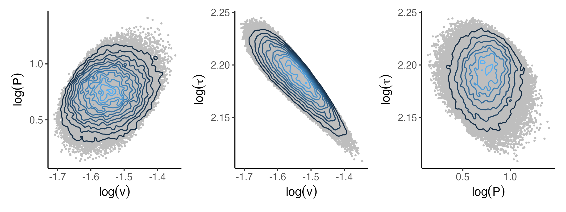
Figure 4 displays the marginal ABC posterior distributions produced by the OejMCMC, ejMCMC and DAMCMC algorithms. Figure 4 shows that the posterior of ejMCMC algorithm is consistent with that of OejMCMC algorithm. However, the posterior generated by the DAMCMC algorithm differs from that of OejMCMC and ejMCMC algorithms. Figure 5 shows the two-dimensional joint posterior distributions of the parameters obtained by using the ejMCMC algorithm. The posterior means and 95% credible intervals of provided by the OejMCMC, ejMCMC and DAMCMC algorithms are shown in Appendix Figure C.6. We also compute the correlation between posterior samples: , , . Recall that is the rate of increase of the blowfly population, is a resource limitation parameter set by the supply of food, and is the time delay that roughly equal to the time for an egg to grow up to a pupa. The positive correlation between and indicates that the blowfly population grows faster when there is a sufficient food supply. The tiny negative value of the correlation between and implies that the amount of food supply has a small impact on the period of being a pupa. The negative correlation between and indicates that the blowfly population will increase slower if the period for an egg to grow up to a pupa is longer.
6 Conclusion
We propose the early rejection ABC methods to accelerate parameter inference for complex statistical models. The main idea is to accurately reject parameter samples before generating synthetic data, and this is achieved by using a Gaussian process modeling to describe the relationship between the parameter and discrepancy. Our proposed method has two advantages compared with existing work. First, it utilizes MCMC moves for sampling parameters, which is more efficient in high-dimensional cases than sampling from a prior distribution. Second, it uses a pseudo Metropolis Hasting acceptance ratio to early reject samples in state space that are not worth exploring. The new method inherits the detailed balance condition and the posterior concentration property. It is also theoretically more efficient than the existing early rejection method.
We use several schemes to improve the performance of ejMCMC. To ensure the accuracy of the discrepancy model, we sequentially generate training points in areas with smaller discrepancy via a pilot run of ABC-SMC. We propose a prediction function for discrepancy model that balances accuracy and computational speed. An adaptive early rejection SMC is introduced by combining ABC-SMC and ejMCMC method. The ejASMC can adaptively select the sequence of thresholds and MCMC kernels, the particles are initialized via uniform design.
There are several lines of extensions and improvements for future work. We utilize identical kernel function and threshold value for and in the pseudo acceptance ratio (i.e. ) of ejMCMC. Using different kernel functions and threshold values can enhance the flexibility of algorithm. For example, decreasing the threshold of can decrease the rate of false positive. One future extension is to propose pseudo acceptance ratio with more general kernel functions. MCMC approaches often require a large number of simulations to make sure that the Markov chain converges to the stationary distribution. This limits their application to models that only a few hundreds simulations are possible. Compare to MCMC methods, importance sampling does not require to assess convergence and the consistency property holds under mild conditions. The efficiency of importance sampling methods mainly depends on proposal distributions. Our second line of future research is to combine GP-ABC and importance sampling approaches, by serving the fitted GP model as an efficient proposal distribution in importance sampling framework. In addition, we will investigate using the resulting importance sampling distribution to design efficient MCMC proposal distributions to improve the mixing of Markov chain. The current selection of discrepancy model is limited to models defined on Euclidean space. Lastly, we will extend to problems defined on more general space (e.g. a phylogenetic tree) in our future research.
Acknowledge
This work was supported by the National Natural Science Foundation of China (12131001 and 12101333), the startup fund of ShanghaiTech University, the Fundamental Research Funds for the Central Universities, LPMC, and KLMDASR. The authorship is listed in alphabetic order.
SUPPLEMENTAL MATERIALS
- Appendix A:
-
The proofs of all theoretical results presented in the main text.
- Appendix B:
-
Some description of algorithms not shown in the main text.
- Appendix C:
-
Some numerical results and some details of setups not shown in the main text.
References
- Åkesson et al. (2021) Åkesson, M., P. Singh, F. Wrede, and A. Hellander (2021). Convolutional neural networks as summary statistics for approximate bayesian computation. IEEE/ACM Transactions on Computational Biology and Bioinformatics 19(6), 3353–3365.
- Altman (1992) Altman, N. S. (1992). An introduction to kernel and nearest-neighbor nonparametric regression. The American Statistician 46(3), 175–185.
- Beaumont et al. (2002) Beaumont, M. A., W. Zhang, and D. J. Balding (2002, 12). Approximate Bayesian computation in population genetics. Genetics 162(4), 2025–2035.
- Berezansky et al. (2010) Berezansky, L., E. Braverman, and L. Idels (2010). Nicholson’s blowflies differential equations revisited: main results and open problems. Applied Mathematical Modelling 34(6), 1405–1417.
- Blum et al. (2013) Blum, M. G., M. A. Nunes, D. Prangle, and S. A. Sisson (2013). A comparative review of dimension reduction methods in approximate bayesian computation. Statistical Science 28(2), 189–208.
- Brooks et al. (2011) Brooks, S., A. Gelman, G. Jones, and X.-L. Meng (2011). Handbook of markov chain monte carlo, Chapter Likelihood-Free MCMC, pp. 313–333. New York: CRC press.
- Buchholz and Chopin (2019) Buchholz, A. and N. Chopin (2019). Improving approximate Bayesian computation via Quasi-Monte Carlo. Journal of Computational and Graphical Statistics 28(1), 205–219.
- Christen and Fox (2005) Christen, J. A. and C. Fox (2005). Markov chain monte carlo using an approximation. Journal of Computational and Graphical statistics 14(4), 795–810.
- Clarté et al. (2020) Clarté, G., C. P. Robert, R. J. Ryder, and J. Stoehr (2020, 11). Componentwise approximate Bayesian computation via Gibbs-like steps. Biometrika 108(3), 591–607.
- Cleveland and Devlin (1988) Cleveland, W. S. and S. J. Devlin (1988). Locally weighted regression: an approach to regression analysis by local fitting. Journal of the American statistical association 83(403), 596–610.
- Del Moral et al. (2006) Del Moral, P., A. Doucet, and A. Jasra (2006). Sequential Monte Carlo samplers. Journal of the Royal Statistical Society: Series B (Statistical Methodology) 68(3), 411–436.
- Del Moral et al. (2012) Del Moral, P., A. Doucet, and A. Jasra (2012). An adaptive sequential Monte Carlo method for approximate Bayesian computation. Statistics and Computing 22(5), 1009–1020.
- Doucet et al. (2001) Doucet, A., N. De Freitas, and N. Gordon (2001). An introduction to sequential Monte Carlo methods. In Sequential Monte Carlo methods in practice, pp. 3–14. Springer.
- Drovandi et al. (2018) Drovandi, C. C., M. T. Moores, and R. J. Boys (2018). Accelerating pseudo-marginal mcmc using gaussian processes. Computational Statistics & Data Analysis 118, 1–17.
- Epanechnikov (1969) Epanechnikov, V. A. (1969). Non-parametric estimation of a multivariate probability density. Theory of Probability & Its Applications 14(1), 153–158.
- Everitt and Rowińska (2021) Everitt, R. G. and P. A. Rowińska (2021). Delayed acceptance ABC-SMC. Journal of Computational and Graphical Statistics 30(1), 55–66.
- Fearnhead and Prangle (2012) Fearnhead, P. and D. Prangle (2012). Constructing summary statistics for approximate Bayesian computation: semi-automatic approximate Bayesian computation [with discussion]. Journal of the Royal Statistical Society. Series B (Statistical Methodology) 74(3), 419–474.
- Frazier et al. (2018) Frazier, D. T., G. M. Martin, C. P. Robert, and J. Rousseau (2018). Asymptotic properties of approximate bayesian computation. Biometrika 105(3), 593–607.
- Frazier et al. (2022) Frazier, D. T., D. J. Nott, C. Drovandi, and R. Kohn (2022). Bayesian inference using synthetic likelihood: Asymptotics and adjustments. Journal of the American Statistical Association 0(0), 1–12.
- Gelman et al. (1995) Gelman, A., J. B. Carlin, H. S. Stern, and D. B. Rubin (1995). Bayesian data analysis. Chapman and Hall/CRC.
- Golightly and Wilkinson (2010) Golightly, A. and D. Wilkinson (2010). Learning and Inference for Computational Systems Biology, Chapter Markov chain Monte Carlo algorithms for SDE parameter estimation, pp. 253–276. MIT Press.
- Gutmann and Corander (2016) Gutmann, M. U. and J. Corander (2016). Bayesian optimization for likelihood-free inference of simulator-based statistical models. Journal of Machine Learning Research 17(125), 1–47.
- Jiang et al. (2017) Jiang, B., T.-y. Wu, C. Zheng, and W. H. Wong (2017). Learning summary statistic for approximate bayesian computation via deep neural network. Statistica Sinica 27(4), 1595–1618.
- Joyce and Marjoram (2008) Joyce, P. and P. Marjoram (2008). Approximately sufficient statistics and bayesian computation. Statistical applications in genetics and molecular biology 7(1), Article 26.
- Järvenpää et al. (2019) Järvenpää, M., M. Gutmann, A. Vehtari, and P. Marttinen (2019, 06). Efficient acquisition rules for model-based approximate bayesian computation. Bayesian Analysis 14(2), 595–622.
- Järvenpää et al. (2018) Järvenpää, M., M. U. Gutmann, A. Vehtari, and P. Marttinen (2018). Gaussian process modelling in approximate Bayesian computation to estimate horizontal gene transfer in bacteria. The Annals of Applied Statistics 12(4), 2228 – 2251.
- Järvenpää et al. (2020) Järvenpää, M., A. Vehtari, and P. Marttinen (2020). Batch simulations and uncertainty quantification in gaussian process surrogate approximate bayesian computation. In Conference on Uncertainty in Artificial Intelligence, pp. 779–788. PMLR.
- Marin et al. (2012) Marin, J.-M., P. Pudlo, C. P. Robert, and R. J. Ryder (2012). Approximate bayesian computational methods. Statistics and Computing 22(6), 1167–1180.
- Marjoram et al. (2003) Marjoram, P., J. Molitor, V. Plagnol, and S. Tavaré (2003). Markov chain Monte Carlo without likelihoods. Proceedings of the National Academy of Sciences 100(26), 15324–15328.
- Maruyama (1955) Maruyama, G. (1955). Continuous markov processes and stochastic equations. Rendiconti del Circolo Matematico di Palermo 4, 48–90.
- May (1976) May, R. M. (1976). Models for single populations. In R. M. May (Ed.), Theoretical ecology, pp. 4–25. Philadelphia, Pennsylvania, USA: W. B. Saunders Company.
- Nicholson (1954) Nicholson, A. J. (1954). An outline of the dynamics of animal populations. Australian Journal of Zoology 2(1), 9–65.
- Nunes and Balding (2010) Nunes, M. A. and D. J. Balding (2010). On optimal selection of summary statistics for approximate bayesian computation. Statistical applications in genetics and molecular biology 9(1), 34.
- Picchini (2014) Picchini, U. (2014). Inference for SDE models via approximate Bayesian computation. Journal of Computational and Graphical Statistics 23(4), 1080–1100.
- Price et al. (2017) Price, L. F., C. C. Drovandi, A. Lee, and D. J. Nott (2017, jul). Bayesian synthetic likelihood. Journal of Computational and Graphical Statistics 27(1), 1–11.
- Pritchard et al. (1999) Pritchard, J. K., M. T. Seielstad, A. Perez-Lezaun, and M. W. Feldman (1999, 12). Population growth of human Y chromosomes: a study of Y chromosome microsatellites. Molecular Biology and Evolution 16(12), 1791–1798.
- Pudlo et al. (2016) Pudlo, P., J.-M. Marin, A. Estoup, J.-M. Cornuet, M. Gautier, and C. P. Robert (2016). Reliable abc model choice via random forests. Bioinformatics 32(6), 859–866.
- Sisson and Fan (2010) Sisson, S. A. and Y. Fan (2010). Likelihood-free markov chain monte carlo. In S. Brooks, G. L. Jones, and X.-L. Meng (Eds.), Handbook of Markov Chain Monte Carlo. Chapman and Hall/CRC Press. In press.
- Sisson et al. (2018) Sisson, S. A., Y. Fan, and M. Beaumont (2018). Handbook of approximate Bayesian computation. CRC Press.
- Sisson et al. (2007) Sisson, S. A., Y. Fan, and M. M. Tanaka (2007). Sequential Monte Carlo without likelihoods. Proceedings of the National Academy of Sciences 104(6), 1760–1765.
- Soetaert et al. (2010) Soetaert, K., T. Petzoldt, and R. W. Setzer (2010). Solving differential equations in r: package desolve. Journal of statistical software 33, 1–25.
- Stanton et al. (2021) Stanton, S., W. Maddox, I. Delbridge, and A. G. Wilson (2021). Kernel interpolation for scalable online gaussian processes. In International Conference on Artificial Intelligence and Statistics, pp. 3133–3141. PMLR.
- Wegmann et al. (2009) Wegmann, D., C. Leuenberger, and L. Excoffier (2009, 08). Efficient approximate Bayesian computation coupled with Markov chain Monte Carlo without likelihood. Genetics 182(4), 1207–1218.
- Wilkinson (2014) Wilkinson, R. (2014). Accelerating abc methods using gaussian processes. In Artificial Intelligence and Statistics, pp. 1015–1023. PMLR.