Urban mapping in Dar es Salaam using AJIVE

The phone call detail record (CDR) data were collected from $n_{T}=593$ base transceiver station (BTS) towers located over Dar es Salaam (shown in Figure 2), during 122 days in 2014¹¹1For more details, see Engelmann et al., (2018).. For each tower, information was collected about all call and SMS interactions recorded, including the time of the interaction, and the user IDs of both sender and receiver. This information was used to calculate a set of features for each user, such as the number of calls and SMS sent and received, the number of BTS towers visited, and the mean time between interactions; Table 2 in the supplementary material gives the full list of features. There are also 5 features calculated at tower level (such as the total number of interactions recorded by each tower). To convert user-level features to tower features, each user ID was assigned a “home” tower based on where the majority of their night-time interactions (between 10pm and 6am) took place; the tower features were calculated as the mean values across individuals who were assigned to that tower.

To calculate feature vectors for each subward, it was first necessary to determine the areas of overlap between the subwards and the regions served by each tower. The tower regions were calculated by constructing a Voronoi diagram, in which a polygon is placed around each tower in such a way that any point contained within it is closer to that tower than to any other. We refer to these polygons as the tower regions. The subward feature vectors were then calculated as weighted averages over the tower feature vectors, with weights proportional to the areas of overlap between the tower regions and subwards.

To describe this mathematically, we label the subwards $S_{1},\ldots,S_{n}$, and the tower regions $T_{1},\ldots,T_{n_{T}}$. Let $\boldsymbol{\Gamma}$ denote an $n\times n_{T}$ matrix with entries $\gamma_{ij}$, where

Then the feature vector corresponding to subward $S_{i}$ is given by

where $\boldsymbol{\gamma}_{1},\ldots,\boldsymbol{\gamma}_{n}$ are the row vectors of $\boldsymbol{\Gamma}$, and $\boldsymbol{1}$ is an $n_{T}\times 1$ vector with all elements equal to 1. After calculating the matrix of subward CDR features $\boldsymbol{X}_{1}$, each column is $98\%$ winsorized (i.e. the largest and smallest 1% are replaced with the values of the 99th and 1st percentiles) to remove the effect of large outliers, and then standardized so that each feature has mean 0 and variance 1 across subwards.

The image data consists of high-resolution, georeferenced satellite imagery of Dar es Salaam, which is made available by MAXAR (at https://www.maxar.com/open-data/covid19). We divided the images into subwards to create an image for each subward, discarding any sections that were covered by cloud. As a result, we have full or partial images for 383 subwards; the remaining 69 had to be excluded from the analysis, due to either being outside the area covered by the satellite imagery, or to the corresponding section of the image being entirely obscured by cloud. Figure 3 shows an example of the image data for a particular subward.

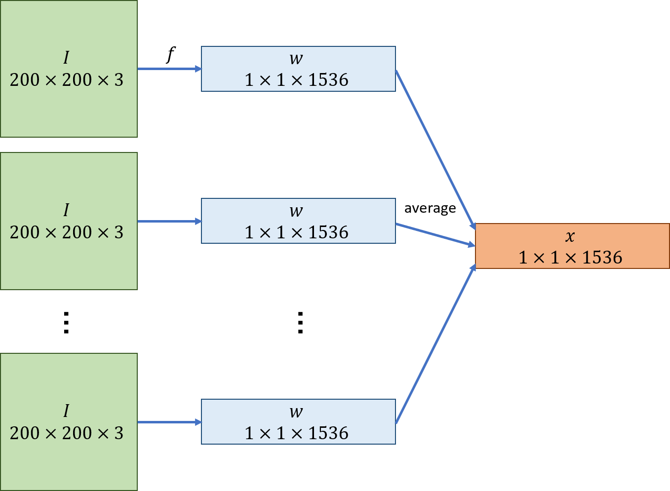
The subward images are high-dimensional and are of different sizes and shapes. To apply AJIVE or PCA, we need to construct a matrix representation of the data, where a row vector corresponds to each subward. To do this, we follow Carmichael et al., (2021) by randomly sampling a set of uniformly-sized patches from each subward image, and applying a pre-trained convolutional neural network (CNN) to map each patch to a lower-dimensional vector. We then take the mean feature vector across the patches for each subward. Figure 4 illustrates this process.

For each subward, we took 10 patches of dimension $200\times 200$ pixels, sampling the top-left pixel uniformly from all possible locations (i.e. the image with the 199 right-most and bottom-most pixels excluded). Patches could overlap. Any patches containing more than $1\%$ black background pixels were replaced, to ensure that the image backgrounds were not a prominent feature in the patches.

For the CNN, we used InceptionResNet-V2 Szegedy et al., (2016) trained on ImageNet; this is one of the best-performing models on ImageNet. The schema is given in Figure 15 of Szegedy et al., (2016). A CNN takes as its input a $d_{1}\times d_{2}\times d_{3}$ dimensional array of pixel values (where $d_{1}\times d_{2}$ are the dimensions of the image, and $d_{3}$ is the number of colour channels, in our case 3), where each element has an integer value between 0 and 255, and outputs a $v_{1}\times v_{2}\times v_{3}$ dimensional feature array, where $v_{1}v_{2}v_{3}<<d_{1}d_{2}d_{3}$. If we let $\mathcal{I}$ denote the space of possible images, the CNN can be defined as a mapping

The values of $v_{1}$, $v_{2}$, and $v_{3}$ are determined by the model architecture. This array is then usually fed into a final classification layer, which converts it into a vector; however, as the classification task the model was trained on is not directly relevant to our situation, we did not use this. Given the input patch dimensions and choice of model architecture, the output we obtain for each patch is a $4\times 4\times 1536$ dimensional array. To reduce the dimension of this further, we used maxpooling, taking the maximum value in each $4\times 4\times 1$ dimensional sub-array to produce a 1536-dimensional vector. We then took the mean across patches to generate a feature vector for each subward. As with the CDR features, the image features are then $98\%$ winsorized and standardized to have mean 0 and variance 1.

The survey data were collected in two phases in May and August 2019. In each subward, data were collected from approximately 8 respondents who were asked to answer questions on that subward. Most subwards had 8 respondents, although some had more or fewer; all had between 2 and 17.

The questions cover various aspects such as poverty and unemployment, education, and medical facilities. The data were originally collected (Ellis,, 2021) to create a set of fine-grained, socio-demographic data about Dar es Salaam, which could be used to inform research on topics such as deprivation and forced labour risk, and to provide a ground truth against which models could be compared. Not all of the questions and responses could be used in our analysis, as some questions had categorical or write-in answers: we only included questions which had numerical or ordinal responses. Tables 3 and 4 in the supplementary material give the full list of survey questions in the data set used for this paper, and possible responses. For each subward we take the median responses for the respondents. The variables are then centred and scaled so that each response variable has mean 0 and variance 1.

Figures 5 and 6 show pairwise correlations between each of the CDR, image, and survey features. In each case there are several clusters of correlated variables, which suggests that dimension reduction should be useful.

Our aim is to explore how we can use the CDR and image data to map deprivation. To provide a comparison, we use deprivation estimates for Dar es Salaam calculated from comparative judgment data, using the Bayesian Spatial Bradley-Terry model (Seymour et al.,, 2022). These are available in the R package BSBT and consist of a score between -1.2 and 2.2 for each subward in Dar es Salaam, where higher scores indicate less deprived subwards. Figure 7 shows a plot of these deprivation scores for the subwards that are included in our analysis.

For a centred $n\times p$ data matrix, $\boldsymbol{X}$, PCA identifies the subspace of a chosen dimension, $r$, in which the data have greatest variance. It can be computed in terms of the Singular Value Decomposition (SVD):

where, with $m=\min\{n,p\}$, $\boldsymbol{\Sigma}$ is an $m\times m$ diagonal matrix containing the $m$ singular values of $\boldsymbol{X}$ in decreasing order; and $\boldsymbol{U}$ and $\boldsymbol{V}$ are respectively $n\times m$ and $p\times m$ matrices with columns corresponding respectively to the left and right singular vectors of $\boldsymbol{X}$, such that $\boldsymbol{U}^{\top}\boldsymbol{U}=\boldsymbol{V}^{\top}\boldsymbol{V}=\boldsymbol{I}_{m}$ (the $m\times m$ identity matrix).

Reducing the dimension of the data to the chosen dimension $r$ $(<m)$ by PCA entails approximating $\boldsymbol{X}$ using the rank-$r$ truncated SVD, that is

where $\boldsymbol{U}_{r}$ and $\boldsymbol{V}_{r}$ are matrices containing the first $r$ columns of $\boldsymbol{U}$ and $\boldsymbol{V}$ respectively, and $\boldsymbol{\Sigma}_{r}$ is the $r\times r$ diagonal matrix containing the first $r$ singular values of $\boldsymbol{X}$. The PC scores are the rows of the $n\times r$ matrix $\boldsymbol{V}_{r}$.

Angle-Based Joint and Individual Variation Explained (AJIVE) (Feng et al.,, 2018) is a dimension reduction algorithm which can be applied to two or more data sets, where the data correspond to the same group of individuals, but are of different types. It is applicable when we believe there is some joint structure common to both data sets, but also some information which is unique to each: in contrast to methods such as Principal Component Analysis, where each data matrix is decomposed separately, or Canonical Correlation Analysis, which finds only joint components, AJIVE allows us to analyse both joint and individual variation within the data. It was developed as a more efficient version of Joint and Individual Variation Explained (JIVE) (Lock et al.,, 2013).

AJIVE (Feng et al.,, 2018) aims to decompose each data matrix $\boldsymbol{X}_{i}$ as

where $\boldsymbol{J}=\left(\boldsymbol{J}_{1}~{}\cdots~{}\boldsymbol{J}_{k}\right)$ is the joint variation matrix (of rank $r_{J}$), $\boldsymbol{A}_{1},\ldots,\boldsymbol{A}_{k}$ are the individual variation matrices (each of which have rank $r_{i}$), and $\boldsymbol{E}_{1},\ldots,\boldsymbol{E}_{k}$ represent noise.

We can decompose $\boldsymbol{J}$ as

which we obtain by taking the (exact) rank-$r_{J}$ SVD of $\boldsymbol{J}$. $\boldsymbol{U}_{J}$ is the $n\times r_{J}$ matrix of joint scores (in our case, each row corresponds to a subward), and $\boldsymbol{V}_{J}$ is the $p\times r_{J}$ matrix of joint loadings (each row corresponds to a CDR or image feature). $\boldsymbol{\Sigma}_{J}$ contains the singular values of $\boldsymbol{J}$ and controls the relative weights of each component. Figure 8 illustrates this decomposition.

Similarly, for the $i$th individual component ($i=1,\ldots,k$) we decompose $\boldsymbol{A}_{i}$ as

where $\boldsymbol{U}_{i}$ is the $n\times r_{i}$ score matrix, $\boldsymbol{V}_{i}$ the $p_{i}\times r_{i}$ loading matrix, and $\boldsymbol{\Sigma}_{i}$ contains the $r_{i}$ non-zero singular values of $\boldsymbol{A}_{i}$.

The AJIVE algorithm is given in detail in (Feng et al.,, 2018); we give an outline here. The algorithm has three main stages:

Stage 1. We choose initial signal ranks $\tilde{r}_{1},\ldots,\tilde{r}_{k}$ (see Section 3.3) and approximate each $\boldsymbol{X}_{i}$ by its rank-$\tilde{r}_{i}$ truncated SVD:

Stage 2. To estimate the joint scores $\boldsymbol{U}_{J}$, we combine the score matrices into one matrix $\boldsymbol{M}$, from which we will extract the joint signal:

and calculate its SVD:

We then choose the joint rank $r_{J}$, based on the singular values of $\boldsymbol{M}$, (again, see Section 3.3), and set the estimate of the joint scores to be $\tilde{\boldsymbol{U}}_{J}=\tilde{\boldsymbol{U}}_{M}$, where $\tilde{\boldsymbol{U}}_{M}$ is a matrix containing the first $r_{J}$ columns of $\boldsymbol{U}_{M}$.

To estimate the joint matrix $\boldsymbol{J}$, we project $\boldsymbol{X}=\left(\boldsymbol{X}_{1},\boldsymbol{X}_{2}\right)$ onto $\tilde{\boldsymbol{U}}_{J}$:

and decompose $\hat{\boldsymbol{J}}$ as $\hat{\boldsymbol{J}}=\hat{\boldsymbol{U}}_{J}\hat{\boldsymbol{\Sigma}}_{J}\hat{\boldsymbol{V}}_{J}^{\top}$, by taking its rank-$r_{J}$ SVD (which gives an exact decomposition since $\hat{\boldsymbol{J}}$ has rank $r_{J}$):

(Note that although generally $\tilde{\boldsymbol{U}}_{J}\neq\hat{\boldsymbol{U}}_{J}$ (unless $r_{J}=1$), we have $\tilde{\boldsymbol{U}}_{J}\tilde{\boldsymbol{U}}_{J}^{\top}=\hat{\boldsymbol{U}}_{J}\hat{\boldsymbol{U}}_{J}^{\top}$: they are both estimates of the score space of $\hat{\boldsymbol{J}}$.)

Stage 3. To estimate the individual matrices $\boldsymbol{A}_{i}$, we note that for each $i$, we require the joint scores $\boldsymbol{U}_{i}$ to be orthogonal to $\hat{\boldsymbol{U}}_{J}$. Hence, we project each $\boldsymbol{X}_{i}$ onto the orthogonal complement of $\hat{\boldsymbol{J}}$:

where $\boldsymbol{I}_{n}$ is the $n\times n$ identity matrix. We then take a final rank-$r_{i}$ SVD of this matrix $\tilde{\boldsymbol{X}}_{i}$:

To implement AJIVE we must provide estimates of the initial ranks $\tilde{r}_{1},\ldots,\tilde{r}_{k}$, joint rank $r_{J}$, and individual ranks $r_{1},\ldots,r_{k}$. We describe here how we do this. For simplicity, we will refer to the case where we have the CDR and image data, so $k=2$: we later incorporate the survey data as well, but the methods are the same.

Initial ranks. In selecting the initial ranks, we aim to distinguish signal from noise in each data set. We do this by inspecting scree plots of $\boldsymbol{X}_{1}$ and $\boldsymbol{X}_{2}$ (Figure 9 (a)–(b)). On both plots there is a sizeable jump after the third singular value, so we take $\tilde{r}_{1}=\tilde{r}_{2}=3$.

Joint rank. After combining the initial score matrices into one matrix $\boldsymbol{M}$ (see previous section), we want to find out which components of $\boldsymbol{M}$ have sufficiently large singular values to be regarded as part of the joint signal. To do this we use a random direction bound, as in Feng et al., (2018). To recap, we have

where $\boldsymbol{M}$ is an $n\times\left(\tilde{r}_{1}+\tilde{r}_{2}\right)$ dimensional matrix.

We create 1000 random matrices of the same dimensions as $\boldsymbol{M}$, with elements sampled independently from $U(0,1)$, and calculate the largest singular value in each case. We take the 95th percentile of these values as a lower bound for the singular values of $\boldsymbol{M}$ that correspond to joint signal. Figure 9 (c) illustrates this process for the CDR and image data. The red points show the ordered singular values of $\boldsymbol{M}$ (excluding those that are equal to 0), whilst the black points correspond to the maximum singular values of each randomly generated matrix, as described above. The horizontal black line corresponds to the threshold for the joint signal. There are two red points above the black line, so we take $r_{J}=2$.

Individual ranks. After calculating the joint components, we subtract from each $\boldsymbol{X}_{i}$ the corresponding part of the joint signal matrix, and calculate its SVD:

The initial rank $\tilde{r}_{i}$ was selected by inspecting a scree plot, but we could equivalently have selected a threshold

where $\lambda_{\tilde{r}_{i}}^{i}$ and $\lambda_{\tilde{r}_{i}+1}^{i}$ are the $\tilde{r}_{i}$th and $\tilde{r}_{i}+1$th largest singular values of $\boldsymbol{X}_{i}$, such that we only keep components with singular values greater than or equal to $\nu_{i}$. For the individual components, we use the same threshold, so we keep the individual components which have corresponding singular values greater than or equal to $\nu_{i}$ and discard those which are smaller. For the CDR and image data, this gives $r_{1}=r_{2}=1$.

Figure 10 shows the results for the first joint component (JC1). The positive end of the component shows green, rural areas; at the negative end, the patches show built-up areas with small, residential buildings. We can also see from Figure 10(a) that most subwards with negative scores are small and located close to the city centre. The most positive CDR features are the number of calls initiated by users, the average distance between users and the people they call, and the ratio of calls to SMS. This suggests that residents in these areas are more likely to initiate calls and to make calls rather than sending SMS, compared to those at the negative end of the component. It also seems reasonable that people living in rural areas, with low population density, would tend to communicate with people further away, as there are fewer people living close by. The most negative CDR features are the number of day, evening, and night interactions, and the number of active users; these are likely to be correlated with population.

For the second joint component (JC2) (Figure 11), the subwards with the most positive scores again appear to be more rural areas, but the negative end appears to show mostly commercial and industrial areas. The most negative subwards are located close to the city centre and on the coast, whilst the subwards in the south-west and south-east of the city tend to be those with the most positive scores. The most positive CDR features are the percentage of contacts that account for $80\%$ of a user’s call interactions, entropy of contacts — which are both measures of the diversity of contacts with whom a user interacts — and the number of active users. Looking at the CDR features with the most negative loadings, we infer that at this end of the component, users move around more (to different towers), make more calls, and use their phones on more days.

For the CDR individual component (IC1^CDR) (Figure 12), the most positive CDR features are those related to entropy of locations and contacts, and the total number of SMS sent. At the negative end are the ratio of calls to texts, and the standard deviation of interevent times. This end of the component also seems to contain built-up areas with taller buildings, although it is less clear what the patches from the positive end show. (This is perhaps not surprising, as this component does not directly use information from the patches.)

The most positive subward seems to have a particularly extreme value: we can see that it is much brighter than all the other subwards in Figure 12 (a). This subward contains the University of Dar es Salaam, as well as a large shopping centre (part of the roof of this is shown in one of the patches in Figure 12 (c)); it seems reasonable to assume that these would have an impact on patterns of phone usage, as people’s activities in this subward will likely be different to other areas of the city.

For the image individual component (IC1^Image) (Figure 13), it looks like the positive end corresponds to industrial and commercial areas, whereas the negative end is mostly rural. There are no CDR feature loadings to display for this component. As for IC1^CDR, there appears to be one extreme subward, this time at the negative end of the component: one of the patches from this component (Figure 13 (b)) looks unusual, so this may be responsible. However, when we re-implement AJIVE with this subward removed, there is not a noticeable difference in the results for the other subwards, so it does not seem to be having too much influence on the results. (This is also the case for the outlier subward in IC1^CDR.

IC1^CDR and IC1^Image have virtually no correlation ($\rho=0.03$), so we can surmise that all joint variation is adequately captured by JC1 and JC2: correlation between the individual components would suggest that the joint rank was too small. We can therefore assume that the information captured in IC1^CDR and IC1^Image is unique to the CDR and image data sets respectively.

Table 1 briefly summarises our observations in this section.

One of the main aims of this paper is to investigate whether AJIVE can be used to predict deprivation. We are interested in whether our methods and data sources can be used to do this in situations where alternative data sources are unavailable; however, to assess how well it works, we here use deprivation estimates created from a completely distinct data set (details were given in Section 2.4).

Figure 15 shows correlations between the deprivation estimates and AJIVE and PC scores. There is a fairly strong positive correlation between deprivation and JC2 ($\rho=0.67$). Hence, this component seems to be picking up joint variation in the data which is relevant for determining deprivation. In particular, this indicates that deprivation information is present in both $\boldsymbol{X}_{1}$ and $\boldsymbol{X}_{2}$. For each of the other AJIVE components there is no or very little correlation with deprivation.

One question is whether using AJIVE gives a significant advantage over using Principal Components Analysis (PCA). PCA can be used either on $\boldsymbol{X}_{1}$ and $\boldsymbol{X}_{2}$ separately, or on the concatenated data matrix $\boldsymbol{X}=\left(\boldsymbol{X}_{1},\boldsymbol{X}_{2}\right)$. We consider both of these options here, and compare their output to that of AJIVE.

As a reminder, from Section 3.1, using rank-$r$ PCA we represent an $n\times p$ data matrix $\boldsymbol{X}$ as

where $\boldsymbol{U}_{r}$ and $\boldsymbol{V}_{r}$ are $n\times r$ and $p\times r$ matrices containing the first $r$ left and right singular vectors of $\boldsymbol{X}$ respectively, and $\boldsymbol{\Sigma}_{r}$ is an $r\times r$ diagonal matrix containing the first $r$ singular values of $\boldsymbol{X}$ along its diagonal. As with AJIVE, we can interpret the columns of $\boldsymbol{U}_{r}$ and $\boldsymbol{V}_{r}$ as score and loading vectors respectively. The singular values in $\boldsymbol{\Sigma}_{r}$ control the relative importance of each component.

To compare AJIVE with separate PC analyses of $\boldsymbol{X}_{1}$ and $\boldsymbol{X}_{2}$, we computed the first three principal components (referred to as PC1, PC2, and PC3) for each data set. (Each data set has three AJIVE components related to it — two joint and one individual — so this seems a fair comparison.) Figure 15 shows correlations between scores for the AJIVE and PC components. (Note that JC1 and JC2 are forced to be orthogonal to each other, as well as to the individual components, and the PC components for each data matrix are also forced to be orthogonal.)

We see that JC1 is strongly correlated with PC2^CDR and is also correlated with both PC1^Image and PC2^Image, whilst JC2 is correlated with PC1^CDR and PC3^Image. IC1^CDR is strongly correlated with PC3^CDR, and IC1^Image is correlated with PC1^Image and PC2^Image. IC1^CDR appears to be uncorrelated with the image PC scores, and the same applies to IC1^Image and the CDR PC scores. AJIVE appears to give similar overall results to doing separate PCAs of the CDR and image data, but the division of components is different. Hence, AJIVE identifies which parts of the components are common to both data sets and which are unique to each data set.

When doing PCA on the concatenated data matrix $\boldsymbol{X}=\left(\boldsymbol{X}_{1}\hskip 2.84544pt\boldsymbol{X}_{2}\right)$, we find that the first few PCs of $\boldsymbol{X}$ are almost identical to the corresponding PCs of $\boldsymbol{X}_{2}$. This is not surprising as $\boldsymbol{X}_{2}$ has a much higher dimensionality than $\boldsymbol{X}_{1}$ ($p_{1}=20,p_{2}=1536$). However, this shows that applying PCA to the concatenated data matrix $\boldsymbol{X}$ is not useful for our data, as we essentially lose the information from $\boldsymbol{X}_{1}$. This would also apply to other situations where the number of dimensions differs greatly between data matrices.

So far, we have looked at applying AJIVE and PCA to the CDR and image data sets. We now repeat the foregoing analysis but with the addition of the survey data introduced earlier in Section 2.3. Recall that the survey data are slower and more costly to collect than the CDR and image data, so it is natural to ask: what extra information does the survey data provide, and does it warrant the cost of collecting the data in the first place?

The scree plot (Figure 17) suggests an initial rank of 2 for the survey data. Applying the random direction bound to estimate the joint rank (as in Section 3.3, but using all three data matrices) returns a joint rank $r_{J}=2$. We also obtain individual rank estimates of $r_{1}=r_{2}=r_{3}=1$.

Figure 18 shows a plot of the survey individual component (IC1^Survey) scores for each subward, and 5 patches from two most positive and most negative subwards. Corresponding plots for the other components (JC1, JC2, IC1^CDR, and IC1^Image) are shown in the supplementary material (Section C): they are very similar to those we obtained using only the CDR and image data (Figures 10 to 13). Figure 19 shows correlations between AJIVE and PC components for the three data matrices. Comparing with Figure 15, the relations between JC1, JC2, IC1^CDR and IC1^Image, and the CDR and image PCs are virtually unchanged, so incorporating the survey data does not have much effect on the decomposition. However, looking at the survey individual component allows us to see what information may be present in the survey data that we cannot get from the other data sets. From Figure 18 (b), it appears that IC1^Survey highlights a risk of forced labour and exploitation: the variables with the most negative loadings are those relating to forced work and arranged marriage, whilst as the positive end we have higher rates of children and teenagers in education, and more use of technology, which may be associated with lower risks of forced labour.

We have investigated correlation between the dimension-reduced representations of the data (AJIVE and PC scores) and deprivation scores, but the approaches to dimension reduction were “unsupervised” in the sense that they did not involve using the deprivation data. In this section, we consider the “supervised” approach of using deprivation as a response variable in a regression model geared towards prediction of deprivation from the CDR, image and survey data. We particularly investigate whether it aids prediction to use AJIVE and/or PCA as a step of dimension reduction to construct “features” for the regression model.

A recently introduced approach (Ding et al.,, 2022) for incorporating multiple data “views” into a regression model involves minimising the objective

with respect to the regression parameters $\boldsymbol{\beta}_{1},\ldots,\boldsymbol{\beta}_{M}$, in which $\boldsymbol{\beta}_{m}$ is $p_{m}\times 1$ vector of parameters corresponding to the $m$th view, $\boldsymbol{Z}_{m}$, and $\mathbf{y}$ is a response variable to be predicted. For the special case with parameters $\rho=0$ and $\lambda_{1}=\cdots=\lambda_{m}$, this is the objective for LASSO regression of $\mathbf{y}$ on the concatenated data $\boldsymbol{Z}=(\boldsymbol{Z}_{1},\ldots,\boldsymbol{Z}_{M})$. But when $\rho>0$, the final term encourages “cooperation” between the predictions from the different individual views, which in some circumstances leads to better predictive performance for out-of-sample data, i.e. new observations not used in fitting the model (Ding et al.,, 2022).

For a given choice of $\rho,\lambda_{1},\ldots,\lambda_{M}$, the fitted parameters $\hat{\boldsymbol{\beta}}=(\hat{\boldsymbol{\beta}}_{1}^{\top},\ldots,\hat{\boldsymbol{\beta}}_{M}^{\top})^{\top}$ are determined by minimising (3), and prediction of the response variable for a new observation with predictor vector $\mathbf{z}=(\mathbf{z}_{1}^{\top},\ldots,\mathbf{z}_{M}^{\top})^{\top}$ is $\hat{\boldsymbol{y}}=\mathbf{z}^{\top}\hat{\boldsymbol{\beta}}$. One way to select the hyper-parameters $\rho,\lambda_{1},\ldots,\lambda_{M}$ is by cross-validation, i.e., repeatedly partitioning the observations into training and “held-out” test sets, finding $\hat{\boldsymbol{\beta}}$ based on the training data for various different values of the hyper-parameters, then selecting the hyper-parameter values that minimise mean-squared error in predictions for the held-out test data.

To compare the performance of different $\boldsymbol{Z}$’s, we select $\lambda_{1},\ldots,\lambda_{M}$ using cross-validation with 20 folds, and calculate the average Mean Squared Error (MSE) across folds: we choose the value of $\boldsymbol{\lambda}$ which minimizes this. A lower MSE means the model is more accurate at predicting deprivation $\boldsymbol{y}$. In various numerical investigations exploring values $\rho\geq 0$ with different choices of predictor data $\boldsymbol{Z}$, we found no circumstances where $\rho>0$ performed better than $\rho=0$ — see for example Figure 20 — so we set $\rho=0$ in all following experiments.

Figure 21 shows the results using $\rho=0$ and different choices for $\boldsymbol{Z}$. Except for PCA on the CDR data (where we have a maximum of 20 components to work with), all AJIVE and PCA regressions are done with 30 total components, which are divided equally between data sets and, for AJIVE, between joint and individual components.

We first consider using each data set individually, setting $\boldsymbol{Z}$ to be either the entire data set or the matrix of principal components. The CDR data gives the lowest MSE, whilst the survey data does by far the worst. In each case using PCA gives similar results to using the entire data set.

We then combine data sets: we consider using the CDR and image data, as we did for our main analysis, and then adding in the survey data. Here, we find that PCA regression does slightly better than using the entire data. The difference between PCA and AJIVE is less clear: when we have just the CDR and image data, AJIVE seems to do slightly better than PCA, but this is not the case once we also add in the survey data, although the differences in MSE are very small, so it is difficult to draw firm conclusions. However, as mentioned above AJIVE with CDR, image and survey data gives the additional useful information about forced labour risk and so this is our preferred approach.

Figure 22 shows a plot of the MSE versus the number of components, when we use several combinations of components for the CDR and image data. The black horizontal line corresponds to the null model. In each case the MSE decreases until we have around 20 components, then levels off. There does not appear to be much difference in performance between the three choices of $\boldsymbol{Z}$ we use here.

References

- Babenko et al., (2017) Babenko, B., Hersh, J., Newhouse, D., Ramakrishnan, A., and Swartz, T. (2017). Poverty mapping using convolutional neural networks trained on high and medium resolution satellite images, with an application in Mexico. arXiv preprint arXiv:1711.06323.
- Blumenstock et al., (2015) Blumenstock, J., Cadamuro, G., and On, R. (2015). Predicting poverty and wealth from mobile phone metadata. Science, 350(6264):1073–1076.
- Carmichael et al., (2021) Carmichael, I., Calhoun, B. C., Hoadley, K. A., Troester, M. A., Geradts, J., Couture, H. D., Olsson, L., Perou, C. M., Niethammer, M., Hannig, J., and Marron, J. S. (2021). Joint and individual analysis of breast cancer histologic images and genomic covariates. The Annals of Applied Statistics, 15(4):1697.
- Ding et al., (2022) Ding, D. Y., Li, S., Narasimhan, B., and Tibshirani, R. (2022). Cooperative learning for multiview analysis. Proceedings of the National Academy of Sciences, 119(38):e2202113119.
- Ellis, (2021) Ellis, M. (2021). Detection of vulnerable communities in East Africa via novel data streams and dynamic stochastic block models. PhD thesis, University of Nottingham.
- Engelmann et al., (2018) Engelmann, G., Smith, G., and Goulding, J. (2018). The unbanked and poverty: Predicting area-level socio-economic vulnerability from M-Money transactions. In 2018 IEEE International Conference on Big Data, pages 1357–1366. IEEE.
- Engstrom et al., (2017) Engstrom, R., Hersh, J. S., and Newhouse, D. L. (2017). Poverty from space: Using high-resolution satellite imagery for estimating economic well-being. World Bank Policy Research Working Paper, 8284.
- Feng et al., (2018) Feng, Q., Jiang, M., Hannig, J., and Marron, J. (2018). Angle-based joint and individual variation explained. Journal of multivariate analysis, 166:241–265.
- Lock et al., (2013) Lock, E. F., Hoadley, K. A., Marron, J. S., and Nobel, A. B. (2013). Joint and individual variation explained (JIVE) for integrated analysis of multiple data types. The annals of applied statistics, 7(1):523.
- Locke and Henley, (2016) Locke, A. and Henley, G. (2016). Urbanisation, land and property rights.
- Seymour et al., (2022) Seymour, R. G., Sirl, D., Preston, S. P., Dryden, I. L., Ellis, M. J. A., Perrat, B., and Goulding, J. (2022). The Bayesian Spatial Bradley–Terry model: Urban deprivation modelling in Tanzania. Journal of the Royal Statistical Society: Series C (Applied Statistics), 71(2):288–308.
- Shannon, (1948) Shannon, C. E. (1948). A mathematical theory of communication. The Bell system technical journal, 27(3):379–423.
- Smith et al., (2013) Smith, C., Mashhadi, A., and Capra, L. (2013). Ubiquitous sensing for mapping poverty in developing countries. Paper submitted to the Orange D4D Challenge.
- Smith-Clarke et al., (2014) Smith-Clarke, C., Mashhadi, A., and Capra, L. (2014). Poverty on the cheap: Estimating poverty maps using aggregated mobile communication networks. In Proceedings of the SIGCHI conference on human factors in computing systems, pages 511–520.
- Steele et al., (2017) Steele, J. E., Sundsøy, P. R., Pezzulo, C., Alegana, V. A., Bird, T. J., Blumenstock, J., Bjelland, J., Engø-Monsen, K., de Montjoye, Y.-A., Iqbal, A. M., Hadiuzzaman, K. N., Lu, X., Wetter, E., Tatem, A. J., and Bengtsson, L. (2017). Mapping poverty using mobile phone and satellite data. Journal of The Royal Society Interface, 14(127):20160690.
- Szegedy et al., (2016) Szegedy, C., Ioffe, S., Vanhoucke, V., and Alemi, A. (2016). Inception-v4, Inception-ResNet and the impact of residual connections on learning. In Proceedings of the Thirty-First AAAI Conference on Artificial Intelligence.
- Xie et al., (2016) Xie, M., Jean, N., Burke, M., Lobell, D., and Ermon, S. (2016). Transfer learning from deep features for remote sensing and poverty mapping. In Proceedings of the Thirtieth AAAI Conference on Artifical Intelligence (AAAI-16), pages 3929–3935.
Supplementary material
Appendix A List of CDR features