10.7155/jgaa.00587 \Issue2611711982022 \HeadingAuthorKlawitter and Mchedlidze \HeadingTitleUpward planar drawings with two slopes \authorOrcid[first]Jonathan [email protected] first]University of Würzburg, Germany \authorOrcid[second]Tamara [email protected] second]Utrecht University, The Netherlands \submittedNovember 2021\reviewedMarch 2021\finalMay 2021\publishedJune 2021\typeRegular paper\editorG. Liotta
Upward planar drawings with two slopes
Abstract
In an upward planar 2-slope drawing of a digraph, edges are drawn as straight-line segments in the upward direction without crossings using only two different slopes. We investigate whether a given upward planar digraph admits such a drawing and, if so, how to construct it. For the fixed embedding scenario, we give a simple characterisation and a linear-time construction by adopting algorithms from orthogonal drawings. For the variable embedding scenario, we describe a linear-time algorithm for single-source digraphs, a quartic-time algorithm for series-parallel digraphs, and a fixed-parameter tractable algorithm for general digraphs. For the latter two classes, we make use of SPQR-trees and the notion of upward spirality. As an application of this drawing style, we show how to draw an upward planar phylogenetic network with two slopes such that all leaves lie on a horizontal line.
1 Introduction
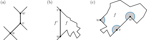
When we visualize directed graphs (digraphs for short) that model hierarchical relations with node-link diagrams, we traditionally turn edge directions into geometric directions by letting each edge point upward. Aiming for visual clarity, we would like such an upward drawing to be planar, that is, no two edges should cross [14]. If this is possible, the resulting drawing is called upward planar drawing; see Figure 1 (a). Interestingly, as Di Battista and Tamassia [15] have shown, every upward planar drawing can be turned into one where each edge is drawn with a single line segment; such a straight-line drawing may however require an exponentially large drawing area [17].

Another important class of drawings are (planar) orthogonal drawings, where edges are drawn as sequences of horizontal and vertical line segments [14]; see Figure 1 (b). This drawing style is commonly used for schematic drawings such as VLSI circuit design and UML diagrams. Schematic drawings that allow more than two slopes for edge segments include hexalinear and octilinear drawings, which find application in metro maps [41]. In general, the use of only few geometric primitives (such as different slopes) in a graph drawing facilitates a low visual complexity; a common quality measure for drawings [47].
In recent years, the interest in upward planar drawings that use only few different slopes has grown. For example, among other results, Bekos et al. [4] showed that every so-called bitonic -graph with maximum degree admits an upward planar drawing where every edge has at most one bend and the edges segments use only distinct slopes. Di Giacomo et al. [19] provided complementary results by proving that also every series-parallel digraph admits a 1-bend upward planar drawing on distinct slopes; their drawings also have optimal angular resolution. Brückner et al. [8] considered level-planar drawings, that is, upward planar drawings where each vertex is drawn on a predefined integer y-coordinate (its level), with a fixed slope set. In this paper, we continue this recent trend. In particular, we study bendless upward planar drawings that use only two different slopes. An example of such a drawing is shown in Figure 1 (c). Some of our results can be extended to 1-bend upward planar drawings. We now define these drawing concepts more precisely and list related work.
Upward planarity.
An upward planar drawing of a directed graph is a planar drawing of where every edge (i.e., an edge directed from to ) is drawn as a monotonic upward curve from to . A digraph is called upward planar if it admits an upward planar drawing. Two upward planar drawings of the same digraph are topologically equivalent if the left-to-right orderings of the incoming and outgoing edges around each vertex coincide in the two drawings. An upward planar embedding is an equivalence class of upward planar drawings. An upward planar digraph is called upward plane if it is equipped with an upward planar embedding.
A necessary though not sufficient condition for upward planarity is acyclicity [5]. Moreover, Garg and Tamassia [24] showed that testing upward planarity is NP-complete for general digraphs. While the digraphs used in their reduction contain vertices with in- and outdegree higher than two, such vertices can be split into mulitple vertices of maximum in- and outdegree at most two without losing any of the properties required in their proofs. It is thus also NP-complete to test upward planarity for digraphs with in- and outdegree at most two. On the positive side, there exist several fixed-parameter tractable algorithms for general digraphs [10, 26, 20] and polynomial time algorithms for single source digraphs [6], series-parallel digraphs [20], outerplanar digraphs [43], and triconnected digraphs [5]. Moreover, upward planarity can be decided in polynomial time if the embedding is specified [5].
-bend -slope drawings.
In an -bend drawing of a graph each edge is drawn with at most line segments; equivalently, each edge has at most bends. An -bend -slope drawing of is an -bend drawing of where every edge segment has one of at most distinct slopes. From now on and if not further specified, we refer to bendless (or 0-bend) -slope drawings simply as -slope drawings.
Note that orthogonal drawings are -slope drawings without a bound on the number of bends. Tamassia [49] showed that a planar orthogonal drawing with minimum total number of bends of a plane graph on vertices can be computed in time. Rhaman et al. [45] gave necessary and sufficient conditions for a subcubic plane graph to admit a bendless orthogonal drawing. For drawings of cubic graphs in 3D, Eppstein [23] considered bendless orthogonal graph drawings where two vertices are adjacent if and only if two of their coordinates are equal.
Given a graph , the minimum number of slopes needed for to admit a -slope drawing is called the slope number of [53]. In the planar setting, this is the planar slope number of . Both these numbers have been studied extensively. For example, Pach and Pálvölgyi [42] showed that the slope number of graphs with maximum degree 5 can be arbitrarily large. Further results, include bounds on slope numbers of graph classes such as trees, 2-trees, planar 3-trees, outerplanar graphs [21, 39, 33, 38], cubic graphs [40], and subcubic graphs [18, 34]. Determining the planar slope number is hard in the existential theory of the reals [28].
Upward planar 2-slope drawings.
The focus of this paper lies on (bendless) upward planar -slope drawings. We consider only the slope set and denote it by , since an upward planar 2-slope drawing on any two slopes can be morphed into an upward planar 2-slope drawing with the slopes and – imagine this as (un)skewing a partial grid; see Figure 2. Note that a natural lower bound on the upward planar slope number of a graph is given by its maximum in- and outdegree. Hence, we assume that the graphs considered in this paper have maximum in- and outdegree at most two.

Bachmaier et al. [1], Brunner and Matzeder [9], and Bachmaier and Matzeder [3] studied straight-line drawings of ordered and unordered rooted trees on orthogonal grids with directions for . Some of their drawing styles are also upward planar. A classical result of Crescenzi et al. [11] shows that any binary tree with vertices admits an upward planar 2-slope drawing in area. Concerning more complex graphs, upward planar drawings with few slopes for lattices have been studied by Czyzowicz et al. [13] and Czyzowicz [12]. As mentioned above, Bekos et al. [4] and Di Giacomo et al. [19] considered such drawings for -graph and series-parallel graphs but also allowed bends. In a companion paper to the current one, Klawitter and Zink [36] study upward planar -slope drawings for and among other results show that it is NP-hard to decide whether an outerplanar digraph admits an upward planar 3-slope drawing.
Phylogenetic networks.
Our interest in upward planar 2-slope drawings also stems from the problem of visualizing phylogenetic networks. Phylogenetic trees and networks are used to model the evolutionary history of a set of taxa like species, genes, or languages [31, 22, 48]. The precise definition of phylogenetic networks and their drawing conventions may vary widely depending on the particular use case. For instance, vertices may have timestamps that should be represented in the drawings or leaves may be required to be placed on the same height. In combinatorial phylogenetics the following definition is commonly used [31]: A phylogenetic network is a rooted digraph where the leaves are labelled bijectively with a set of taxa. Inner vertices are either tree vertices that have indegree one and outdegree two or reticulations that have indegree two and outdegree one; see Figure 3 (a). A network without reticulations is a phylogenetic tree; see Figure 3 (b,c).

There exist different drawing styles for phylogenetic trees such as rectangular or circular cladograms [2, 29]. If the focus is on the topology of the tree (and thus the taxonomy), a common drawing style is upward planar with 2-slope and all leaves aligned on a line. Theoretical work to adapt classical drawing styles from phylogenetic trees to phylogenetic networks has been carried out by Huson et al. [37, 29, 31]. A different approach has been taken by Tollis and Kakoulis [51], who propose a drawing style similar to treemaps for a special class of phylogenetic networks. There also exist several software tools to draw phylogenetic networks [30, 32, 7, 52, 46]. Here we are interested in drawing upward planar phylogenetic networks with two slopes and the additional constraint that all leaves lie on a horizontal line; see Figure 3 (c).
Contribution.
In this paper we investigate the following decision problem. Given a digraph of in- and outdegree at most two, decide whether it admits an upward planar -slope drawing. We distinguish the fixed and variable embedding scenario, that is, whether is already equipped with an upward planar embedding or not. In the former case, we give a simple characterisation of when a drawing exists; see Section 3. By making use of orthogonal drawing algorithms, we also show how to construct a drawing (if it exists) in linear time. In addition, if no upward planar 2-slope drawing exists, we describe how to obtain an upward planar 1-bend 2-slope drawing of with minimum number of bends.
For the variable embedding scenario, we check whether graphs of different graph classes admit an upward planar 2-slope drawing, based on the results of Section 3. In Section 4.1, we show that for a single-source digraph , checking whether an upward planar 2-slope drawing of exists can be done starting from any single upward planar embedding of . In the affirmative, a suitable upward planar embedding can be derived and a drawing constructed in linear time. For series-parallel digraphs (Section 4.3) and general digraphs (Sections 4.4 and 4.5), we derive a quartic-time and a fixed-parameter tractable algorithm, respectively. These algorithms are based on Didimo et al.’s algorithms for upward planarity testing [20].
Lastly, we show how to compute 2-slope drawings of upward planar phylogenetic networks, where all leaves lie on a horizontal line in linear time; see Section 5. We conclude with a short discussion and open problems.
2 Preliminaries
Let be an upward plane digraph with maximum in- and outdegree two. We assume, without loss of generality, that is connected and let denote the number of vertices of or the graph currently under consideration. We use to denote an edge of that is directed from to . For two vertices , we say that precedes if there is a directed path from to .
If a vertex of has two incoming edges, then based on the left-to-right ordering of the edges around , it is natural to talk about the left and the right incoming edge of . If an edge is the only incoming edge at , we call the sole incoming edge of . The same holds for outgoing edges; see Figure 4 (a). We say that a vertex has face to the left (right) if is the face left (resp. right) of ’s leftmost (resp. rightmost) incoming and leftmost (resp. rightmost) outgoing edge (if they exist).
A 2-slope assignment is a mapping from the edges of to the slopes and , that is, . We say is a consistent 2-slope assignment if
-
•
every left (right) incoming edge of a vertex is assigned the slope (resp. ), and
-
•
every left (right) outgoing edge of a vertex is assigned the slope (resp. ).
An edge that is the sole outgoing edge of and the sole incoming edge of may have either slope. A digraph together with a consistent 2-slope assignment forms an upward planar 2-slope representation . To avoid cumbersome notation, we simply write 2-slope representation.
Suppose contains an edge that is the left outgoing edge of and left incoming edge of . Let be the face to the right of ; see Figure 4 (b). We then call a bad edge with respect to since obstructs a consistent -slope assignment. Note, however, that is not a bad edge with respect to the face left of ; see again Figure 4 (b). The same holds with “left” and “right” in reversed roles.
Let be a -slope representation of . Let be a triplet such that is a vertex of the boundary of a face and , are incident edges of that are consecutive on the boundary of in counterclockwise direction. The following definitions follow Bertolazzi et al. [6] and Didimo et al. [20] though are adjusted to also encapsulate geometric properties induced by . The triplet is called an angle of . We can categorise angles into three groups, namely, is
-
•
a large angle if and span a 270∘ angle in ,
-
•
a small angle if and span a 90∘ angle in , or
-
•
a flat angle if and span a 180∘ angle in
with respect to the slopes assigned to and . A vertex of is called a local source with respect to a face if has two outgoing edges on the boundary of . A local sink is defined analogously. Furthermore, we call a switch with respect to if the slopes of and differ; for example, every local source is a switch. We further categorise switches by the angle they span and where they lie on the boundary of ; see Figure 4 (c). A switch is a large switch if and span a large angle at and a small switch otherwise; note that there can be no “flat” switches. We call a source-switch or sink-switch if is a local sink or local source, respectively. Otherwise, if and have to the right (left), then is a left-switch (resp. right-switch). Note that an inner face of contains exactly four small switches more than large switches and that the outer face contains four large switches more than small switches. An inner (the outer) face is rectangular if it contains exactly four small (resp. large) switches.
Assume for now that is biconnected. The following definitions are illustrated in Figure 5. A split pair of is either a separation pair or a pair of adjacent vertices. A split component of with respect to the split pair is either an edge (or ) or a maximal subgraph of such that contains and and is not a split pair of . Let be such a split component with respect to the split pair . If is equipped with an upward planar embedding, then we define the flip of as the change of the embedding of by reversing the edge ordering of every vertex of .

3 Fixed embedding
In this section we consider the problem of whether an upward plane digraph admits an upward planar 2-slope drawing under the given fixed embedding. As noted above, a bad edge obstructs the existence of a consistent 2-slope assignment and thus of a 2-slope representation for . We show that the absence of any bad edges is not only necessary but also sufficient.
Since upward planar 2-slope drawings are related to orthogonal drawings, we can make use of techniques used to construct them. The classical algorithm by Tamassia [49], which constructs an orthogonal drawing of a plane graph with minimum number of bends, works in three steps; refer also to Di Battista et al. [14, Chapter 5]. It starts with a plane graph and constructs a so-called orthogonal representation, a description of the shapes of the faces. The second step, called refinement, subdivides each face into rectangles. Finally, the third step performs a so-called compaction – it assigns coordinates to the vertices with the goal to minimize the area of the drawing. The technique for constructing an orthogonal representation cannot be directly applied for the construction of an upward planar 2-slope drawing, as it does not preserve the upwardness of edges. However, assuming a 2-slope representation is already given, we can adopt the refinement algorithm by Tamassia [49] and the compaction algorithm by Di Battista et al. [14] for our purposes. In the following lemma we describe a modified version of Tamassia’s algorithm that refines the faces of a 2-slope representation; we explain how to obtain a 2-slope representation in Theorem 3.3. For this, recall that a switch is a triplet consisting of a vertex and its two incident edges along a face in counterclockwise order where and have different slopes.
Lemma 3.1.
Let be an upward plane digraph on vertices with a 2-slope representation . Then, in time, can be refined into a digraph that contains only rectangular faces and such that is a topological minor of respecting .
Proof 3.2.
If every face of is already rectangular, then we are done and . Assume that this is not the case and let be a non-rectangular inner face of . We describe how to refine into rectangular faces.
First, traverse the boundary of counterclockwise and store in each switch pointers to its preceding and subsequent switch. Next, starting at any switch, traverse the circular sequence of switches in counterclockwise order. Let be the first encountered large switch that is preceding a small switch . Note that such exists since is not rectangular but contains at least four small switches. Without loss of generality, assume that is a sink-switch. (The cases when is a source-, left-, or right-switch work analogously.) Let be the subsequent switch of . If is a large switch, then add a vertex and the edges and with slopes and , respectively; see Figure 6 (a). Otherwise, if is a small switch (and thus a right-switch), then subdivide the outgoing edge of with a new vertex , and add the edge with slope . Assign the slope to the two edges resulting from the subdivision. This ensures that is respected by as topological minor of ; see Figure 6 (b). In either of the two cases, the result is a rectangular face and a face with one less small and one less large switch than . Let now take the role of and store the preceding switch of and the subsequent switch of as preceding and subsequent switches of , respectively. If is a small switch, continue the traversal with the switch preceding instead of with . Therefore, if a large switch precedes in , the process directly continues with a refinement step without having to potentially traverse the whole circular sequence first. Stop when only four switches are left and when is thus rectangular. Note that this process runs in linear time in terms of the size of and that it only adds as many new vertices as the number of large switches that contains.

Repeat this procedure for every non-rectangular inner face of . If the outer face of is non-rectangular, apply the analogous procedure with the difference that the goal is to remove all small switches such that only contains four large switches. Further note that here a large switch preceding a small switch exists since being non-rectangular implies that there is at least one small switch.
Let be the resulting digraph where all faces are rectangular. By construction, has as topological minor and size in . Furthermore, since the boundary of every face of was traversed only twice, this refinement algorithm runs in time.
We can now prove the main theorem of this section.
Theorem 3.3.
Let be an upward plane digraph with vertices. Then the following statements are equivalent.
-
(F1)
admits an upward planar -slope drawing.
-
(F2)
admits a -slope representation .
-
(F3)
contains no bad edge.
Moreover, there exists an -time algorithm that tests if satisfies (F3) and constructs an upward planar 2-slope drawing of in the affirmative case.
Proof 3.4.
Note that (F1) implies (F2) and (F2) implies (F3). We first show that (F3) implies (F2) and then how to construct a drawing (F1) from (F2).
Whether contains a bad edge can easily be checked in time. Suppose it does not and thus satisfies (F3). Construct a consistent 2-slope assignment for as follows. Go through all edges of (in any order). For an edge , if it is a left (right) incoming edge, assign to it slope (resp. ). Otherwise, if it is a left (right) outgoing edge, assign to it slope (resp. ). We claim that since is not a bad edge, there is no conflict. Assume otherwise, namely, that gets, say, slope from and slope from . However, then must be the left outgoing edge at and the left incoming edge at , which makes a bad edge thus contradiction our assumption. If is both a sole incoming and a sole outgoing edge, assign it an arbitrary slope, say . Together with the already given upward planar embedding of , this slope assignment yields a 2-slope representation of .
Next, we construct an upward planar 2-slope drawing of . Use Lemma 3.1 to obtain a -slope representation of an upward planar digraph in which every face is rectangular in time. Note that rotating clockwise by 45∘, makes the slope vertical and the slope horizontal and we get an orthogonal representation of a graph where every face is rectangular. Therefore we can apply the linear-time compaction algorithm by Di Battista et al. [14, Theorem 5.3]. This algorithm assigns edge lengths and computes coordinates while handling the vertical and orthogonal direction of a orthogonal representation independently. Hence, applying the algorithm to , the edges with slopes and are handled independently and keep their slopes. (Note that a, say, vertical edge with length in the orthogonal drawing corresponds to being units above and to the left of in an upward planar 2-slope drawing.) As a result, we get an upward planar 2-slope drawing of , which we can reduce to a drawing of . Since the three steps run in time each, the claim on the running time follows.
Suppose we have an upward plane digraph with bad edges. Since admits no upward planar 2-slope drawing, it is natural to ask whether admits an upward planar 1-bend 2-slope drawing. In particular, if such a drawing exist, is it enough to bend only the bad edges? Using Theorem 3.3 we can answer this question affirmatively.
Corollary 3.5.
Let be an upward plane digraph with vertices, maximum in- and outdegree at most two, and with bad edges. Then admits an upward planar 1-bend 2-slope drawing with bends. Moreover, without changing the embedding, this is the minimum number of bends that can be achieved.
Proof 3.6.
Subdivide every bad edge once to obtain a graph . Then apply Theorem 3.3 to obtain an upward planar 2-slope drawing of . Since a bad edge of is neither a sole incoming nor a sole outgoing edge, the two edges obtained from in have different slopes. Hence, by turning every subdivision vertex into a bend we get an upward planar 1-bend 2-slope drawing of .
Since even a single bad edge obstructs a 2-slope representation and since bending a non-bad edge clearly does not eliminate any other bad edges either, it follows that bends are also necessary.
Note that may admit an upward planar 1-bend 2-slope drawing with less or no bends if the embedding is changed.
4 Variable embedding
In this section we consider the problem of whether a given upward planar digraph of a particular graph class admits an upward planar -slope drawing under any upward planar embedding. We start with two general observations, before we consider the class of single-source digraphs, where upward planarity can be tested in linear time, and then continue with the more complex classes of series-parallel digraphs and general digraphs.
Let be an upward planar digraph with maximum in- and outdegree at most two. Suppose contains a leaf . Note that removing from does not change whether admits an upward planar 2-slope drawing. Moreover, we may reduce to a digraph without leaves, obtain a drawing of the reduced digraph (if possible), and then add the leaves to obtain a -slope drawing of . Removing and later restoring leaves takes only linear time.
While leaves are no obstruction, transitive edges are. However, note that not all bad edges have to be transitive edges; see Figure 8.
Observation 4.1
A transitive edge of an upward planar digraph is a bad edge in any upward planar embedding of .
Proof 4.2.
Let be a transitive edge of . By definition, there is a directed path from to different from . Since may not cross , it enters from the same side (left or right) as it leaves in any upward planar embedding of and hence is always a bad edge.
4.1 Single-source digraphs
For a single-source digraph , our idea is to first compute an arbitrary upward planar embedding of with the linear-time algorithm of Bertolazzi et al. [6]. We then check whether there are any bad edges and, if so, whether they can be fixed with small changes to the embedding. To this end, we need the following lemmata.
Lemma 4.3.
An upward planar single-source digraph contains no bad edge with respect to the outer face.
Proof 4.4.
Consider an upward planar embedding of and suppose is a bad edge with respect to the outer face ; see Figure 7 (a). Let be the second incoming edge of . Then is a local sink of such that if and would be drawn with slopes and accordingly, then would have a small angle at . However, this implies that there are two local sources ( and in Figure 7 (a)) of that are also sources of . This is a contradiction to being a single-source digraph.
Lemma 4.5.
Let be an upward planar single-source digraph with maximum in- and outdegree at most two. Then in any upward planar embedding of , there are at most two bad edges with respect to the same face.
Proof 4.6.
Let be an upward plane single-source digraph and let be a face of . Note that a bad edge with respect to is incident to a local sink of a face where lies between its two incoming edges in a counterclockwise traverse of the boundary of . In other words, in an upward planar drawing of , would have a (small) angle of less than 180∘ at . If there are three or more bad edges with respect to , then contains at least two such local sinks (like and in Figure 7 (b)). There is then at least one local source for that would span a large angle in , i.e., more than 180∘. However, is also a source of and since it is not the source for the outer face, it is not the only source of . This is a contradiction to being a single-source digraph. Figure 7 (c) gives an example of a face with two bad edges.

Lemma 4.7.
Let be an upward plane single-source digraph with maximum in- and outdegree at most two and with bad edges . Let be a bad edge with respect to face . Deciding whether admits an upward planar embedding with bad edges can be done in time.
Proof 4.8.
Let , let be the second outgoing edge of , and let be the second incoming edge of . Note that and are also on the boundary of and that by Lemma 4.3, is not the outer face. We claim that cannot be a bridge. Assume otherwise and let and be the components of that contain and , respectively. Note that both and have a source each and cannot be the source of . This implies that has two sources, which is a contradiction to being a single-source digraph. Let be the second face with on its boundary, which exists since is not a bridge. Without loss of generality, assume that is to the left and to the right of .
For to admit an upward planar embedding where is not a bad edge, it must be possible to change, without loss of generality, the order of and at , that is, and need to become the left and right outgoing edges of , respectively. If is a bridge (and thus has as left and right face), then we can swap and at and flip the component that does not contain of ; see Figure 8 (a). We can find out whether is a bridge with a single traverse of . Furthermore, clearly, this flip does not introduce a new bad edge.

Otherwise, if is not a bridge, observe that we need to flip a subgraph of that contains and that is enclosed by and ; see Figure 8 (b). For such to exist, there must be a vertex that forms a split pair with , and that has to the right and to the left. It can be seen as a split pair without this property does not yield a flippable digraph (as in Figure 9 (a)) and if no such a split pair exists at all, then the triconnectedness implies that , , and always lie on the boundary of the same face (as in Figure 9 (b)). Assuming now that such exists, we can define as the digraph consisting of all split components of with respect to that do not contain . To repair , we flip as shown in Figure 8 (b), that is, we reverse the order of incoming and outgoing edges for each vertex in except for , where we only reverse the order of the outgoing edges. Note that the flip cannot introduce a new bad edge since is not a local sink or local source of or . Furthermore, note that such precedes , since otherwise both and would contain a source (that is not ) each, which contradicts being a single-source digraph; see Figure 9 (c). Hence, we may find with a traverse of .

Lastly, we show that changing the order of and at is possible only when the case above applies where the order of and at can be changed. To begin with, note that cannot be a bridge, since is a single-source digraph. Hence, we would need to flip again a digraph that contains and that is enclosed by and . Such would imply a split pair , where, however, would also serve as split pair as in Figure 8 (b).
Since we can check whether is a bridge or find a suitable with a single traverse of , the claim on the running time holds.
From Lemma 4.7, we get that an upward plane single-source digraph admits an upward planar 2-slope drawing (possibly for a different upward planar embedding) if every bad edge can be fixed. We may thus check every bad edge and perform the necessary flips. Since digraphs to flip may be nested, executing simply one flip after the other could be costly. We now show how to keep the running time linear.
Theorem 4.9.
Let be an upward planar single-source digraph with vertices. An upward planar 2-slope drawing of can be computed in time, if one exists.
Proof 4.10.
As noted above, we may assume that does not contain a leaf. A linear-time algorithm to compute an upward planar 2-slope drawing of then works as follows. First, compute an upward planar embedding of with the algorithm of Bertolazzi et al. [6] in time. Second, to identify all bad edges in time it suffices to traverse the boundary of each face since every bad edge is bad with respect to exactly one face. Third, for each bad edge with respect to a face , check whether it can be repaired with Lemma 4.7. To keep track of where we have to flip the edge order at vertices, we use two types of markers. A green marker at a vertex indicates that the outgoing edges of should be swapped and that both incoming and outgoing edges of the vertices “above” should be reversed. We thus mark green if can be repaired because the respective edge is a bridge and we mark green if can be repaired because of a respective split pair . Furthermore, we mark red to tells us to stop reversing edge orders. Both the check and the marking can be done in time. Since by Lemma 4.5 any face contains at most two bad edges, this step takes overall also only time.
Suppose every bad edge can be fixed. Then run a BFS on that starts at the source. During the traversal, remember along each path the number of green marked vertices minus the number of encountered red edges. Then for each vertex , use the parity of this number to decide whether its edge orders have to be reversed; if odd, then reverse, and if even, then do not. Vertices marked green need to be handled appropriately. This takes again only linear time and as a result we get an upward planar embedding of that admits a 2-slope representation . Finally, apply the algorithm from Theorem 3.3 on to compute an upward planar 2-slope drawing of .
Note that in Lemma 4.7, whether a bad edge is bad in any upward planar embedding of is independent from whether another edge is bad in any upward planar embedding of . Hence, we can also use Theorem 4.9 and Corollary 3.5 to minimise the number of bends in a 1-bend 2-slope drawing of .
Corollary 4.11.
Let be an upward planar single-source digraph with vertices and maximum in- and outdegree two. An upward planar 1-bend 2-slope drawing of with the minimum number of bends can be computed in time.
4.2 SPQR-trees and upward spirality
Didimo et al. [20] described algorithms to compute upward planar embeddings of biconnected series-parallel and general digraphs. They then use a result from Healy and Lynch [27] about combining biconnected blocks of upward planar digraphs to get rid of the biconnectivity condition. We follow their approach closely. In particular, we also use the notions of SPQR-trees and upward spirality (with the latter tailored to our needs) on which Didimo et al.’s approach heavily relies on and tailor them to our needs. We refer to Didimo et al. [20] for the precise definition of SPQR-trees (for undirected graphs and then derived for digraphs), though recall the main concepts in this section.
Let be a biconnected digraph and let be any edge of called reference edge. An SPRQ-tree of with respect to represents a decomposition of with respect to its triconnected components [16, 25]. As such, it also represents all planar embeddings of with on the outer face. Starting with the split pair , the decomposition is constructed recursively on the split pairs of . More precisely, is a rooted tree where every node is of type S, P, Q, or R: Q-nodes represent single edges, S-nodes and P-nodes represent series components and parallel components, and R-nodes represent triconnected (rigid) components; see Figure 10 for an example. Each node in has associated a biconnected multigraph , called the skeleton of , in which the children of and its reference edge are represented by a virtual edge. The root of is a Q-node representing . The child of is now defined recursively as follows:
- Trivial case.
-
If consists of exactly two parallel edges between and , then is a Q-node representing the edge parallel to the reference edge and the skeleton is .
- Parallel case.
-
If the split pair has three or four split components (more are not possible with our degree restrictions), then is a P-node. The skeleton consists of parallel edges between and that represent the reference edge and the components , .
- Series case.
-
If induces two split components and , then is an S-node. If is a chain of biconnected components with cut vertices (), then is the cycle , , , , , , , , where represents .
- Rigid case.
-
Otherwise is an R-node. Let , …, be the maximal split pairs of with respect to . Let be the union of split components of except the one containing . Then is obtained from by replacing each subgraph with .
The skeleton of the root consists of two parallel edges, and a virtual edge representing the rest of the graph. Each node of that is not a Q-node has children , in this order such that is a child of based on with respect to . The pertinent graph for a node of represents the full subgraph of in the SPQR-tree rooted at . The end vertices of are called the poles of , of , and of . Refer to Figure 10 for an example and note that every edge is represented by a Q-node. We assume that is in its canonical form, that is, every S-node of has exactly two children. The canonical form can be derived from a non-canonical form in linear time [20].

Assume that is equipped with an st-numbering (based on its underlying undirected graph and with respect to the reference edge ). Let be a node of with poles and such that precedes in the st-numbering. Then is the first pole and is the second pole of .
Assume that a pertinent graph of a node of admits an upward planar 2-slope drawing and let be a -slope representation of . Let and be the poles of and let . The pole category of the pole is the way the edges that lie in the outer face of are incident to and which slopes they got assigned under . Note that edges incident to that lie in the interior of do not affect the pole category of . The sixteen possible pole categories of split components are shown in Figure 11. Two poles and with pole category and , respectively, are compatible if and can be combined into a pole category of higher degree. For example, combining iR and iL gives iRiL.

Next we define upward spirality, which measures how much a split component is “rolled up”. The pertinent graph of a node of may have 2-slope representations with different spirality. Let be a 2-slope representation of with first pole and second pole . Let be an undirected path in . Two subsequent edges and of define a right (left) turn if makes a 90∘ clockwise (resp. counterclockwise) turn at according to . Define the turn number of as the number of right turns minus the number of left turns of . Let and be the clockwise and counterclockwise paths from to along the outer face, respectively. We define the upward -slope spirality of as See Figure 12 for examples. Note that the turn number of a path is bounded by its length. Therefore, the number of possible values for the upward -slope spirality of is in (and in where is the diameter of ). For technical reasons that become apparent later, when we store the upward 2-slope spirality of a 2-slope representation, we also store the values and .

Let be a node of with first pole and second pole . A feasible tuple of is a tuple where is an upward 2-slope representation of with pole categories and and upward 2-slope spirality . Two feasible tuples of are spirality equivalent if they have the same upward -slope spirality and pole categories. A feasible set of is a set of all feasible tuples of such that there is exactly one representative tuple for each class of spirality equivalent tuples of .
4.3 Series-parallel digraphs
Let be a biconnected series-parallel digraph, that is, an SPQR-tree (or rather SPQ-tree) of contains no R nodes. Our goal is to test the existence of an upward planar embedding that does not contain a bad edge and thus the existence of a 2-slope representation of . The idea of the algorithm is as follows. Pick a reference edge and construct the respective SPQR-tree of . In a post-order traversal of , compute the feasible set of each node. This is straightforward for Q-nodes. For an S- or P-node , try to combine feasible tuples of the children of to feasible tuples of . The pole categories and upward -slope spirality values make it easier to check whether a composition admits an upward planar -slope representation. If this leads to a non-empty feasible set for the root of , we can construct a drawing. Otherwise, we try again with another reference edge.
Let be a Q-node of with first pole and second pole and suppose is the edge ; the case where is is handled analogously. Then there are only two upward -slope representation of , namely when is assigned the slope or the slope . Therefore, has size two. The following two lemmata show how to compute the feasible set of an S-node and a P-node of .
Lemma 4.12.
Let be a biconnected digraph with vertices and be an SPQR-tree of . Let be an S-node of with children and . Given the feasible sets and , the feasible set can be computed in time.
Proof 4.13.
To compute a feasible tuple of we check for all pairs and whether they can be combined. More precisely, let be the first and the second pole of ; refer to Figure 13. Let be the first and be the second pole of , . Without loss of generality, assume that , , and . For each pair of feasible tuples and check whether and are compatible. In other words, check whether and can be plugged together at under the slope assignments of and and with the reference edge on the outer face.
If the pole categories are compatible, the feasible tuple is given by , , as the series composition of and at the common vertex , and where can be computed as follows. For , let and be the edges of that are incident to and lie on the clockwise and counterclockwise path from to along the outer face, respectively; see Figure 13 (b). Note that may coincide with . For , let be , , or depending on whether and make a left, right, or no turn, respectively. The upward -slope spirality of is (compare to Lemma 6.4 by Didimo et al. [20]). Store in if contains no feasible tuple with spirality equivalent to . Since and have tuples, can be computed in time.

Lemma 4.14.
Let be a biconnected digraph with vertices and be an SPQR-tree of . Let be a P-node of with children with . Given the feasible sets , the feasible set can be computed in time.
Proof 4.15.
Let be the first and the second pole of (and its children). Since and have at most degree four in , has at most four children (but at least two). We first consider the case where has three children. The cases where has two or four children are discussed at the end of this proof.
For , let be the pertinent digraph of . Note that and have degree one in . We can thus define and as the edges of incident to and , respectively. (If is a Q-node, then .) Let and be the edges of incident to and , respectively, that lie outside of . (Note that is only possible in the final composition, where is then also the reference edge.) We want to construct a -slope representation of such that the order of at is the reverse order of at ; see Figure 14 (a). Furthermore, the half edges representing and have to be on the outer face.
Suppose we pick a feasible tuple . Then and restrict the choices of pole categories of compatible upward -slope representations of and . Likewise, restricts these choices further; see Figure 14 (b) and (c). More precisely, we observe that the upward -slope spirality and of compatible and differ from by at least two and at most six (compare to Lemma 6.6 by Didimo et al. [20]). Therefore, when trying all possible permutations of , , and , we only have to consider feasible tuples in and instead of iterating over complete sets. Storing the feasible tuples in a hash table based on the spirality and pole categories we can find compatible and in constant time. Similar to the series-composition, we can compute the upward -slope spirality of the resulting upward -slope representation based on its categories and , . More precisely, for this purpose we not only stored each but also the respective values and to compute them. Therefore, we can take the appropriate values from the two 2-slope representations of , , that are on the outer face. Overall, we get that by iterating once over we can construct all feasible tuples of in time.
The case where has four children is only possible in the final composition with the reference edge . Here the algorithms works along the same line with the difference that the half edges and are replaced with . The case where has two children, works analogously with the difference that for some feasible tuples of there can now be more compatible upward spirality values for than above. However, these are still many and the running time is thus not affected.

Lastly, for the root composition we check in time whether the root of , which is a Q-node representing , can be combined with a feasible tuple of its child. In the affirmative case, we obtain an upward -slope representation of . With all compositions described, we can now prove the main theorem of this section.
Theorem 4.16.
Let be a biconnected series-parallel digraph with vertices. There exists an -time algorithm that tests if admits an upward planar 2-slope drawing and, if so, that constructs such a drawing.
Proof 4.17.
Let be an edge of . Compute the (canonical) SPQR-tree with respect to of , which can be done in time [25, 20]. In a post-order traversal of , the algorithm computes the feasible set for every node of . If the algorithm arrives at a node with an empty feasible set, its starts with another reference of . Otherwise, the algorithm stops when it has constructed a feasible tuple for . We can then use Theorem 3.3 to construct an upward planar 2-slope drawing. For one reference edge, this takes at most time per node by Lemmas 4.12 and 4.14. and since the size of is linear in , at most time in total. The total running time is thus in .
In Section 4.5 we explain how to handle non-biconnected series-parallel digraphs.
4.4 Biconnected digraphs
We extend the algorithm for biconnected series-parallel digraphs to general biconnected digraphs following again Didimo et al. [20]. The upward planarity check is again combined with finding a 2-slope representation. Let be a biconnected digraph. Let be the SPQR-tree of with respect to a reference edge . The algorithm computes again the feasible sets of the nodes of in a post-order traversal. For Q-, S-, or P-nodes this works as before. Recall that to compute a feasible tuple of an S-node or P-node it suffices to look at the pole categories and upward spirality of its children. For R-node this connection is not as clear and we rely thus on a brute-force approach. More precisely, we compute the feasible set by considering all possible combinations of tuples for each virtual edge of to construct . If substitutions are successful, we have to check upward planarity and the existence of bad edges.
Lemma 4.18.
Let be a biconnected digraph with vertices and be an SPQR-tree of . Let be an R-node of with children . Let be the diameter of . Given the feasible sets , the feasible set can be computed in time.
Proof 4.19.
Note that since is triconnected, it has a unique planar embedding (up to mirroring), which we can compute in time. Note that, by Theorem 3.3, if contains a bad edge with respect to three non-virtual edges, then is empty. Moreover, then admits no upward planar 2-slope drawing and the main algorithm can stop. So suppose no such bad edge exists.
Construct a 2-slope representation of by substituting virtual edges with the respective 2-slope representations. More precisely, for all , substitute with the -slope representation of a feasible tuple in . Let denote the partial upward -slope representation of during this process, that is, consists of an embedding of and the 2-slope assignment for all edges of the , for . At each pole of a child in check whether the -slope representations of the substituted parts are conflicting. If this check fails, backtrack and try another feasible tuple. Suppose that it is successful for all poles of all . Then test the upward planarity of with the flow-based upward planarity algorithm for triconnected digraphs by Bertolazzi et al. [5] where the assignment of switches to faces is given for the substituted parts (derived from ). This flow-based algorithm runs in time.
If is upward planar, check whether contains any bad edge and, if not, extend to a -slope representation of (compare to Lemma 8.2 by Didimo et al. [20]). Suppose there is an edge on the outer face of that is the sole outgoing edge of and the sole incoming edge of . Note that the choice of slope for does not influence the spirality of , since the angles formed at and always add up to the same value; see Figure 15. Lastly, compute the upward -slope spirality of in time to obtain a feasible tuple for . By backtracking and trying the remaining feasible tuples of the , we complete the computation of .

Note that is an upper bound on the upward -slope spirality of a split component and thus each has feasible tuples. Therefore the algorithm tries at most combinations of feasible tuples of the children of . Hence the feasible set of an R-node can be computed in time, where the factor comes from the flow based upward planarity test.
Let denote the maximum diameter of a split component of and let denote the number of nontrivial triconnected components of , i.e., series components, parallel components, and rigid components. Didimo et al. [20] have shown that in Lemma 4.18 we can also bound the running time with and further, in total, compute the feasible sets of all R-nodes in time. Recall that the time needed to compute the feasible set of an S-node is bounded by the square of possible spirality values and is thus in . Since we use the canonical form of SPQR-trees there are S-nodes. Therefore, we can compute the feasible sets of all S-nodes of in time. Similarly, the feasible sets of all P-nodes of can be computed in time. Lastly, iterating over all SPQR-trees of for the different choices of reference edges adds another factor of . If a 2-slope representation of has been found, we apply again Theorem 3.3 to compute a drawing. Hence, we get the following theorem.
Theorem 4.20.
Let be a biconnected digraph with vertices. Suppose that has at most nontrivial triconnected components, and that each split component has diameter at most . Then there exists an -time algorithm that tests if admits an upward planar 2-slope drawing and, if so, that constructs such a drawing of .
4.5 General digraphs
So far we have seen how to test whether a biconnected digraph admits a 2-slope representation. For a general digraph , even if each of its biconnected components, called a block, has a 2-slope representation we may not be able to join the blocks; see Figure 16. In fact, even if all blocks of being upward planar does not imply that is upward planar [27]. Nonetheless, following Healy and Lynch [27], our strategy is to test for each block if its admits a 2-slope representation under some special conditions and, in the affirmative, join these representations.

When we want to merge the representations of two blocks, we have to take two things into consideration. Namely, we have to test whether their joined cut vertex is on the outer face for one of the two blocks and whether their 2-slope representations fit together at (just like poles and their pole categories). Before we get into detail on this, we recall what a block-cut tree is and explain how it gives a suitable order to process the blocks.
Block-cut tree.
The block-cut tree of contains a vertex for each block and for each cut vertex, and an edge between a cut vertex and each block that contains . For to admit a 2-slope representation, we must be able to root at a block (with all edges oriented towards this root block) such that an edge between a block and cut vertex is oriented towards only if admits a 2-slope representation where is on the outer face (see Figure 17 and compare to Lemma 3 by Chan [10]). Note that if we can root at a block , then any other block has exactly one outgoing edge and has only incoming edges. For a block with outgoing edge to a cut vertex , we say is a block with respect to . Note that multiple blocks can be a block with respect to the same cut vertex.

Suppose we would know how to root . With a post-order traversal of , we could then try to find a 2-slope representation for each block with respect to of that has on the outer face. However, a priori we do not know at which block to root . Hence, our algorithm works as follows.
Algorithm.
Given , we can find its cut vertices and blocks and construct its block-cut tree in time [50]. Since we do not know what block can function as root of yet, we start at the leaves of and work “inwards”. Note that a leaf block has only one edge in to a cut vertex (unless ) and we can thus provisionally direct to . This yields a block with respect to a cut vertex – with respect to . Furthermore, during the algorithm, for at least one non-leaf block either all or all but one of its neighboring blocks have been handled. We then direct each edge , where all other blocks adjacent to have been handled, towards . If no undirected edge incident to remains, then all neighboring blocks of have been handled and is the root. Otherwise, there remains exactly one undirected edge . Therefore, during this ad hoc post-order traversal of , we can ensure that we always have at least one block that is the root or for which we can provisionally direct the last undirected edge incident to towards a cut vertex in i.e., becomes a block with respect to .
To process a block with respect to , we check whether has a 2-slope representation with (i) on the outer face and (ii) additional constraints on the angles formed at all other cut vertices of , which we describe in detail below. If this is the case, then we can finalize the direction of the edge towards . Otherwise, if does not admit such a 2-slope representation, then has to be the root of . We then orient all edges of towards and continue in the remaining part of . If we later find that another block also needs to be the root of , then does not admit a 2-slope representation. Furthermore, when we arrive back at , we have to test whether admits a 2-slope representation at all.
Note that for a block with respect to , where has to be on the outer face of the 2-slope representation , the algorithms from the previous two sections only have to consider an SPQR-tree with an edge incident to as reference edge.
Angles of cut vertices.
We now describe the additional constraints that have to be checked for a block at all of ’s cut vertices. More precisely, let be a block with respect to (or the root) and let be any other cut vertex of if it has any. Depending on the degree of (and ) in and in the neighboring blocks of , we have the following extra conditions on the angles at and in of .
-
•
Suppose (or ) has degree one in . Then is a single edge, is automatically on the outer face in any 2-slope representation of , and the angle at in is insignificant.
-
•
Suppose has degree two in and has degree two in another block ; see Figure 18 (a). Then has to have a large angle on the outer face in , since otherwise it would not be able to attach to such that is in the outer face of . If the same case applies to , then has to have a large angle in , but not necessarily on the outer face.
-
•
Suppose has degree two in and has degree one in two other blocks and . Then we first test if admits a 2-slope representation where has a large angle on the outer face; see Figure 18 (b). In this case, both and lie in the outer face of . Otherwise, if has indegree one and outdegree one in , we test whether admits a 2-slope representation where forms a flat angle on the outer face; see Figure 18 (c). We test once such that lies on the outer face of and once for . In the former case, would lie in the interior of and thus would be directed as ; in the latter case, would lie in the interior of and thus would be directed as . If neither is possible, then has to be the root. For there are no restrictions under these conditions.
-
•
The case where (or ) has degree two in and degree one in exactly one other block is similar to the previous case but simpler.
-
•
Suppose has degree three in ; see Figure 18 (d). Then has to have a flat angle at on the outer face. Otherwise has to be the root. There are again no restrictions for under these conditions.

These conditions are clearly necessary and, following Healy and Lynch [27], also sufficient. Furthermore, they can easily be tested by the algorithms from the previous sections, where we (as observed above) can use an edge incident to as reference edge. More precisely, if has degree two in , then its two incident edges are merged in the root composition. Hence, at this step we only allow a merge with the desired angle at , that is, we check if there there is 2-slope representation of the child node of with suitable upward spirality. Otherwise, if has degree three in and has to form a flat angle, we take the sole outgoing or sole incoming edge of in as the reference edge for the SPQR-tree. In the root composition we then only allow a merge when there is the desired flat angle at on the outer face.
Result.
The total running time for our algorithm to test whether a general digraph admits a 2-slope representation and thus an upward planar 2-slope drawing is given by (i) a linear amount for the computation of , (ii) the sum of the checks for each block, and (iii) a linear amount for merging. Because each cut vertex lies in at most four blocks, the running time for (ii) is at most as much as if we tested a biconnected graph of the same size as once. Hence, we get the following results.
Theorem 4.21.
Let be a series-parallel digraph with vertices. There exists an -time algorithm that tests if admits an upward planar 2-slope drawing and, if so, that constructs such a drawing.
Theorem 4.22.
Let be a digraph with vertices. Let be the maximum number of nontrivial triconnected components of a block of , and be the maximum diameter of a split component of a block of . Then there exists an -time algorithm that tests if admits an upward planar 2-slope drawing and, if so, that constructs such a drawing of .
5 Phylogenetic networks
Recall from Section 1 that a phylogenetic network is a single-source digraph whose sinks are all leaves and whose non-sink, non-source vertices have degree three. In this section we show how to find an upward planar 2-slope drawing of a phylogenetic network such that its leaves lie on a horizontal line – if admits such a drawing. Since we want that all leaves are on the outer face, we first merge them into a single vertex and then apply the linear-time algorithm of Bertolazzi et al. [6] to test whether the resulting digraph is upward planar. Clearly, is upward planar if and only if admits a desired upward planar embedding. In the affirmative case, let now be an upward plane phylogenetic network such that its leaves lie on the outer face. Further assume that contains no bad edge or, in this case equivalently, no transitive edge (unlike the network in Figure 20 (a)).
In Section 3, we constructed an upward planar 2-slope drawing by implementing the refinement step, which augments all faces to rectangular faces, and by applying a compaction algorithm [35]. In order to obtain a drawing where all leaves lie on the same horizontal line, we apply this algorithm to the following augmentation of . Let be the leaves of in clockwise order around the outer face. Add new vertices and edges and , ; see Figure 19 (a). Then apply Theorem 3.3 to to obtain an upward planar 2-slope drawing of in time.

We observe from Figure 19 (b) that two vertices and of (neighboring leaves of ) have different y-coordinates if and only if and have different lengths. This can be fixed by propagating these length differences through the drawing in the following way (Figure 19 (c–d)). Let be the dual graph of . Furthermore, define and as the two subgraphs of with and where and are the dual edges of primal edges with slope and , respectively. In other words, is the dual graph of restricted to edges with slope . Direct every edge in () with primal edge from the left (resp. right) face of to the right (resp. left) face of . Assign to each dual edge flow equal to the length of its primal edge. Split the vertex corresponding to the outer face of into a source and sinks such that has as incoming edges the dual edges of the primal edges and ; see Figure 19 (c). These dual graphs can be constructed in linear time.
Next, to adjust the heights of the leaves of , for every pair and , , if, say, is shorter than , propagate the difference as flow backwards towards through ; see Figure 19 (d). With one DFS on and each, all leaves can be handled simultaneously and in linear time. Lastly, since some edge lengths have been changed, update the coordinates of all vertices in and remove the vertices , , to obtain an upward planar 2-slope drawing of . The following theorem summarises this section.
Theorem 5.1.
Let be a phylogenetic network with vertices and no transitive edge. If admits an upward planar drawing with all its leaves on the outer face, then admits and upward planar 2-slope drawing such that all its leaves lie on a horizontal line. Moreover, such a drawing can be constructed in -time.

Note that by Corollary 4.11 a phylogenetic network with transitive edges admits a upward planar 1-bend 2-slope drawing with at most bends; see Figure 20.
6 Concluding remarks
When considering the number of slopes in a graph drawing, one typically asks how many different slopes are necessary for a graph of certain graph class. Here we instead constrained the number of slopes to two and asked what digraphs can then be drawn upward planar. Our digraphs are thus limited to those that contain no transitive edges and have a small maximum degree. Beyond that, the difficulty of the problem depends on whether or not an upward planar embedding is given and on the complexity of the digraph.
We have shown that if the embedding is fixed then the question can be answered and, in the affirmative, a drawing constructed in linear time. In this case the problem boils down to whether there is a bad edge for the given embedding and, if not, to adapt algorithms for orthogonal drawings. However, even if there are bad edges present, allowing each of them to bend once is enough to obtain an upward planar 1-bend 2-slope drawing with the minimum number of bends. We conjecture that it is NP-hard to minimize the drawing area of an upward planar 2-slope drawing just like it is for orthogonal drawings [44]. It would be interesting to see a proof for this and how compaction algorithms for orthogonal drawings can be applied to upward planar drawings.
If a given digraph is not embedded yet, we first have to check whether the digraph is upward planar. For single-source digraph, we have seen that it suffices to find one upward planar embedding, which may then be altered to one without bad edges if it exists. For series-parallel and general digraphs we reused an approach by Didimo et al. [20] based on SPQR-trees and upward spirality to find a quartic time and a fixed-parameter tractable algorithm, respectively. An important difference is that our algorithm does not only compute upward planar embeddings for nodes of the SPQR-tree but also 2-slope representations. Through the degree restrictions the algorithm became simpler and can thus also consider other properties. It would be interesting to see whether the algorithm that computes an upward planar embedding of a single-source digraph can be modified to directly compute a 2-slope representation.
This research was motivated by drawings of phylogenetic networks. While we here assumed that a given phylogenetic network is upward planar, this is not a biologically motivated property of phylogenetic networks. One may argue that phylogenetic networks often have few reticulations (vertices with indegree two or higher), but even just two reticulations suffice to obstruct upward planarity. Hence, it would be interesting to have algorithms that can also draw non-upward planar phylogenetic network with two slopes.
The biggest challenges remain for drawings with more than two slopes. Our feeling is that while the complexity of developing algorithms to draw graphs with two slopes is manageable, three or more slopes increase the geometric interdependence dramatically. While the companion paper by Klawitter and Zink [36] started to investigate this, we would be happy to see more results on upward planar slope numbers of graphs.
Acknowledgements
We thank the reviewers for their helpful comments and suggestions.
References
- [1] C. Bachmaier, F. J. Brandenburg, W. Brunner, A. Hofmeier, M. Matzeder, and T. Unfried. Tree drawings on the hexagonal grid. In I. G. Tollis and M. Patrignani, editors, Graph Drawing, pages 372–383. Springer, 2009. doi:10.1007/978-3-642-00219-9_36.
- [2] C. Bachmaier, U. Brandes, and B. Schlieper. Drawing phylogenetic trees. In X. Deng and D.-Z. Du, editors, Algorithms and Computation, pages 1110–1121. Springer, 2005. doi:10.1007/11602613_110.
- [3] C. Bachmaier and M. Matzeder. Drawing unordered trees on k-grids. Journal of Graph Algorithms and Applications, 17(2):103–128, 2013. doi:10.7155/jgaa.00287.
- [4] M. A. Bekos, E. Di Giacomo, W. Didimo, G. Liotta, and F. Montecchiani. Universal Slope Sets for Upward Planar Drawings. In T. Biedl and A. Kerren, editors, Graph Drawing and Network Visualization, pages 77–91. Springer International Publishing, 2018. doi:10.1007/978-3-030-04414-5_6.
- [5] P. Bertolazzi, G. Di Battista, G. Liotta, and C. Mannino. Upward drawings of triconnected digraphs. Algorithmica, 12(6):476–497, 1994. doi:10.1007/BF01188716.
- [6] P. Bertolazzi, G. Di Battista, C. Mannino, and R. Tamassia. Optimal Upward Planarity Testing of Single-Source Digraphs. SIAM Journal on Computing, 27(1):132–169, 1998. doi:10.1137/S0097539794279626.
- [7] A. Boc, A. B. Diallo, and V. Makarenkov. T-REX: a web server for inferring, validating and visualizing phylogenetic trees and networks. Nucleic Acids Research, 40(W1):W573–W579, 2012. doi:10.1093/nar/gks485.
- [8] G. Brückner, N. D. Krisam, and T. Mchedlidze. Level-planar drawings with few slopes. In D. Archambault and C. D. Tóth, editors, Graph Drawing and Network Visualization, pages 559–572, 2019. doi:10.1007/978-3-030-35802-0_42.
- [9] W. Brunner and M. Matzeder. Drawing ordered (k-1)-ary trees on k-grids. In U. Brandes and S. Cornelsen, editors, Graph Drawing, pages 105–116. Springer, 2011. doi:10.1007/978-3-642-18469-7_10.
- [10] H. Chan. A Parameterized Algorithm for Upward Planarity Testing. In S. Albers and T. Radzik, editors, Algorithms – ESA 2004, pages 157–168. Springer, 2004. doi:10.1007/978-3-540-30140-0_16.
- [11] P. Crescenzi, G. Di Battista, and A. Piperno. A note on optimal area algorithms for upward drawings of binary trees. Computational Geometry, 2(4):187–200, 1992. doi:10.1016/0925-7721(92)90021-J.
- [12] J. Czyzowicz. Lattice diagrams with few slopes. Journal of Combinatorial Theory, Series A, 56(1):96–108, 1991. doi:10.1016/0097-3165(91)90025-C.
- [13] J. Czyzowicz, A. Pelc, and I. Rival. Drawing orders with few slopes. Discrete Mathematics, 82(3):233–250, 1990. doi:10.1016/0012-365X(90)90201-R.
- [14] G. Di Battista, P. Eades, R. Tamassia, and I. G. Tollis. Graph Drawing: Algorithms for the Visualization of Graphs. Prentice-Hall, 1999.
- [15] G. Di Battista and R. Tamassia. Algorithms for plane representations of acyclic digraphs. Theoretical Computer Science, 61(2):175–198, 1988. doi:10.1016/0304-3975(88)90123-5.
- [16] G. Di Battista and R. Tamassia. Incremental planarity testing. In 30th Annual Symposium on Foundations of Computer Science, pages 436–441, 1989. doi:10.1109/SFCS.1989.63515.
- [17] G. Di Battista, R. Tamassia, and I. G. Tollis. Area Requirement and Symmetry Display of Planar Upward Drawings. Discrete & Computational Geometry, 7:381–401, 1992. doi:10.1007/BF02187850.
- [18] E. Di Giacomo, G. Liotta, and F. Montecchiani. Drawing subcubic planar graphs with four slopes and optimal angular resolution. Theoretical Computer Science, 714:51–73, 2018. doi:10.1016/j.tcs.2017.12.004.
- [19] E. Di Giacomo, G. Liotta, and F. Montecchiani. 1-bend upward planar slope number of SP-digraphs. Computational Geometry, 90:101628, 2020. doi:10.1016/j.comgeo.2020.101628.
- [20] W. Didimo, F. Giordano, and G. Liotta. Upward Spirality and Upward Planarity Testing. SIAM Journal on Discrete Mathematics, 23(4):1842–1899, 2010. doi:10.1137/070696854.
- [21] V. Dujmović, D. Eppstein, M. Suderman, and D. R. Wood. Drawings of planar graphs with few slopes and segments. Computational Geometry, 38(3):194–212, 2007. doi:10.1016/j.comgeo.2006.09.002.
- [22] M. Dunn. Language phylogenies. In C. Bowern and B. Evans, editors, The Routledge Handbook of Historical Linguistics, chapter 7. Routledge, 2014. doi:10.4324/9781315794013.ch7.
- [23] D. Eppstein. The Complexity of Bendless Three-Dimensional Orthogonal Graph Drawing. Journal of Graph Algorithms and Applications, 17(1):35–55, 2013. doi:10.7155/jgaa.00283.
- [24] A. Garg and R. Tamassia. On the Computational Complexity of Upward and Rectilinear Planarity Testing. SIAM Journal on Computing, 31(2):601–625, 2001. doi:10.1137/S0097539794277123.
- [25] C. Gutwenger and P. Mutzel. A Linear Time Implementation of SPQR-Trees. In J. Marks, editor, Graph Drawing, pages 77–90. Springer, 2001. doi:10.1007/3-540-44541-2_8.
- [26] P. Healy and K. Lynch. Two fixed-parameter tractable algorithms for testing upward planarity. International Journal of Foundations of Computer Science, 17(05):1095–1114, 2006. doi:10.1142/S0129054106004285.
- [27] P. Healy and K. Lynch. Building blocks of upward planar digraphs. Journal of Graph Algorithms and Applications, 11(1):3–44, 2007. doi:10.7155/jgaa.00135.
- [28] U. Hoffmann. On the Complexity of the Planar Slope Number Problem. Journal of Graph Algorithms and Applications, 21(2):183–193, 2017. doi:10.7155/jgaa.00411.
- [29] D. H. Huson. Drawing Rooted Phylogenetic Networks. IEEE/ACM Transactions on Computational Biology and Bioinformatics, 6(1):103–109, 2009. doi:10.1109/TCBB.2008.58.
- [30] D. H. Huson and D. Bryant. Application of Phylogenetic Networks in Evolutionary Studies. Molecular Biology and Evolution, 23(2):254–267, 2005. doi:10.1093/molbev/msj030.
- [31] D. H. Huson, R. Rupp, and C. Scornavacca. Phylogenetic Networks: Concepts, Algorithms and Applications. Cambridge University Press, 2010.
- [32] D. H. Huson and C. Scornavacca. Dendroscope 3: An Interactive Tool for Rooted Phylogenetic Trees and Networks. Systematic Biology, 61(6):1061–1067, 2012. doi:10.1093/sysbio/sys062.
- [33] V. Jelínek, E. Jelínková, J. Kratochvíl, B. Lidický, M. Tesař, and T. Vyskočil. The Planar Slope Number of Planar Partial 3-Trees of Bounded Degree. Graphs and Combinatorics, 29(4):981–1005, 2013. doi:10.1007/s00373-012-1157-z.
- [34] P. Kindermann, F. Montecchiani, L. Schlipf, and A. Schulz. Drawing Subcubic 1-Planar Graphs with Few Bends, Few Slopes, and Large Angles. In T. Biedl and A. Kerren, editors, Graph Drawing and Network Visualization, pages 152–166. Springer, 2018. doi:10.1007/978-3-030-04414-5_11.
- [35] G. W. Klau, K. Klein, and P. Mutzel. An experimental comparison of orthogonal compaction algorithms. In J. Marks, editor, Graph Drawing, pages 37–51. Springer, 2001. doi:10.1007/3-540-44541-2_5.
- [36] J. Klawitter and J. Zink. Upward planar drawings with three and more slopes. In H. C. Purchase and I. Rutter, editors, Graph Drawing and Network Visualization, pages 149–165. Springer, 2021. doi:10.1007/978-3-030-92931-2_11.
- [37] T. H. Kloepper and D. H. Huson. Drawing explicit phylogenetic networks and their integration into splitstree. BMC Evolutionary Biology, 8(1):22, 2008. doi:10.1186/1471-2148-8-22.
- [38] K. Knauer, P. Micek, and B. Walczak. Outerplanar graph drawings with few slopes. Computational Geometry, 47(5):614–624, 2014. doi:doi.org/10.1016/j.comgeo.2014.01.003.
- [39] W. Lenhart, G. Liotta, D. Mondal, and R. I. Nishat. Planar and Plane Slope Number of Partial 2-Trees. In S. Wismath and A. Wolff, editors, Graph Drawing, pages 412–423. Springer, 2013. doi:10.1007/978-3-319-03841-4_36.
- [40] P. Mukkamala and D. Pálvölgyi. Drawing Cubic Graphs with the Four Basic Slopes. In M. van Kreveld and B. Speckmann, editors, Graph Drawing, pages 254–265. Springer, 2012. doi:10.1007/978-3-642-25878-7_25.
- [41] M. Nöllenburg and A. Wolff. Drawing and labeling high-quality metro maps by mixed-integer programming. IEEE Transactions on Visualization and Computer Graphics, 17(5):626–641, 2011. doi:10.1109/TVCG.2010.81.
- [42] J. Pach and D. Pálvölgyi. Bounded-degree graphs can have arbitrarily large slope numbers. Electronic Journal of Combinatorics, 13(1):N1, 2006. doi:10.37236/1139.
- [43] A. Papakostas. Upward planarity testing of outerplanar dags. In R. Tamassia and I. G. Tollis, editors, Graph Drawing, pages 298–306. Springer, 1995. doi:10.1007/3-540-58950-3_385.
- [44] M. Patrignani. On the complexity of orthogonal compaction. Computational Geometry, 19(1):47–67, 2001. doi:10.1016/S0925-7721(01)00010-4.
- [45] M. S. Rahman, M. Naznin, and T. Nishizeki. Orthogonal Drawings of Plane Graphs Without Bends. Journal of Graph Algorithms and Applications, 7(4):335–362, 2003. doi:10.7155/jgaa.00074.
- [46] K. Schliep, M. Vidal-García, L. Biancani, F. H. Diaz, E. Ada, and C. Solís-Lemus. tanggle: Visualization of phylogenetic networks in a ggplot2 framework, 2021. URL: https://klausvigo.github.io/tanggle/articles/tanggle_vignette.html.
- [47] A. Schulz. Drawing graphs with few arcs. Journal of Graph Algorithms and Applications, 19(1):393–412, 2015. doi:10.7155/jgaa.00366.
- [48] M. Steel. Phylogeny: Discrete and Random Processes in Evolution. Society for Industrial and Applied Mathematics, 2016. doi:10.1137/1.9781611974485.
- [49] R. Tamassia. On Embedding a Graph in the Grid with the Minimum Number of Bends. SIAM Journal on Computing, 16(3):421–444, 1987. doi:10.1137/0216030.
- [50] R. Tarjan. Depth-first search and linear graph algorithms. SIAM Journal on Computing, 1(2):146–160, 1972. doi:10.1137/0201010.
- [51] I. G. Tollis and K. G. Kakoulis. Algorithms for Visualizing Phylogenetic Networks. In Y. Hu and M. Nöllenburg, editors, Graph Drawing and Network Visualization, pages 183–195. Springer, 2016. doi:10.1007/978-3-319-50106-2_15.
- [52] T. G. Vaughan. IcyTree: rapid browser-based visualization for phylogenetic trees and networks. Bioinformatics, 33(15):2392–2394, 2017. doi:10.1093/bioinformatics/btx155.
- [53] G. A. Wade and J.-H. Chu. Drawability of Complete Graphs Using a Minimal Slope Set. The Computer Journal, 37(2):139–142, 1994. doi:10.1093/comjnl/37.2.139.