Unveiling Class-Labeling Structure for Universal Domain Adaptation

In typical domain adaptation scenario, one source domain $\mathcal{D}_{s}=\left\{\left(\mathbf{x}_{i}^{s},\mathbf{y}_{i}^{s}\right)\right\}$ consists of $n_{s}$ labeled samples and one target domain $\mathcal{D}_{t}=\left\{\left(\mathbf{x}_{i}^{t}\right)\right\}$ consists of $n_{t}$ unlabeled samples are available. The source samples are drawn from the source distribution $p$ and the target samples from the target distribution $q$. Let $\mathcal{C}_{s}$ denotes the source label set and $\mathcal{C}_{t}$ denotes the target label set. $\mathcal{C}=\mathcal{C}_{s}\cap\mathcal{C}_{t}$ is the common label set of two domains. $\overline{\mathcal{C}}_{s}=\mathcal{C}_{s}\setminus\mathcal{C}$ and $\overline{\mathcal{C}}_{t}=\mathcal{C}_{t}\setminus\mathcal{C}$ is the label set private to the source and target domain respectively. $p_{\mathcal{C}_{s}}$, $p_{\mathcal{C}}$ and $p_{\overline{\mathcal{C}}_{s}}$ denote the source distribution in $\mathcal{C}_{s}$, $\mathcal{C}$ and $\overline{\mathcal{C}}_{s}$ respectively. Similarly, $q_{\mathcal{C}_{t}}$, $q_{\mathcal{C}}$, $q_{\overline{\mathcal{C}}_{t}}$ denote the target distributions in $\mathcal{C}_{t}$, $\mathcal{C}$, $\overline{\mathcal{C}}_{t}$ respectively. Actually, the target domain is unlabeled, and target labels are unavailable during training. The Jaccard distance [25] $\xi=\frac{\left|\mathcal{C}_{s}\cap\mathcal{C}_{t}\right|}{\left|\mathcal{C}_{s}\cup\mathcal{C}_{t}\right|}$ is used to define a specific UDA scenario, where $\xi$ can be any rational number between 0 and 1. When $\xi=1$, UDA degenerates to closed set domain adaptation. A learning model should be designed to work stably with different $\xi$ even if $\xi$ is unknown. Both domain gap and category gap exists in UDA scenario, i.e. $p\neq q$ and $p_{\mathcal{C}}\neq q_{\mathcal{C}}$. The main task for UDA is to eliminate the impact of $p_{\mathcal{C}}\neq q_{\mathcal{C}}$. Meanwhile, the learning model should distinguish between target samples coming from known classes in $\mathcal{C}$ and unknown classes in $\overline{C}_{t}$. Finally, the model should be learned to minimize the target risk in $\mathcal{C}$. Additionally, we derive the theoretical generalization bound of the target risk in $\mathcal{C}$ in Section II-E.

We first introduce a class-wise weighting mechanism guaranteed by margin theory to UDA. The margin between features and the classification surface makes an important impact on achieving generalizable classifier. Therefore a margin theory for classification was explored by [27, 28], where the 0-1 loss for classification is replaced by the marginal loss. Here, in an unsupervised manner, we define the margin of a hypothesis predictor (a classifier) $f$ at a pseudo-labeled example $\mathbf{x}$ as

where $f\left(\mathbf{x},y\right)$ is the classification probability that $\mathbf{x}$ belongs to the $y$-th class. This margin measures the confidence in assigning an example to its pseudo-label. In particular, wrong classified samples and samples of unknown classes often have a small margin, where the classification surface intersects here.

Then, the empirical margin vector over a data distribution $\mathcal{D}$ is defined as

where $n_{f}$ is the number of classes defined by $f$. In this definition, the $i$-th dimension of the margin vector is the empirical margin of samples with the $i$-th pseudo-label.

Firstly, margin vector can be used to find common label set for partial domain adaptation, where some of source classes do not exist in the target domain. More generally, in UDA, margin vector can be used to extract $p_{\mathcal{C}}$ from $p$ by weighting source classes.

We first introduce a target margin register (TMR) to UDA. The TMR is formulated as a $\mathcal{C}_{s}$-dimensional vector $\mathbf{V}_{TMR}$, which is updated in each training step. The updated rule is defined as

where $\mathcal{M}$ is the margin function defined in Eq. 6, which outputs a $\mathcal{C}_{s}$-dimensional margin vector. Note that $t\times\mathbf{V}^{t}_{TMR}$ is the accumulated margin vector over previous $t$ steps. $\mathcal{D}^{b}_{t}$ denotes a batch of data sampled from $\mathcal{D}_{t}$, $f$ denotes the prediction function of the classifier, $t$ is the updating step and $t<T$, where $T$ is the maximum step set before training. $\mathbf{V}^{t}_{TMR}$ denotes the stored TMR-vector at step $t$. In Eq. 7, the first term is equal to the accumulated prediction over the previous steps, the second term is the margin vector of $\mathcal{D}^{b}_{t}$ and $f$ in the current training step, and the whole definition is equal to calculate the empirical margin vector of all the trained batches of target samples. In S-UAN algorithn, we update $\mathbf{V}_{TMR}$ only when the source error lower than $\epsilon$ as shown in Algorithm 1.

Each dimension of $\mathbf{V}_{TMR}$ represents the empirical margin of the target samples predicted as corresponding source class. This margin can be directly used to weight a source sample $\mathbf{x}_{i}\in\mathcal{D}_{s}$ with its label $y_{i}$:

where $w^{s}(\mathbf{x}_{i})$ indicates the probability that a source sample $\mathbf{x}_{i}$ belongs to $\mathcal{C}$, and $\mathbf{V}_{TMR}[y_{i}]$ is the $y_{i}$-th dimension of $\mathbf{V}_{TMR}$. Unlike [25], we define the weighting mechanism in terms of class rather than individual sample. Essentially, samples in the same class should share a common weight, when the probability of a class belonging to $\mathcal{C}$ can be estimated.

Note that $w^{s}(\mathbf{x})$ $($or $w^{t}(\mathbf{x})$$)$ should be further normalized as [25]. In this paper, we use a modified normalization approach as

where $\overline{w}(\mathbf{x})$ is the normalized $w(\mathbf{x})$, $d$ is the batch size, and $w_{0}\in\{0,1\}$ is the activation threshold, which is the only hyperparameter in our approach. Here, we suggest setting $w_{0}=1$ if $\xi=\frac{\left|\mathcal{C}_{s}\cap\mathcal{C}_{t}\right|}{\left|\mathcal{C}_{s}\cup\mathcal{C}_{t}\right|}$ is relatively large. And we analyze the hyperparameter $w_{0}$ in Section III-E.

The main challenge of UDA is to reduce the impact of $p_{\mathcal{C}}\neq q_{\mathcal{C}}$, which called domain shift in $\mathcal{C}$. To this end, let $F:\mathbb{R}^{l\times w}\rightarrow\mathbb{R}^{d}$ be the feature extractor, and $G:\mathbb{R}^{d}\rightarrow\{0,1,\cdots,|\mathcal{C}_{s}|-1\}$ be the classifier. Here, $l\times w$ and $d$ denote the dimension of input images and extracted features respectively. Input $\mathbf{x}$ from both domains are forwarded into $F$ to obtain extracted feature $\mathbf{z}=F(\mathbf{x})$, then, $\mathbf{z}$ is L2-normalized and fed into $G$ to estimate the classification probability $G^{c}(\mathbf{z})$ of $\mathbf{x}$ over the $c$-th class in $\mathcal{C}_{s}$. The probabilities of source input $\mathbf{x}_{i}$ are corrected by cross-entropy loss $\mathcal{L}_{cls}$ with source labels, whereas the highest probability of target input $\mathbf{x}_{j}$ can be used to calculate $w^{t}(\mathbf{x}_{j})$ [29], which are defined as

where $L$ is cross-entropy loss. Let $D:\mathbb{R}^{d}\rightarrow\{0,1\}$ be the binary classifier discriminating input feature $\mathbf{z}$ from $\mathcal{D}_{s}$ or $\mathcal{D}_{t}$. Inspired by [25], the domain classifier $D$ can be trained by weighting $w^{s}(\mathbf{x}_{i})$ and $w^{t}(\mathbf{x}_{j})$ as

note that $w^{s}(\mathbf{x})$ and $w^{t}(\mathbf{x})$ are normalized as defined in Eq. 10. With such definition, the domain alignment can be implemented in $\mathcal{C}$ as precisely as possible.

Optimization. The training of the whole model can be summarized as

This optimization objective is extremely simple but particularly effective. We use the gradient reversal layer [18] to reverse the gradient between $F$ and $D$, this allows the optimization of all modules in an end-to-end way.

Inference. Finally, a target test sample $\mathbf{x}$ is assigned to either corresponding known class or the unknown class as

Unlike [25], we set the threshold as 0.5 in all the experiments. The decision condition $w^{t}(\mathbf{x}_{j})\geq 0.5$ is equovlent to $\max_{y}f(\mathbf{x}_{j},y)\geq 0.5$ according to Eq. 12. The whole model is shown in Fig. 5 and the algorithm of S-UAN is shown in Algorithm 1.

Let $\alpha=\frac{|\mathcal{C}|}{|\mathcal{C}_{s}|}$ and $\beta=\frac{|\mathcal{C}|}{|\mathcal{C}_{t}|}$ be the proportion of common classes in $\mathcal{C}_{s}$ and $\mathcal{C}_{t}$ respectively, the Jaccard distance $\xi$ can be computed as

Suppose that $\mathcal{D}_{s}$ is class-balanced and the sample size of each class in $\mathcal{D}_{t}$ does not vary widely, with a large probability, the number of samples in the common label set is $\beta m$ for $m$ randomly-picked samples from $\mathcal{D}_{t}$.

Eq.17 bounds the maximum probability that, the error of measuring domain discrepancy over sampled data $\mathcal{D}^{m}_{s}$ and $\mathcal{D}^{m}_{t}$ or true distribution $p_{\mathcal{C}}$ and $q_{\mathcal{C}}$, is more than $\epsilon$.

We assume $f:\mathcal{X}\rightarrow\{0,1,\cdots,|\mathcal{C}_{s}|-1\}$ is the true labeling function. For a hypothesis $h\in\mathcal{H}$, the expected risk of source and target domains in $\mathcal{C}_{s}$ are

and based on the definition of $d_{\mathcal{H}\Delta\mathcal{H}}$ in [31], for any hypothesis $h,h^{\prime}\in\mathcal{H}$, we have

which has been proved in Lemma 3 in [33]. Following the Definition 2 in [33], let the ideal joint hypothesis $h^{*}$ be the hypothesis which minimizes the combined risk

and the combined risk of the ideal hypothesis is

Here, we only bound the expected target risk in $\mathcal{C}_{s}$. The target risk in $\overline{\mathcal{C}}_{t}$ is much more hard to be bounded, because the distribution of unknown classes in $\overline{\mathcal{C}}_{t}$ could be completely different, i.e. $d_{\mathcal{H}\Delta\mathcal{H}}(p,q_{\overline{\mathcal{C}}_{t}})\rightarrow\infty$. From Theorem 27, we can find that the bound of expected target risk in $\mathcal{C}$ changes with $\gamma=\frac{|\mathcal{C}_{s}|}{|\mathcal{C}_{t}|}$ and $\alpha=\frac{|\mathcal{C}|}{|\mathcal{C}_{s}|}=\frac{m^{\prime}}{m}$. Generally, $|\mathcal{C}_{s}|$ is known in domain adaptation, we have the following observations:

1. 1.

   With fixed $|\mathcal{C}|$, if $|\mathcal{C}_{t}|\geq|\mathcal{C}_{s}|$, i.e. $\gamma=\frac{|\mathcal{C}_{s}|}{|\mathcal{C}_{t}|}\leq 1$, the upper bound of expected target risk in $\mathcal{C}$ does not depend on the value of $|\mathcal{C}_{t}|$. If $|\mathcal{C}_{t}|<|\mathcal{C}_{s}|$, i.e. $\gamma=\frac{|\mathcal{C}_{s}|}{|\mathcal{C}_{t}|}>1$, with the increase of $|\mathcal{C}_{t}|$, the upper bound of expected target risk in $\mathcal{C}$ also increases when the VC dimension $d$ of the hypothesis $h$ greater than 2.

2. 2.

   With the increase of $|\mathcal{C}|$, the upper bound of expected target risk in $\mathcal{C}$ decreases when $\alpha\geq\frac{e}{2\max\{1,\gamma\}m}$, note that $0\leq|\mathcal{C}|\leq|\mathcal{C}_{s}|$, i.e. $\alpha=\frac{|\mathcal{C}|}{|\mathcal{C}_{s}|}=\frac{m^{\prime}}{m}\in[0,1]$.

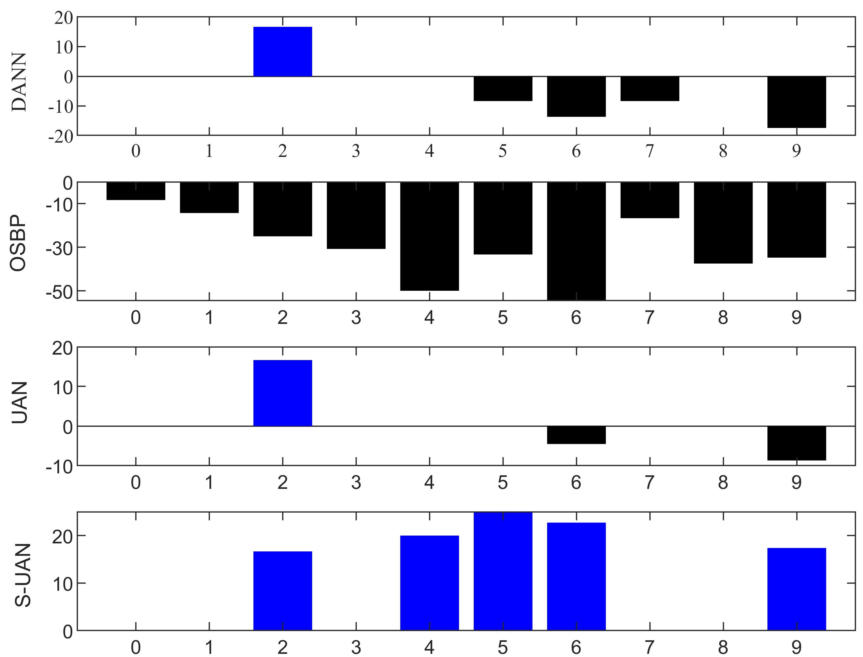
From Tables LABEL:Office-31 and LABEL:Office-Home, we can find that S-UAN outperforms all the compared methods. Particularly, we focus on the comparison with UAN [25]. Although UAN avoids negative transfer in most tasks, it still has negative transfer in some tasks. For example, Fig. 7 indicates the accuracy gain of each class compared to ResNet (no adaptation) on task $A\rightarrow D$. We can see that DANN, OSBP and UAN still suffer from negative transfer. Note that the accuracy of the label set $\{0,1,3,7,8\}$ arrives $100\%$ in ResNet. Except these classes, S-UAN avoids negative transfer and achieve widely positive transfer in all the classes. This is because S-UAN makes full use of the prediction information of the target data and employs class-wise weighting mechanism in the source domain.

Another perspective to analyze the classification results is the dimension-reduction of features. In general, low-dimensional distinguishable features are easier to distinguish in higher dimensions. To this end, we visualize features extracted from trained models by t-SNE tool. In Fig. 8, we compare S-UAN and UAN on task ImageNet-Caltech, which contains 84 common classes and 1173 total classes. Overall, the distinguishability of UAN features is not as good as S-UAN, so the classification accuracy of S-UAN is higher than UDA’s.

Effect of Varying Size of $\overline{\mathcal{C}}_{t}$. We explore the performance of methods mentioned in Section III-B with the different sizes of $\overline{\mathcal{C}}_{t}$ on $\operatorname{task}\mathbf{A}\rightarrow\mathbf{D}$ in Office31 dataset, note that $\overline{\mathcal{C}}_{s}$ also changes correspondingly with fixed $\left|\mathcal{C}_{s}\cup\mathcal{C}_{t}\right|$ and $\xi$. As shown in Fig. 9(a), S-UAN outperforms all the compared methods on all the sizes of $\overline{\mathcal{C}}_{t}$. Particularly, when $\left|\overline{\mathcal{C}}_{t}\right|=0,$ this UDA setting degenerates to the partial domain adaptation, where $\mathcal{C}_{t}\subset\mathcal{C}_{s}$, and when $\left|\overline{\mathcal{C}}_{t}\right|=21$, this UDA setting degenerates to the open set domain adaptation, where $\mathcal{C}_{s}\subset\mathcal{C}_{t},$ the performance of S-UAN is comparable to UAN’s. When $\left|\overline{\mathcal{C}}_{t}\right|$ vary between 0 and 21, which are the more general settings, S-UAN performs much better than UAN. When the size of $\overline{\mathcal{C}}_{t}$ appears in the middle of 0 and 21, S-UAN outperforms other methods with the largest margin. Generally, S-UAN produces better results with all size of $\overline{\mathcal{C}}_{t}$.

Effect of Varying Size of $\mathcal{C}$. We also explore the performance of these methods with different size of the common label set $\mathcal{C}$. The same task is used as before, and we have $|\mathcal{C}|+\left|\overline{\mathcal{C}}_{t}\right|+\left|\overline{\mathcal{C}}_{s}\right|=31.$ For simplicity, we let $\left|\overline{\mathcal{C}}_{t}\right|=\left|\overline{\mathcal{C}}_{s}\right|+1$ or $\left|\overline{\mathcal{C}}_{t}\right|=\left|\overline{\mathcal{C}}_{s}\right|$, and let $|\mathcal{C}|$ vary from 0 to 31. Fig. 9(b) shows the performance of these methods with different sizes of $|\mathcal{C}|$. When $|\mathcal{C}|=0$, there is no known class appearing in target domain, i.e. $\mathcal{C}_{t}\cap\mathcal{C}_{s}=\emptyset$. We see that the accuracy of S-UAN is similar to UDA’s. When $|\mathcal{C}|>0$, i.e. $\mathcal{C}_{t}\cap\mathcal{C}_{s}\neq\emptyset$, we find that S-UAN outperforms all the compared methods with large margins, revealing that class-wise weighting mechanism of proposed margin vector is more general and effective than sample-wise weighting mechanism in UDA.

In this section, we verify the properties of generalization bound by analyzing the target risk for task $\mathbf{A}\rightarrow\mathbf{D}$. We fix $|\mathcal{C}_{s}|=15$. ResNet, DANN, OSBP, UAN and S-UAN are compared in what follows.

Property 1: with fixed $|\mathcal{C}|$ and the increase of $|\mathcal{C}_{t}|$, the generalization bound increases when $|\mathcal{C}_{t}|<|\mathcal{C}_{s}|$. In this experiment, we fix $|\mathcal{C}|=10$ and set $|\mathcal{C}_{t}|$=10,13,15,20,25,26, correspondingly, $\gamma=1.50,1.15,1.00,0.75,0.60,0.58$. The experiment results are shown in Fig. 10(a), except DANN and OSBP, other well-behaved methods are all suffered from performance degradation with the increase of $|\mathcal{C}_{t}|$ when $\gamma>1$. And when $\gamma\leq 1$, the performance of three well-behaved methods does not vary obviously. This experimental result verifies the first property of Theorem 27. And we can find that the target risk of the proposed S-UAN is the lowest, which is the best learning algorithm for universal domain adaptation compared with the state-of-the-art domain adaptation methods.

Property 2: with the increase of $|\mathcal{C}|$, the generalization bound decreases. In this experiment, we fix $|\mathcal{C}_{t}|=15$ and set $|\mathcal{C}|=0,3,6,9,12,15$, correspondingly, $\alpha=0.0,0.2,0.4,0.6,0.8,1.0$, here $\gamma=1$. The experiment results are shown in Fig. 10(b), the sampling batch size $m=36$, we can see that the performance of all the methods is improved with the increase of $|\mathcal{C}|$ when $|\mathcal{C}|=\alpha|\mathcal{C}_{s}|\geq\frac{e}{2\max\{1,\gamma\}m}|\mathcal{C}_{s}|=0.57$. Note that $|\mathcal{C}|$ can only be an integer, although the generalization bound becomes higher when $|\mathcal{C}|$ varies from 0 to 0.57, we find that the value of generalization bound at $|\mathcal{C}|=1$ is lower than $|\mathcal{C}|=0$. This experimental result verifies the second property of Theorem 27. And the target risk of the proposed S-UAN is still the lowest of these methods.

Weight Analysis. To verify the inference introduced in Section I, we plot the estimated probability density distribution for different components of the $w^{s}(\mathbf{x})$ and $w^{t}(\mathbf{x})$ in Fig. 11. Results show that the distributions are well separated between shared and private label sets of both domains, explaining why S-UAN achieves stable performance in different UDA settings. We observe that distributions of source shared and private parts are much more distinguishable compared with UAN’s. And distributions of target shared and private parts are as distinguishable as UAN’s. Note that the definition of the weight of target samples is simple in S-UAN, but is also distinguishable enough for target shared and private parts.

Threshold Sensitivity. Although we have fixed the criterion for distinguishing unknown classes in all experiments, i.e. $w^{t}(\mathbf{x})\geq 0.5$. We also explore the sensitivity of the threshold for analysis. As shown in Fig. 12, though S-UAN’s accuracies vary by $2\sim 3\%$ with the change of the threshold, it achieves stable performance and outperforms other methods by large margins with the change of the threshold. Note that in our experiments, UAN’s accuracy on VisDA can’t reach their report in our experiments. However, S-UAN’s accuracies still outperform UAN’s reported accuracy, which is fully tuned and their best accuracy.

Hyperparameter Analysis. The only hyperparameter in S-UAN is the activated threshold $w_{0}$ of the normalized function as shown in Eq.10. The value of $w_{0}$ can be 0 or 1. When $w_{0}=0$, $w_{0}$ has no effect on Eq.10, and all the $w^{s}(\mathbf{x})$ $($or $w^{t}(\mathbf{x})$$)$ can be activated. When $w_{0}=1$, only the $w^{s}(\mathbf{x})$ $($or $w^{t}(\mathbf{x})$$)$ greater than the average value can be activated, and the remaining $w^{s}(\mathbf{x})$ $($or $w^{t}(\mathbf{x})$$)$ are set to 0. In the default settings of S-UAN, $w_{0}$ is set to 1 in Office-31 and VisDA, where $|\mathcal{C}_{s}|\geq|\mathcal{C}_{t}|$. And $w_{0}$ is set to 0 in Office-Home and ImageNet-Caltech, where $|\mathcal{C}_{s}|<|\mathcal{C}_{t}|$. To do ablation study on $w_{0}$, we also set $w_{0}=0$ in Office-31 and VisDA (S-UAN $\mathbf{w_{0}=0}$) in Table LABEL:Office-31. We can find that S-UAN outperforms all the compared methods, even if $w_{0}=0$ in all experiments.

References

- [1] K. Saenko, B. Kulis, M. Fritz, and T. Darrell, “Adapting visual category models to new domains,” in Proceedings of the European Conference on Computer Vision, ECCV, 2010, pp. 213–226.
- [2] L. Duan, I. W. Tsang, and D. Xu, “Domain transfer multiple kernel learning,” IEEE Trans. Pattern Anal. Mach. Intell., pp. 465–479, 2012.
- [3] K. Zhang, B. Schölkopf, K. Muandet, and Z. Wang, “Domain adaptation under target and conditional shift,” in Proceedings of the 30th International Conference on Machine Learning, ICML, 2013, pp. 819–827.
- [4] E. Tzeng, J. Hoffman, N. Zhang, K. Saenko, and T. Darrell, “Deep domain confusion: Maximizing for domain invariance,” CoRR, vol. abs/1412.3474, 2014.
- [5] M. Long, Y. Cao, J. Wang, and M. I. Jordan, “Learning transferable features with deep adaptation networks,” in Proceedings of the 32nd International Conference on Machine Learning, ICML, 2015, pp. 97–105.
- [6] Y. Ganin, E. Ustinova, H. Ajakan, P. Germain, H. Larochelle, F. Laviolette, M. Marchand, and V. S. Lempitsky, “Domain-adversarial training of neural networks,” J. Mach. Learn. Res., pp. 59:1–59:35, 2016.
- [7] P. Häusser, T. Frerix, A. Mordvintsev, and D. Cremers, “Associative domain adaptation,” in IEEE International Conference on Computer Vision, ICCV, 2017, pp. 2784–2792.
- [8] M. Long, H. Zhu, J. Wang, and M. I. Jordan, “Unsupervised domain adaptation with residual transfer networks,” in Advances in neural information processing systems, 2016, pp. 136–144.
- [9] E. Tzeng, J. Hoffman, K. Saenko, and T. Darrell, “Adversarial discriminative domain adaptation,” in IEEE Conference on Computer Vision and Pattern Recognition, CVPR, 2017, pp. 2962–2971.
- [10] K. Saito, K. Watanabe, Y. Ushiku, and T. Harada, “Maximum classifier discrepancy for unsupervised domain adaptation,” in IEEE Conference on Computer Vision and Pattern Recognition, CVPR, 2018, pp. 3723–3732.
- [11] M. Long, Z. Cao, J. Wang, and M. I. Jordan, “Conditional adversarial domain adaptation,” in Advances in Neural Information Processing Systems, 2018, pp. 1640–1650.
- [12] F. M. Carlucci, L. Porzi, B. Caputo, E. Ricci, and S. R. Bulò, “Autodial: Automatic domain alignment layers,” in IEEE International Conference on Computer Vision, ICCV, 2017, pp. 5077–5085.
- [13] S. Xie, Z. Zheng, L. Chen, and C. Chen, “Learning semantic representations for unsupervised domain adaptation,” in Proceedings of the 35th International Conference on Machine Learning, ICML, 2018, pp. 5419–5428.
- [14] Z. Murez, S. Kolouri, D. J. Kriegman, R. Ramamoorthi, and K. Kim, “Image to image translation for domain adaptation,” in 2018 IEEE Conference on Computer Vision and Pattern Recognition, CVPR, 2018, pp. 4500–4509.
- [15] R. Volpi, P. Morerio, S. Savarese, and V. Murino, “Adversarial feature augmentation for unsupervised domain adaptation,” in IEEE Conference on Computer Vision and Pattern Recognition, CVPR, 2018, pp. 5495–5504.
- [16] L. Hu, M. Kan, S. Shan, and X. Chen, “Duplex generative adversarial network for unsupervised domain adaptation,” in IEEE Conference on Computer Vision and Pattern Recognition, CVPR, 2018, pp. 1498–1507.
- [17] Q. Chen, Y. Liu, Z. Wang, I. J. Wassell, and K. Chetty, “Re-weighted adversarial adaptation network for unsupervised domain adaptation,” in IEEE Conference on Computer Vision and Pattern Recognition, CVPR, 2018, pp. 7976–7985.
- [18] Y. Ganin, E. Ustinova, H. Ajakan, P. Germain, H. Larochelle, F. Laviolette, M. Marchand, and V. Lempitsky, “Domain-adversarial training of neural networks,” The Journal of Machine Learning Research, vol. 17, no. 1, pp. 2096–2030, 2016.
- [19] Z. Cao, M. Long, J. Wang, and M. I. Jordan, “Partial transfer learning with selective adversarial networks,” in IEEE Conference on Computer Vision and Pattern Recognition, CVPR, 2018, pp. 2724–2732.
- [20] J. Zhang, Z. Ding, W. Li, and P. Ogunbona, “Importance weighted adversarial nets for partial domain adaptation,” in IEEE Conference on Computer Vision and Pattern Recognition, CVPR, 2018, pp. 8156–8164.
- [21] Z. Cao, L. Ma, M. Long, and J. Wang, “Partial adversarial domain adaptation,” in Proceedings of the European Conference on Computer Vision, ECCV, 2018, pp. 135–150.
- [22] C. Ren, P. Ge, P. Yang, and S. Yan, “Learning target-domain-specific classifier for partial domain adaptation,” IEEE Transactions on Neural Networks and Learning Systems, pp. 1–13, 2020.
- [23] K. Saito, S. Yamamoto, Y. Ushiku, and T. Harada, “Open set domain adaptation by backpropagation,” in Proceedings of the European Conference on Computer Vision, ECCV, 2018, pp. 153–168.
- [24] P. Panareda Busto and J. Gall, “Open set domain adaptation,” in Proceedings of the IEEE International Conference on Computer Vision, 2017, pp. 754–763.
- [25] K. You, M. Long, Z. Cao, J. Wang, and M. I. Jordan, “Universal domain adaptation,” in Proceedings of the IEEE Conference on Computer Vision and Pattern Recognition, 2019, pp. 2720–2729.
- [26] Y. Ganin and V. S. Lempitsky, “Unsupervised domain adaptation by backpropagation,” in Proceedings of the 32nd International Conference on Machine Learning, ICML, vol. 37, 2015, pp. 1180–1189.
- [27] V. Koltchinskii, D. Panchenko et al., “Empirical margin distributions and bounding the generalization error of combined classifiers,” The Annals of Statistics, vol. 30, no. 1, pp. 1–50, 2002.
- [28] Y. Zhang, T. Liu, M. Long, and M. I. Jordan, “Bridging theory and algorithm for domain adaptation,” arXiv preprint arXiv:1904.05801, 2019.
- [29] H. Liu, Z. Cao, M. Long, J. Wang, and Q. Yang, “Separate to adapt: Open set domain adaptation via progressive separation,” in Proceedings of the IEEE Conference on Computer Vision and Pattern Recognition, 2019, pp. 2927–2936.
- [30] D. Kifer, S. Ben-David, and J. Gehrke, “Detecting change in data streams,” in Proceedings of the Thirtieth International Conference on Very Large Data Bases, VLDB. Morgan Kaufmann, 2004, pp. 180–191.
- [31] J. Blitzer, K. Crammer, A. Kulesza, F. Pereira, and J. Wortman, “Learning bounds for domain adaptation,” in NeurIPS. Curran Associates, Inc., 2007, pp. 129–136.
- [32] W. Ochs, “On the strong law of large numbers in quantum probability theory,” J. Philos. Log., vol. 6, no. 1, pp. 473–480, 1977.
- [33] S. Ben-David, J. Blitzer, K. Crammer, A. Kulesza, F. Pereira, and J. W. Vaughan, “A theory of learning from different domains,” Mach. Learn., vol. 79, no. 1-2, pp. 151–175, 2010.
- [34] S. Ben-David, J. Blitzer, K. Crammer, and F. Pereira, “Analysis of representations for domain adaptation,” in NeurIPS. MIT Press, 2006, pp. 137–144.
- [35] K. Crammer, M. J. Kearns, and J. Wortman, “Learning from multiple sources,” J. Mach. Learn. Res., vol. 9, pp. 1757–1774, 2008.
- [36] K. Saenko, B. Kulis, M. Fritz, and T. Darrell, “Adapting visual category models to new domains,” in European conference on computer vision. Springer, 2010, pp. 213–226.
- [37] B. Gong, Y. Shi, F. Sha, and K. Grauman, “Geodesic flow kernel for unsupervised domain adaptation,” in 2012 IEEE Conference on Computer Vision and Pattern Recognition. IEEE, 2012, pp. 2066–2073.
- [38] H. Venkateswara, J. Eusebio, S. Chakraborty, and S. Panchanathan, “Deep hashing network for unsupervised domain adaptation,” in Proceedings of the IEEE Conference on Computer Vision and Pattern Recognition, 2017, pp. 5018–5027.
- [39] X. Peng, B. Usman, N. Kaushik, D. Wang, J. Hoffman, and K. Saenko, “Visda: A synthetic-to-real benchmark for visual domain adaptation,” in Proceedings of the IEEE Conference on Computer Vision and Pattern Recognition Workshops, 2018, pp. 2021–2026.
- [40] O. Russakovsky, J. Deng, H. Su, J. Krause, S. Satheesh, S. Ma, Z. Huang, A. Karpathy, A. Khosla, M. Bernstein et al., “Imagenet large scale visual recognition challenge,” International journal of computer vision, vol. 115, no. 3, pp. 211–252, 2015.
- [41] K. He, X. Zhang, S. Ren, and J. Sun, “Deep residual learning for image recognition,” in Proceedings of the IEEE conference on computer vision and pattern recognition, 2016, pp. 770–778.
- [42] J. Zhang, Z. Ding, W. Li, and P. Ogunbona, “Importance weighted adversarial nets for partial domain adaptation,” in Proceedings of the IEEE Conference on Computer Vision and Pattern Recognition, 2018, pp. 8156–8164.
- [43] L. Zhang, J. Fu, S. Wang, D. Zhang, Z. Dong, and C. L. Philip Chen, “Guide subspace learning for unsupervised domain adaptation,” IEEE Transactions on Neural Networks and Learning Systems, pp. 1–15, 2019.
- [44] Y. Liu, B. Du, W. Tu, M. Gong, Y. Guo, and D. Tao, “Logdet metric-based domain adaptation,” IEEE Transactions on Neural Networks and Learning Systems, pp. 1–15, 2020.
- [45] P. Wei, Y. Ke, and C. K. Goh, “Feature analysis of marginalized stacked denoising autoenconder for unsupervised domain adaptation,” IEEE Transactions on Neural Networks and Learning Systems, vol. 30, no. 5, pp. 1321–1334, 2019.
- [46] W. Deng, A. Lendasse, Y. Ong, I. W. Tsang, L. Chen, and Q. Zheng, “Domain adaption via feature selection on explicit feature map,” IEEE Transactions on Neural Networks and Learning Systems, vol. 30, no. 4, pp. 1180–1190, 2019.
- [47] R. Cai, J. Li, Z. Zhang, X. Yang, and Z. Hao, “Dach: Domain adaptation without domain information,” IEEE Transactions on Neural Networks and Learning Systems, pp. 1–13, 2020.
- [48] X. Shen, Q. Dai, S. Mao, F. Chung, and K. Choi, “Network together: Node classification via cross-network deep network embedding,” IEEE Transactions on Neural Networks and Learning Systems, pp. 1–14, 2020.
- [49] Z. Wang, B. Du, and Y. Guo, “Domain adaptation with neural embedding matching,” IEEE Transactions on Neural Networks and Learning Systems, vol. 31, no. 7, pp. 2387–2397, 2020.
- [50] J. Li, K. Lu, Z. Huang, L. Zhu, and H. T. Shen, “Heterogeneous domain adaptation through progressive alignment,” IEEE Transactions on Neural Networks and Learning Systems, vol. 30, no. 5, pp. 1381–1391, 2019.
- [51] I. J. Goodfellow, J. Pouget-Abadie, M. Mirza, B. Xu, D. Warde-Farley, S. Ozair, A. C. Courville, and Y. Bengio, “Generative adversarial nets,” in NeurIPS, 2014, pp. 2672–2680.
- [52] C. Wang, M. Niepert, and H. Li, “Recsys-dan: Discriminative adversarial networks for cross-domain recommender systems,” IEEE Transactions on Neural Networks and Learning Systems, pp. 1–10, 2019.
- [53] G. Cai, Y. Wang, L. He, and M. Zhou, “Unsupervised domain adaptation with adversarial residual transform networks,” IEEE Transactions on Neural Networks and Learning Systems, pp. 1–14, 2019.
- [54] A. Elisseeff and J. Weston, “A kernel method for multi-labelled classification,” in NeurIPS, 2001, pp. 681–687.
- [55] W. Liu and I. W. Tsang, “Large margin metric learning for multi-label prediction,” in Proceedings of the Twenty-Ninth AAAI Conference on Artificial Intelligence, 2015, pp. 2800–2806.
- [56] V. Koltchinskii and D. Panchenko, “Empirical margin distributions and bounding the generalization error of combined classifiers,” The Annals of Stats, vol. 30, no. 1, 2000.
- [57] M. Xu, Y. Li, and Z. Zhou, “Robust multi-label learning with pro loss,” IEEE Transactions on Knowledge and Data Engineering, pp. 1–1, 2019.
- [58] B. Jia and M. Zhang, “Maximum margin multi-dimensional classification,” in The Thirty-Fourth AAAI Conference on Artificial Intelligence, AAAI, 2020, pp. 4312–4319.
- [59] Y. Yin, Z. Yang, H. Hu, and X. Wu, “Metric-learning-assisted domain adaptation,” CoRR, vol. abs/2004.10963, 2020.