Unusual quasiparticles and tunneling conductance in quantum point contacts in fractional quantum Hall systems
Abstract
Understanding topological matter in the fractional quantum Hall (FQH) effect requires identifying the nature of edge state quasiparticles. FQH edge state at the filling factor in the spin-polarized and non-polarized phases is represented by the two modes of composite fermions (CF) with the parallel or opposite spins described by the chiral Luttinger liquids. Tunneling through a quantum point contact (QPC) in such systems between different or similar spin phases is solved exactly. With the increase of the applied voltage, the QPC conductance grows from zero and saturates at while a weak electron tunneling between the edge modes with the same spin transforms into a backscattering carried by the charge quasiparticles. These unusual quasiparticles and conductance plateau emerge in the QPC with one or two CF modes scattering into a single mode, as occurs in these systems. We propose experiments on the applied voltage and temperature dependence of the QPC conductance and noise that can shed light on the nature of edge states and FQH transport.
Quantum Hall effect (QHE) emerges in quantizing magnetic fields in a two-dimensional electron gas. It exhibits a zero longitudinal resistance and the Hall conductance quantized in terms of the number of conductance quanta , where is the electron charge and is the Planck constant. When electron correlations become important, the fractional quantum Hall effect (FQHE) exhibits a fractionally quantized conductance. FQHE excitations are fractionally charged quasiparticles that obey abelian or non-abelian anyon statistics Leinaas and Murheim (1977); Wilczek (1982a, b); Wilczek and Zee (1983); Halperin (1984); Arovas et al. (1984); Read and Green (2000). FQHE with its edge states is the remarkable breeding ground for the observation of topological phenomena and the creation of qubits for topological quantum computing Nayak et al. (2008); Lindner et al. (2012); Clarke et al. (2012); Vaezi (2013); Mong et al. (2014); Vaezi (2014); Simion et al. (2018); Liang et al. (2019); Hutzel et al. (2019); Tylan-Tyler and Lyanda-Geller (2015).
QHE conductance quantization in many cases stems from the edge state picture Halperin (1982) in the Landauer- Buttiker approach Büttiker (1988). For the FQHE, Wen Wen (1995) found that at filling factors of Laughlin Laughlin (1983) states , where is odd, is the electron density, is the external magnetic field, and is the flux quanta, the excitations on the edge of the 2D electron system can be described as the chiral Luttinger liquids. While in quantum wires Ponomarenko (1995); Maslov and Stone (1995); Safi and Schulz (1995) conductance does not depend on the Luttinger liquid parameters, the picture of chiral Luttinger liquids allowed to explain the quantized Hall conductance Wen (1995); Kane and Fisher (1992) and tunneling of edge states through the quantum point contact (QPC) Fendley et al. (1995a, b); Sandler et al. (1998). Furthermore, in Fendley et al. (1995a) the thermodynamic Bethe Anzatz and the integrability of the Luttinger model with impurity interaction were used to calculate the non-equilibrium temperature-dependent conductance and noise.
A more complex situation emerges for hierarchical FQHE states Haldane (1983); Girvin (1984); Halperin (1984), such as state, for which several models were proposed. Since this state is a hole-conjugate of the state, it was suggested in MacDonald (1990); Johnson and MacDonald (1991) that its edge state consists of an outer downstream integer mode (from the underlying state) and an inner, counterpropagating -1/3 edge mode. Consideration of a bilayer system in McDonald and Haldane (1996) discussed this conjugated state and two other models, two independent edge channels and a pseudospin singlet state. The importance of disorder scattering between edge modes was underscored in Kane et al. (1994); Kane and Fisher (1997), where it was shown that the scattering results in two decoupled modes, a single downstream charge mode with conductance and a counterpropagating neutral mode. Soft confining potential leads to a reconstructed edge involving the formation of strip and two downstream charge modes with conductance and counterpropagating neutral modes that were considered in Meir (1994); Wang et al. (2013). With different approaches to the structure of the edge, there have also been two approaches to transport. Conductance quantization implies equilibration between the chemical potentials of the reservoirs and the outgoing edges. The first approach, incoherent transport model, assumes a short coherent length and suppression of quantum interference between the channels Kane and Fisher (1995); Chamon and Fradkin (1997); Protopopov et al. (2017); Nosiglia et al. (2018); Spanslatt et al. (2020); the second approach is quantum solution taking interference into account Fendley et al. (1995a); Ponomarenko and Averin (2003). Experimentally, studies of tunneling through quantum point contacts (QPC) at in Bid et al. (2009); Baer et al. (2014); Sabo et al. (2017) have shown a conductance plateau at , however, recent work Nakamura et al. (2023) demonstrated its appearance within of .
In this paper, we find an exact quantum mechanical solution to the model of tunneling through QPC in several edge configurations. It exhibits the fractional charge of backscattering quasiparticles, and conductance plateau. One case when the model is realized is associated with the transition between spin-polarized and unpolarized FQH phases Eisenstein et al. (1990); Kraus et al. (2002); Wu et al. (2012) which occurs due to the crossing of the two composite fermion (CF) energy states Jain (1989, 2007) with opposite spin polarization Ronen et al. (2018); Kukushkin et al. (1999); Liang et al. (2019). It was recently shown Kazakov et al. (2016, 2017); Wu et al. (2018); Wang et al. (2021) that the two different spin phases can be induced in the neighboring regions of the FQH liquid by electrostatic gates. The properties of a contact between the regions naturally lead to the model with two CF edge modes of the spin-polarized phase coupled by electron tunneling through QPC at low voltage and temperature to one CF edge mode of the same spin in the unpolarized phase. The same model also describes tunneling through QPC between the FQH regions in the identical spin phases when two CF edge modes in one of those regions are well separated in space due to its potential profile so that only one mode can tunnel. The exact solution to the model shows that with an increase of the applied voltage or temperature, the QPC conductance grows from zero and saturates at while a weak electron tunneling between the edge modes with the same spin transforms into the backscattering carried by the charge quasiparticles. This confirms the conductance earlier found by us for the contact between spin-polarized and unpolarized regions using a strong coupling boundary conditions approach Wang et al. (2021). We show that the quasiparticle charge is also observable in the shot noise. Testing the predicted non-linear applied voltage dependence of the tunneling current, temperature dependence, and properties of the shot noise can distinguish coherent and incoherent transport models and uncover the physics of edges in both polarized and unpolarized FQHE at .
Model for edge states. The key point of our approach is the assumption of separation of the charge and neutral/spin edge modes due to the long-range Coulomb interaction, discussed in Wen (1995). We treat polarized and unpolarized phases of FQHE on equal footing describing edge states as chiral Luttinger liquids with action
| (1) |
where and are bosonic operators and and are velocities of the charge and the neutral modes, correspondingly. Their relation to electron edge modes corresponding to the two CF levels and to quasiparticle bosonic fields, properties of these operators, transformations between different representations, and underlying assumptions are discussed in the supplementary materials. The neutral operators describe the difference in the occupation numbers of -levels in the polarized phase and the spin density in the unpolarized phase. We will use the notation and for charge modes, and for neutral (spin) modes in the corresponding phases. We assume that no edge reconstruction takes place.
Tunneling and charge current. We begin with tunneling through a QPC between the polarized and unpolarized phases. In the weak coupling limit, it is carried by the whole electrons through the allowed spin-conserving processes involving the edge modes of the two CF levels in each phase. The point contact (junction) electron tunneling at between polarized and unpolarized phases is described by tunneling Hamiltonian
| (2) |
Here , ’s are Majorana fermions accounting for the fermion statistics of different CF edge modes and composing the corresponding Klein factors, and
| (3) |
where and are the CF fields, the tunneling amplitudes can be chosen real and positive, and is the applied voltage. We assume coherent propagation of charge and neutral (spin) modes along the edge and allow for the possibility of interference. The same tunneling Hamiltonian Eq. (2) can also describe tunneling between the two spin-polarized phases, with a single edge channel participating in tunneling, if the potential profile ensures that the second -level edge is located too far from the edge. Thus we study the QPC tunneling of two modes into one mode; tunneling of one mode into one mode will emerge for tunneling amplitude .
The tunneling charge current, from Eq. (2) is given by
| (4) |
where is the charge density, e=1. Its average and fluctuations are defined by the operators , whose evolution in the absence of tunneling is characterized by their second-order correlators. The latter are found from the Gaussian action Eq.(1) for , and similarly for and in the form
| (5) |
is the single point correlator at of a normalized chiral boson field, with action as in Eq.(1) for ,
| (6) |
Here , is the energy cut-off in both edges, and should be taken in the final results. In terms of the normalized chiral boson fields , the operators can also be represented as
| (7) |
which after fermionization
| (8) |
allows to re-write the tunneling Hamiltonian (2) as
| (9) |
leading to its interpretation as the tunneling process of electrons from the two non-interacting chiral channels into the FQHE edge of filling factor. Combining these interfering channels into a single tunneling channel and applying bosonization of its chiral fermion field
| (10) |
we obtain the tunneling Hamiltonian and current :
| (11) | |||
| (12) |
where , and the single Klein factor is omitted since its drops out from any perturbative order in due to the charge conservation.
The electron tunneling described by Eqs. (11,12) can be viewed as a single point electron tunneling between the two counterpropagating primary one-component edges of equal filling factor with densities and the corresponding electron annihilation operators . Here are normalized right and left moving chiral fields. Thus, the problem described by Eq.(2) maps onto and is equivalent to the problem of tunneling between the one-component edges and as described by Hamiltonian
| (13) |
The tunneling current in the latter problem coincides with in Eqs. (4,12). Its average was calculated in Fendley et al. (1995a). At finite temperatures this average is given by
| (14) |
where is the Fermi distribution function, and Weiss (1996). The integral in (14) is evaluated in terms of the imaginary part of the digamma-function Weiss et al. (1991):
| (15) |
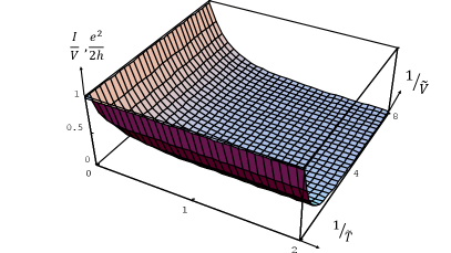
describing the dependence of tunneling current on the applied voltage and temperature in the whole range of parameters. In Fig.1 conductance is plotted as function of dimensionless variables and . At is given by
| (16) |
Tunneling current in various regimes. In order to elucidate different contributions to the tunneling current, we consider limiting cases of Eq. (16). In the regime of low , , of electron tunneling described by Eq. (13), the current is cubic in :
| (17) |
Therefore, we observe that in the coherent approach to transport, the behavior of tunneling current and conductance at small voltages is nonlinear in the applied voltage for , as opposed to the picture of incoherent transport Protopopov et al. (2017); Nosiglia et al. (2018); Spanslatt et al. (2020) that results in Landauer-Buettiker current linear in voltage and voltage-independent conductance.
In the regime of high voltages, , the exact Eq.(16) gives the following result for the average current, which we will denote :
| (18) |
The first term in this expression defines conductance . The second term corresponds to the reduction of the tunneling current defined by by the quasiparticle backscattering current
| (19) |
where .
In the supplement, we show an alternative way to calculate the tunneling currents using the strong coupling boundary conditions. We calculate the quasiparticle charge, and neutral and spin tunneling currents for tunneling through QPCs between polarized and unpolarized phases or between two polarized FQH liquids with one edge channel precluded from tunneling. The fermionization method above shows that tunneling of two interfering edge channels from one QPC side into a single channel on the other side is equivalent to a single tunneling channel with a renormalized tunneling amplitude.
We note that QPC conductance has been also discussed Nakamura et al. (2023) in terms of the incoherent equilibration model. However, neither the nonlinear current-voltage characteristics nor the temperature dependence following from Eq. (15) arise in that approach. has been also discussed for a special tunneling configuration, in which tunneling between two regions proceeds through the quantum dot with Lai and Yang (2013).
Quasiparticle charge. The reduction of tunneling current due to quasiparticle backscattering is described and their charge is determined by taking into account a sudden change of strong coupling boundary conditions at . For tunneling, e.g., between edge mode in the polarized region and edge mode with the same spin in the unpolarized region through the QPC at the strong coupling boundary conditions are given by
| (20) |
Here both fields are extended to finite from their expressions in Eq. (3), as chiral right moving fields. A sudden variation of the boundary conditions changes to ; both minimize . The boundary conditions also must keep continuous the two dual fields
| (21) | |||
| (22) |
where is the Heaviside step function. The jump from to leads to a jump in the dual fields
| (23) |
Since the corresponding jumps in these fields are given by
| (24) |
Then we get the change
| (25) |
Using the continuity condition
| (26) |
we find
| (27) |
Then the changes in the charge density and the density of the neutral mode are giiven by
| (28) |
In the supplement, we evaluate changes in tunneling densities of the spin mode in the unpolarized region and demonstrate relations between changes of densities for charge, neural and spin modes on both sides of the QPC.
As was shown in Ponomarenko and Averin (2004), the calculated transferred charge (28) enables us to identify the charge of backscattering quasiparticles. Here . Surprisingly, this charge is different from that one expects from Kane et al. (1994). This difference stems from the absence of tunneling between two edge states of opposite spin polarizations in the polarized and unpolarized regions, or, for tunneling between the regions with the same spin polarization, from a single channel participating in tunneling in at least one of the regions, due to a potential profile.
Shot noise. The experimental determination of the charge of the tunneling quasiparticles can be achieved by measurements of the shot nonequilibrium noise Saminadayar et al. (1997); De-Picciotto et al. (1997). The shot noise of the tunneling current Kane and Fisher (1994); Fendley et al. (1995a); Chamon et al. (1996); Lesage and Saleur (1997); Sandler et al. (1999) is given by
| (29) |
From Fendley et al. (1995a) it follows that
| (30) |
At small voltages and weak backscattering
| (31) |
At large voltages
| (32) |
The Schottky formula gives the charge of tunneling quasiparticles in the limits of weak electron tunneling and weak quasiparticle backscattering as the ratio of the corresponding values of noise to the currents, and . The resulting charge (writing e explicitly) is
| (33) |
Thus, the result for shot noise confirms the one obtained from the analysis of the sudden change in the boundary conditions: for tunneling at a filling factor through the QPC in our model, the quasiparticle charge is rather than the expected . We note that the noise signal arising in our model is much stronger than the noise in the incoherent equilibration model.
Discussion and conclusion. We have shown that the coherent quantum-mechanical model of transport in the FQHE, that potentially involves interference of chiral Luttinger liquid edge modes, leads to an exact solution of the problem of tunneling through the QPC between FQHE regions with different or similar spin phases. With the increase of the applied voltage, the QPC conductance grows from zero and saturates at while a weak electron tunneling through the QPC between the same spin edge modes transforms into the backscattering carried by the fractional charge quasiparticles. Unusual new quasiparticles and fractional conductance emerge in the QPC with one or two CF modes scattering into one mode as is the case in tunneling between polarized and unpolarized FQHE phases and can occur in tunneling between similar phases as a result of engineering the potential profile. Using the fermionization method, we have shown that tunneling of the two CF modes from one of the sides of the QPC is renormalized with the account of interference between the two modes, and is equivalent to tunneling of a single mode.
Recent experiments on QPC tunneling at have shown signatures of plateau. Besides our model this conductance can be discussed using the incoherent equilibration transport approach. However, then the non-linear current-voltage characteristics and temperature dependence of tunneling current and noise, which are predicted in the present work and can be tested experimentally, do not emerge in the incoherent model.
Acknowledgement. We are grateful to M. Manfra and L. Rokhinson for helpful discussions. YLG was supported by the U.S. Department of Energy, Office of Basic Energy Sciences, Division of Materials Sciences and Engineering under Award DE-SC0010544.
References
- Leinaas and Murheim (1977) J.M. Leinaas and J. Murheim, “On the theory of identical particles,” Nuovo Simento 37B, 1 (1977).
- Wilczek (1982a) F Wilczek, “Quantum mechanics of fractional-spin particles.” Phys. Rev. Lett. 40, 957–959 (1982a).
- Wilczek (1982b) Frank Wilczek, “Magnetic flux, angular momentum, and statistics,” Phys. Rev. Lett. 48, 1144–1146 (1982b).
- Wilczek and Zee (1983) F. Wilczek and A. Zee, “Linking numbers, spin, and statistics of solitons,” Phys. Rev. Lett. 51, 2250–2252 (1983).
- Halperin (1984) B.I. Halperin, “Statistics of quasiparticles and the hierarchy of fractional quantized Hall states,” Phys. Rev. Lett. 52, 1583–1586 (1984).
- Arovas et al. (1984) D.P. Arovas, J. R. Schrieffer, and F. Wilczek, “Fractional statistics and the quantum Hall effect,” Phys. Rev. Lett. 53, 722–723 (1984).
- Read and Green (2000) N. Read and D. Green, “Paired states of fermions in two dimensions with breaking of parity and time-reversal symmetries and the fractional quantum Hall effect,” Phys. Rev. B 61, 10267–10297 (2000).
- Nayak et al. (2008) C. Nayak, S. H. Simon, A. Stern, M. Freedman, and S. Das Sarma, “Non-abelian anyons and topological quantum computation,” Rev. Mod. Phys. 80, 1083 –1159 (2008).
- Lindner et al. (2012) N. Lindner, E. Berg, G. Refael, and A. Stern, “Fractionalizing Majorana fermions: Non-Abelian statistics on the edges of Abelian quantum Hall states,” Phys. Rev. X 2, 041002 (2012).
- Clarke et al. (2012) D. J. Clarke, J. Alicea, and K. Shtengel, “Exotic non-Abelian anyons from conventional fractional quantum Hall states,” Nat. Commun. 4, 1348 (2012).
- Vaezi (2013) Abolhassan Vaezi, “Fractional topological superconductor with fractionalized Majorana fermions,” Physical Review B 87, 035132 (2013).
- Mong et al. (2014) R. Mong, D. J. Clarke, J. Alicea, N. Lindner, P. Fendley, C. Nayak, Y. Oreg, A. Stern, E. Berg, and M. P. A. Shtengel, K.and Fisher, “Universal Topological Quantum Computation from a Superconductor-Abelian Quantum Hall Heterostructure,” Phys. Rev. X 4, 011036 (2014).
- Vaezi (2014) A. Vaezi, “Superconducting analogue of the parafermion fractional quantum Hall states,” Phys. Rev. X 4, 031009 (2014).
- Simion et al. (2018) G. Simion, A. Kazakov, L. P. Rokhinson, T. Wojtowicz, and Y. B. Lyanda-Geller, “Impurity-generated non-Abelions,” Phys. Rev. B 97, 245107 (2018).
- Liang et al. (2019) J. Liang, G. Simion, and Y. Lyanda-Geller, “Parafermions, induced edge states, and domain walls in fractional quantum Hall effect spin transitions,” Phys. Rev. B 100, 075155 (2019).
- Hutzel et al. (2019) W. Hutzel, J.J McCord, P.T. Raum, B Stern, H. Wang, V. W. Scarola, and M.R. Peterson, “A particle-hole-symmetric model for a paired fractional quantum Hall state in a half-filled Landau level,” Phys. Rev. B 99, 045126 (2019).
- Tylan-Tyler and Lyanda-Geller (2015) A. Tylan-Tyler and Y. Lyanda-Geller, “Phase diagram and edge states of the fractional quantum Hall state with Landau level mixing and finite well thickness,” Phys. Rev. B 91, 205404 (2015).
- Halperin (1982) B. I. Halperin, “Quantized Hall conductance, current-carring edge states, and the existance of extended states in a two-dimensional disordered potential,” Phys. Rev. B 25, 2185 (1982).
- Büttiker (1988) M. Büttiker, “Absence of backscattering in quantum Hall effect in multiprobe conductors,” Phys. Rev. B 38, 9375 (1988).
- Wen (1995) Xiao-Gang Wen, “Topological orders and edge excitations in fractional quantum Hall states,” Adv. Phys. 44, 405–473 (1995).
- Laughlin (1983) R. B. Laughlin, Phys. Rev. Lett. 50, 1395 (1983).
- Ponomarenko (1995) V.V. Ponomarenko, “Renormalization of the one-dimensional conductance in the Luttinger-liquid model,” Phys. Rev. B 52, R8666–8667 (1995).
- Maslov and Stone (1995) D. L. Maslov and M. Stone, “Landauer conductance of luttinger liquids with leads,” Phys. Rev. B 52, R5539–5542 (1995).
- Safi and Schulz (1995) I. Safi and H.J. Schulz, “Transport in an inhomogeneous interacting one-dimensional system,” Phys. Rev. B 52, R17040–17043 (1995).
- Kane and Fisher (1992) C.L Kane and M. P. A. Fisher, “Transmission through barriers and resonant tunneling in an interacting one-dimensional electron gas,” Phys. Rev. B 46, 15233–15262 (1992).
- Fendley et al. (1995a) P. Fendley, A. W. W. Ludwig, and H. Saleur, “Exact nonequilibrium dc shot noise in Luttinger liquids and fractional quantum hall devices,” Phys. Rev. Lett. 75, 2196–2199 (1995a).
- Fendley et al. (1995b) P. Fendley, A. W. W. Ludwig, and H. Saleur, “Exact nonequilibrium transport through point contacts in quantum wires and fractional quantum hall devices,” Phys. Rev. B 52, 8934–8950 (1995b).
- Sandler et al. (1998) N. P. Sandler, C. D. C. Chamon, and E. Fradkin, “Andreev reflection in the fractional quantum Hall effect,” Phys. Rev. B 57, 12324–12332 (1998).
- Haldane (1983) F. D. M. Haldane, “Fractional quantization of the Hall effect: A hierarchy of incompressible quantum fluid statesl,” Phys. Rev. Lett. 51, 605–608 (1983).
- Girvin (1984) S. M. Girvin, “Particle-hole symmetry in the anomalous quantum Hall effect.” Phys. Rev. B 29, 6012–6014 (1984).
- MacDonald (1990) A. H. MacDonald, “Edge states in the fractional quantum Hall effect regime,” Phys. Rev. Lett. 64, 220–223 (1990).
- Johnson and MacDonald (1991) M. D. Johnson and A. H. MacDonald, “Composite edges in the =2/3 fractional quantum Hall effect,” Phys. Rev. Lett. 67, 2060–2063 (1991).
- McDonald and Haldane (1996) I.A. McDonald and F.D.M Haldane, “Topological phase transition in the = 2/3 quantum Hall effect,” Phys. Rev. B 53, 15845 (1996).
- Kane et al. (1994) C. L. Kane, M. P. A. Fisher, and J. Polchinski, “Randomness at the edge: Theory of quantum Hall transport at filling ,” Phys. Rev. Lett. 72, 4129–4132 (1994).
- Kane and Fisher (1997) C. L. Kane and Matthew P. A. Fisher, Perspectives in Quantum Hall Effects (Wiley-Verlag GmbH, Berlin, 1997) pp. 109–159.
- Meir (1994) Y. Meir, “Composite edge states in the fractional quantum Hall regime,” Phys. Rev. Lett. 72, 2624 (1994).
- Wang et al. (2013) J. Wang, Y. Meir, and Y. Gefen, “Edge reconstruction in the fractional quantum Hall state,” Phys. Rev. Lett. 111, 246803 (2013).
- Kane and Fisher (1995) C.L Kane and M. P. A. Fisher, “Contacts and edge-state equilibration in the fractional quantum Hall effect,” Phys. Rev. B 52, 17393–17405 (1995).
- Chamon and Fradkin (1997) C. Chamon and E. Fradkin, “Distinct universal conductances in tunneling to quantum Hall states: The role of contacts,” Phys. Rev. B 56, 2012–2025 (1997).
- Protopopov et al. (2017) I. V. Protopopov, Y. Gefen, and A.D. Mirlin, “Transport in a disordered fractional quantum Hall junction.” Ann. Phys. 385, 287–327 (2017).
- Nosiglia et al. (2018) C. Nosiglia, J. Park, B. Rosenow, and Y. Gefen, “Incoherent transport on the quantum Hall edge,” Phys. Rev. B 78, 075308 (2018).
- Spanslatt et al. (2020) C. Spanslatt, J. Park, Y. Gefen, and A.D. Mirlin, “Conductance plateaus and shot noise in fractional quantum Hall point contacts,” Phys. Rev. B 101, 115408 (2020).
- Ponomarenko and Averin (2003) V. Ponomarenko and D. Averin, “Quantum coherent equilibration in multipoint electron tunneling into a fractional quantum Hall edge,” Phys. Rev. B 67, 035314 (2003).
- Bid et al. (2009) A. Bid, N. Ofek, M. Heiblum, V. Umansky, and D. Mahalu, “Shot noise and charge at the = 2/3 composite fractional quantum Hall state,” Phys. Rev. Lett. 103, 236802 (2009).
- Baer et al. (2014) S Baer, C Roessler, E.C. de Wiljes, P.L. Ardelt, T. Ihn, K. Ensslin, C. Reichl, and W. Wegscheider, “Interplay of fractional quantum Hall states and localization in quantum point contacts,” Phys. Rev. B 89, 085424 (2014).
- Sabo et al. (2017) R. Sabo, I. Gurman, A. Rosenblatt, F Lafont, D. Banitt, J. Park, M. Heiblum, Y. Gefen, V. Umansky, and D. Mahalu, “Edge reconstruction in fractional quantum Hall states,” Nature Physics 13, 491–496 (2017).
- Nakamura et al. (2023) J. Nakamura, S. Liang, Garndner G.S., and M.J. Manfra, “Half-integer condactance plateau at the fractional quantum Hall state in a quantum point contact,” Phys. Rev. Lett. 130, 076205 (2023).
- Eisenstein et al. (1990) J. Eisenstein, H. Stormer, L. Pfeiffer, and K. West, “Evidence for a spin transition in the fractional quantum Hall effect,” Phys. Rev. B 41, 7910–7913 (1990).
- Kraus et al. (2002) S. Kraus, O. Stern, J. G. S. Lok, W. Dietsche, K. von Klitzing, M. Bichler, D. Schuh, and W. Wegscheider, “From quantum Hall ferromagnetism to huge longitudinal resistance at the =2/3 fractional quantum Hall state,” Phys. Rev. Lett. 89, 266801 (2002).
- Wu et al. (2012) Ying-Hai Wu, G. J. Sreejith, and Jainendra K. Jain, “Microscopic study of edge excitations of spin-polarized and spin-unpolarized fractional quantum Hall effect,” Phys. Rev. B 86, 115127 (2012).
- Jain (1989) J. K. Jain, “Composite Fermion approach for the fractional quantum Hall effect,” Phys. Rev. Lett. 63, 199–202 (1989).
- Jain (2007) Jainendra K Jain, Composite fermions (Cambridge University Press, Cambridge, 2007).
- Ronen et al. (2018) Y. Ronen, Y. Cohen, D. Banitt, M. Heiblum, and V. Umansky, “Robust integer and fractional helical modes in the quantum Hall effect,” Nature Physics 14, 411–416 (2018).
- Kukushkin et al. (1999) I. V. Kukushkin, K. v. Klitzing, and K. Eberl, “Spin polarization of composite fermions: Measurements of the Fermi energy,” Phys. Rev. Lett. 82, 3665–3668 (1999).
- Kazakov et al. (2016) A. Kazakov, G. Simion, Y. Lyanda-Geller, V. Kolkovsky, Z. Adamus, G. Karczewski, T. Wojtowicz, and L. P. Rokhinson, “Electrostatic control of quantum Hall ferromagnetic transition: A step toward reconfigurable network of helical channels,” Phys. Rev. B 94, 075309 (2016).
- Kazakov et al. (2017) A. Kazakov, G. Simion, Y. Lyanda-Geller, V. Kolkovsky, Z. Adamus, G. Karczewski, T. Wojtowicz, and L. P. Rokhinson, “Mesoscopic transport in electrostatically defined spin-full channels in quantum Hall ferromagnets,” Phys. Rev. Lett. 119, 046803 (2017).
- Wu et al. (2018) T. Wu, Z. Wan, A. Kazakov, Y. Wang, G. Simion, J. Liang, K. W. West, K. Baldwin, L. N. Pfeiffer, Y. Lyanda-Geller, and L. P. Rokhinson, “Formation of helical domain walls in the fractional quantum Hall regime as a step toward realization of high-order non-Abelian excitations,” Phys. Rev. B 97, 245304 (2018).
- Wang et al. (2021) Y. Wang, V. Ponomarenko, Z. Wan, K.W. West, K.W. Baldwin, L.N Pfeiffer, Y. Lyanda-Geller, and L.P. Rokhinson, “Transport in helical Luttinger liquids in the fractional quantum Hall regime,” Nature Communications 12, 5312 (2021).
- Weiss (1996) U. Weiss, “Low-temperature conduction and dc current noise in a quantum wire with impurity,” Solid State Communications 100, 281–285 (1996).
- Weiss et al. (1991) U. Weiss, M Sasetti, T. Negele, and M. Wollensak, “Dissipative quantum dynamics in a multiwell system,” Z. Phys. B 84, 471–482 (1991).
- Lai and Yang (2013) H-H. Lai and K. Yang, “Distinguishing particle-hole conjugated fractional quantum Hall states using quantum-dot-mediated edge transport,” Phys. Rev. B 87, 125130 (2013).
- Ponomarenko and Averin (2004) V.V. Ponomarenko and D.V. Averin, “Strong-coupling branching between edges of fractional quantum Hall liquids,” Phys. Rev. B 70, 195316 (2004).
- Saminadayar et al. (1997) L. Saminadayar, D. Glattli, Y. Jin, and B. Etienne, “Observation of the e/3 fractionally charged Laughlin quasiparticle,” Phys. Rev. Lett. 79, 2526–2529 (1997).
- De-Picciotto et al. (1997) R. De-Picciotto, M. Reznikov, M. Heiblum, V. Umansky, and D. Bunin, G.and Mahalu, “Direct observation of fractional charge,” Nature 389, 162–164 (1997).
- Kane and Fisher (1994) C. L. Kane and M. P. A. Fisher, “Nonequilibrium noise and fractional charge in the quantum Hall effect,” Phys. Rev. B 72, 724–727 (1994).
- Chamon et al. (1996) C. D. C. Chamon, D. E. Freed, and X. G. Wen, “Nonequilibrium quantum noise in chiral Luttinger liquids,” Phys. Rev B 53, 4033–4053 (1996).
- Lesage and Saleur (1997) F. Lesage and H. Saleur, “Correlations in one-dimensional quantum impurity problems with an external field.” Nucl. Phys. B 490, 543–575 (1997).
- Sandler et al. (1999) N. P. Sandler, C.D.C Chamon, and E. Fradkin, “Noise measurements and fractional charge in fractional quantum Hall liquids,” Phys. Rev. B 59, 12521–12536 (1999).
Supplementary Materials
I Note on scope of the supplemental materials.
In the supplemental materials we discuss relations between different representations of edge tunneling modes, paricularly between electron edge modes corresponding to the two CF levels and quasiparticle bosonic fields, transformations between different representations, and underlying assumptions of our model. We also show an alternative way to calculate the tunneling currents using the strong coupling boundary conditions and calculate the quasiparticle charge, and neutral and spin tunneling currents for tunneling through QPCs between polarized and unpolarized phases or between two polarized FQH liquids with one edge channel precluded from tunneling. Finally, in addition to calculation of tunneling density of the charge mode in the main text, we evaluate changes in tunneling densities of the spin mode in the unpolarized region and demonstrate relations between changes of densities for charge, neural and spin modes on both sides of the QPC.
Notations used in the supplement.
All equations numbers of the supplementary materials are labeled by capital S. Citations numbers refer to the list of references in the main text.
II Modeling of tunneling through a quantum point contact at
II.1 Description of edges of state in terms of bosonic fields and quasiparticle bosonic fields
Luttinger liquid action for edge states in terms of bosonic fields of electron operators is written as
| (S1) |
and the charge density is
| (S2) |
where matrix and vector q are given by
| (S3) |
In the most general form the interaction matrix is defined by two different diagonal matrix elements and for intra-mode Coulomb interactions in the modes and the off-diagonal matrix element for inter-mode Coulomb interactions,
| (S4) |
The commutation relation is
| (S5) |
For composite fermion creation operators, we have
| (S6) |
and
| (S7) |
Luttinger liquid action in terms of quasiparticle bosonic fields , defined by is given by
| (S8) |
where
| (S9) |
The two sets of fields are orthogonal:
| (S10) |
The charge mode , and the neutral mode are expressed as follows:
| (S11) |
which in vector form reads , where the operation transposes a row vector into a column vector. The transformation matrix is given by
| (S12) |
and the following relations hold
| (S13) | |||||
| (S14) |
The neutral mode can be interpreted as a difference in the occupation of edge modes corresponding to the first and second -levels of composite fermions. The FQHE at can emerge in two spin polarization states, spin-polarized (p index) with two filled composite fermion -levels in the same spin state, and spin-uppolarized (u index) with two filled composite fermion -levels with two opposite spins. In the unpolarized phase it coincides with the spin density and we will use spin index instead of .
II.2 Description of edges of state in terms of separate charge and neutral/spin modes
In a seminal paper by Kane Fisher and Polchinsky [34], it was suggested that a significant role in the physics of is played by scatttering between oppositely propagating modes. However, both polarized and unpolarized phases must be treated on equal footing. This immediately raises a point that the edges in these phases are drastically different: there could be no elastic scattering leading to hybridization of two edge states emerging from the bulk composite fermion picture in the unpolarized phase, where these two edge sttes have opposite spin. We note that true spin system is much more restrictive in this regard compared to and pseudospin layered system, where tunneling is allowed between layers. To resolve this issue, we use observation by Wen Wen (1995) that at strong Coulomb interactions, a spin-charge (neutral-charge) separation occurs. Once we assume this separation takes place, the Luttinger liquid action in both spin-polarized and spin-unpolarized phases has the same form as Kane-Fisher-Polchinsky action.
Therefore we formulate Luttinger liquid action in terms of separate charge and neutral/spin modes. Using matrix defined Eq. (S12) the transformed matrix , given by Eq. (S3) becomes
| (S15) |
For the transformed matrix ,
| (S16) |
we obtain
| (S17) |
where in terms of couplings , and in Eq.(S4), matrix ements of coupling matrix are given by
| (S18) |
For equal diagonal intra-mode couplings the off-diagonal terms of the matrix vanish, , and the diagonal elements take the form , .As was discussed by Wen in Ref. [20], equal couplings of both composite fermion modes Eq.(S4) are the consequences of the long-range Coulomb interaction. [In the absence of the mechanism of electron scattering on impurities this equal coupling allows separation of charge and neutral modes in polarized phase and charge and spin modes for non-polarized phase.]
In order to distinguish Luttinger liquid modes in p and u phases, we characterize all modes, including bosonic electron modes, quasiparticle modes, and separated charge and neutral (spin) modes by indices p and u. The transformed action for the p phase is
| (S19) |
where and are velocities of charge and neutral modes in polarized phase, correspondingly. This action coincides with the one expressed in terms of the charge and neutral fields in [34], in the case if no electron scattering that leads to the composite fermion (CF) tunneling between the different modes and no coupling between modes takes place. The Luttinger liquid action in u phase is similar with spin modes entering instead of neural modes:
| (S20) |
where and are velocities of charge and spin modes, correspondingly. The spin mode determines the spin current in the u phase. In both phases, charge and neutral, or charge and spin modes separate.
The commutation relations for separated charge and neutral modes in the p phase are given by
| (S21) | |||||
| (S22) |
In the u phase, the commutation relatons for separated charge and spin modes are given by these equations with substitution , . To acquire non-zero average charge density and current, density of the charge mode is shifted, . A non-zero average appears due to a charge current injection,
| (S23) |
where V is the applied voltage. Then the average current carried by the edge is
| (S24) |
with as in Eq.(S3). The shift of the charge mode density is described by an addition to the Luttinger liquid action
| (S25) |
so that . The case of injection from the unpolarized phase into polarized phase, when is shifted due to applied voltage instead of , is described by Eqs. (S23-S25) with the change .
II.3 The Luttinger liquid action in the presence of both spin-polarized and spin-unpolarized phases.
The Luttinger liquid action for the edge states at consisting of the two phases, polarized p and unpolarized u, is given by
| (S28) | |||
| (S31) |
where 4x4 matrices
| (S32) |
with matrix defined by Supplementary Eq. (S3) and
| (S33) |
with matrix is defined by Supplementary Eq. (S4). For convenience, in order to keep the form of relations for the current as described above for both p and u phases, we reverse the sign of the quasiparticle field , so that , but .
III Tunneling current through the quantum point contact between polarized and unpolarized phases
The point contact tunneling between the polarized and unpolarized phases carried by composite fermions with the same spin polarization is described by the tunneling Hamiltonian and current :
| (S34) | |||
| (S35) |
In order to access the properties of the system, it is instructive to consider the tunneling current [26] in the strong coupling limit with account for weak backscattering [38].
III.1 Tunneling current in the strong coupling limit
Transformation of the two tunneling fields to the right-moving chiral fields is described as follows
| (S36) | |||
| (S37) |
The two non-tunneling fields orthogonal to fields (S37) are described by
| (S38) | |||
| (S39) |
The strong coupling boundary conditions of Eq. (11), intertwin and at crossing:
| (S40) |
and keep continuous the nontunneling fields and and the two dual fields
| (S41) | |||
| (S42) |
where is the Heaviside step function. In the presence of voltage V that produces the tunneling current and a density shift via the shift of in Eq.(S23), we have the following time-dependent averages:
| (S43) | |||
| (S44) |
Therefore
| (S45) | |||
| (S46) |
It then follows
| (S47) | |||
| (S48) |
and
| (S49) | |||
| (S50) |
Furthermore, the strong coupling boundary conditions yield the following averages in the presence of voltage for and :
| (S51) | |||
| (S52) |
It then follows for the time-dependent averages and currents in the polarized region:
| (S53) | |||
| (S54) |
and
| (S55) | |||
| (S56) |
We observe that tunneling charge current from polarized region coincides with tunneling spin current current:
| (S57) |
and is opposite in sign to reflected neutral current in polarized region.
III.2 Reduction of tunneling current due to backscattering
Quasiparticle tunneling results in backscattering that reduces the tunneling current. Backscattering is associated with a sudden change at of the strong coupling boundary conditions
| (S58) |
from integer to integer that both minimize . This leads to a jump in the fields
| (S59) |
Since
| (S60) |
the corresponding jumps in the fields are given by
| (S61) |
that lead to the following changes
| (S62) |
At the same time,
| (S63) |
Then
| (S64) |
and the change of the charge density . Analogously, the change in spin mode
| (S65) |
and the change of the spin density
| (S66) |
Furthermore, from we get the change
| (S67) |
Using the continuity condition
| (S68) |
we find
| (S69) |
and for the change in the charge density and in the density of the neutral mode
| (S70) | |||
| (S71) |
As was shown in [62], the calculated transferred charge enables us to identify the charge of backscattering quasiparticles q=e/2. Surprisingly, this charge is different from q=e/3 which one expects from [34] . This difference stems from the absence of tunneling between two edge states of different spin polarizations in the polarized and unpolarized regions.
These calculations demonstrate that for tunneling through the QPC, in which one CF edge on one side of the QPC is scattered into one CF edge on the other side of the QPC the quasiparticle charge is and the conductance saturates at . This occurs in tunneling between both spin-like states of the polarized and unpolarized region or when the confining potential is engineered to allow only one mode to tunnel between two polarized or two unpolarized regions.