\floatsetup

[table]capposition=top

Unsupervised Restoration of Weather-affected Images using Deep Gaussian Process-based CycleGAN

Rajeev Yasarla Vishwanath A. Sindagi Vishal M. Patel
Johns Hopkins University
Department of Electrical and Computer Engineering, Baltimore, MD 21218, USA
{ryasarl1, vishwanathsindagi, vpatel36}@jhu.edu equal contribution

Abstract

Existing approaches for restoring weather-degraded images follow a fully-supervised paradigm and they require paired data for training. However, collecting paired data for weather degradations is extremely challenging, and existing methods end up training on synthetic data. To overcome this issue, we describe an approach for supervising deep networks that is based on CycleGAN, thereby enabling the use of unlabeled real-world data for training. Specifically, we introduce new losses for training CycleGAN that lead to more effective training, resulting in high quality reconstructions. These new losses are obtained by jointly modeling the latent space embeddings of predicted clean images and original clean images through Deep Gaussian Processes. This enables the CycleGAN architecture to transfer the knowledge from one domain (weather-degraded) to another (clean) more effectively. We demonstrate that the proposed method can be effectively applied to different restoration tasks like de-raining, de-hazing and de-snowing and it outperforms other unsupervised techniques (that leverage weather-based characteristics) by a considerable margin.

I Introduction

Weather conditions such as rain, fog (haze) and snow are aberrations in the environment that adversely affect the light rays traveling from the object to a visual sensor [1, 2, 3, 4, 5, 6]. This typically causes detrimental effects on the images captured by the sensors, resulting in poor aesthetic quality. Additionally, such images also reduce the performance of down-stream computer vision tasks such as detection and recognition [7]. Such tasks are often critical parts in autonomous navigation systems, which emphasizes the need to address these degradations. These reasons has motivated a plethora of research on methods to remove such effects.

Refer to caption — Figure 1: Results ( $\tilde{I}_{c}$ ) of the forward mapping ( $\mathcal{F}_{W\rightarrow C}$ ) network on a sample rain image for the deraining task from Cyc-GAN (top-row) and DGP-Cyc-GAN (bottom-row) at different epochs. These images are used as input to the reverse mapping network $\mathcal{F}_{C\rightarrow W}$ . Note that these images are noisy in the initial epochs which leads to incorrect training. Using Deep-GP, we are able to estimate the uncertainty which is in-turn incorporated into the loss function through a multiplier, resulting in the use of only non-noisy samples for the supervision. Hence, the proposed method outputs progressively cleaner outputs with lower uncertainty.

Recent research on weather-based restoration (de-raining, de-hazing and de-snowing) is typically focused on designing convolutional neural network (CNN)-based pixel-to-pixel regression architectures. These works typically incorporate different aspects such as attention [8, 9], degradation characteristics [10, 11], and many more. While these approaches have been effective in achieving high-quality restorations, they essentially follow a fully-supervised paradigm. Hence, they require paired data to successfully train their networks. Considering that weather effects are naturally occurring phenomena, it is practically infeasible to collect data containing pairs of clean and weather-affected (rainy, hazy, snowy) images. Due to this issue, existing restoration networks are unable to leverage real-world data, and they end up training on synthetically generated paired data. However, networks trained on synthetic datasets suffer distributional shift due to which they perform poorly on real-world images.

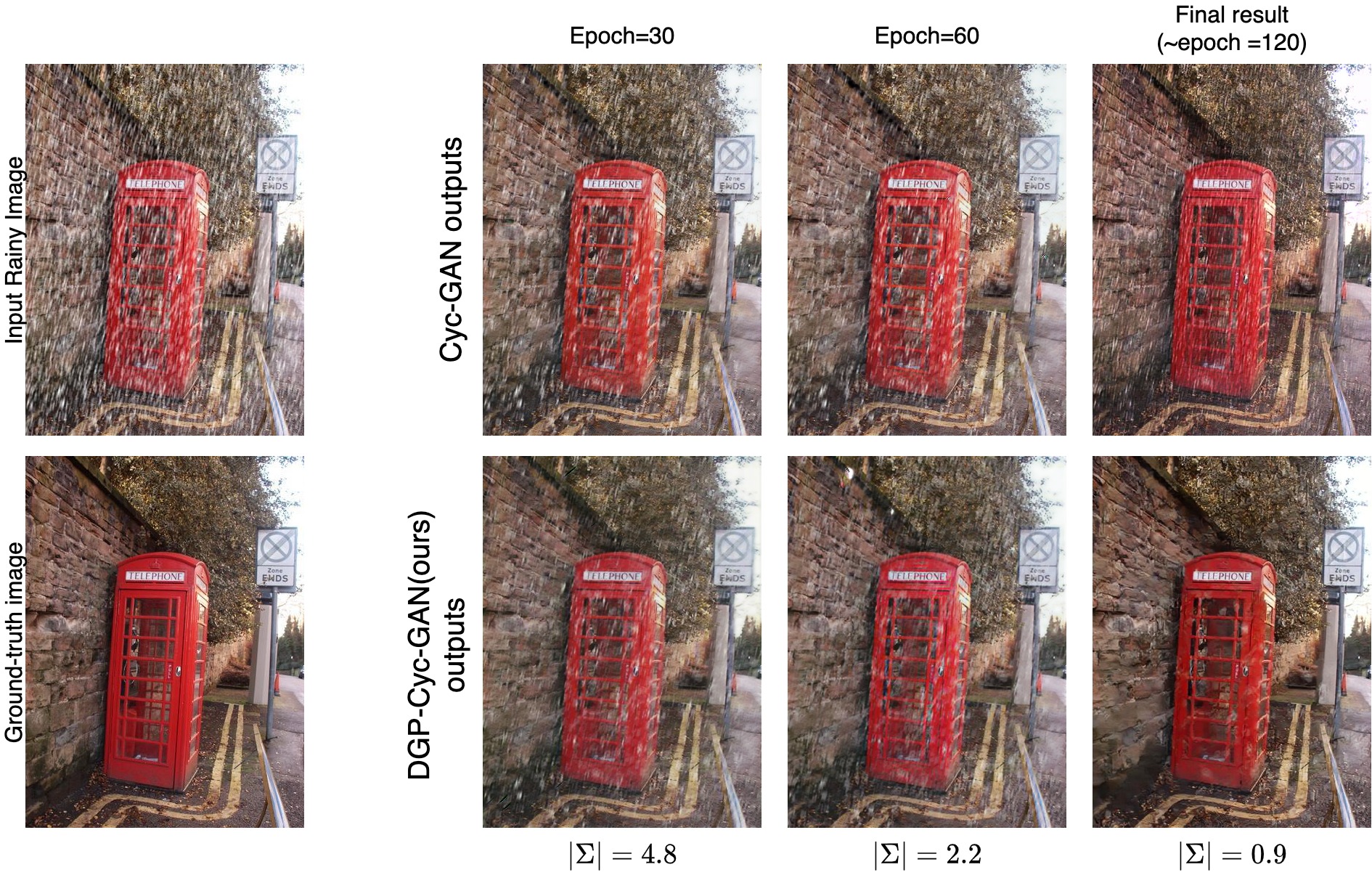
In this work, we address this issue by describing an approach to train a network from a set of degraded and clean images which are not paired. We view the restoration problem as a task of translation from one domain (weather-affected) to another (clean) and build on a recent popular method - CycleGAN [12]. One may train a network with unpaired data by ensuring that the restored images belong to the same distribution as that of real clean images [13]. However, the problem of translating images from one domain to another using unpaired data is ill-posed, as many mappings may satisfy this constraint. CycleGAN addresses this issue by using a forward mapping (clean to weather-affected) and a reverse mapping network (weather-affected to clean), and introduces an additional constraints via cycle-consistency losses along with adversarial losses . It is important to note that for computing the consistency losses, the output of the forward mapping function is used as input to the reverse mapping function and vice versa. However, during the initial stages of the training process, these outputs are potentially noisy which can be detrimental to learning an accurate function to map a degraded image to clean image (see Fig. 1 for details).

To overcome this issue, we introduce a new set of losses that provide additional supervision for predicted clean images in the latent space. These losses are derived by jointly modeling the latent projections of clean images and predicted clean images using Deep Gaussian Processes (GP). By conditioning this joint distribution on the projections of clean images, we are able to obtain pseudo-labels for the predicted clean images in the latent space. These pseudo-labels are then used in conjunction with the uncertainty derived from Deep-GP, to supervise the restoration network in the latent space. The use of uncertainty information ensures that only confident pseudo-labels are used during the training process. In other words, the noisy labels are disregarded, thus avoiding their use in the training of the forward and the reverse mapping networks in CycleGAN. To demonstrate the effectiveness of the proposed method, we conducted extensive experiments on multiple weather related restoration tasks like de-raining, dehazing and de-snowing using several benchmark datasets.

Following are the main contributions of our work:

•

We address the problem of learning to restore images for different weather conditions from unpaired data. Specifically, we present Deep Gaussian Processes-based CycleGAN that introduces new losses for training the CycleGAN architecture resulting in high quality restorations.
•

The proposed method achieves significant improvements over CycleGAN and other unsupervised techniques for various restoration tasks like as de-raining, de-hazing and de-snowing.
•

We show that the proposed method is able to leverage real-world data better as compared to CycleGAN by performing evaluation on a down-stream task, namely object detection on the restored images.

II Related Work

Image restoration for weather-degradations: Restoring weather-degraded images is a challenging problem since it is an ill-posed task even when paired data is available. Typically, these degradations are modeled based on the principles of physics, and the solutions are obtained using these physics-based models. Due to differences in the weather characteristics and the models, most existing approaches address these conditions separately. For example:

1.

Rain: A rainy image follows an additive model, where it is expressed as a superposition of a clean image and rain streaks [1, 2, 8, 14, 15, 16, 17, 18, 19, 20, 21]. Existing approaches for de-raining incorporate various aspects into their network design such as rain characteristics [14], attention [8, 22], context-awareness [23], depth information [24], and semi-supervised learning[25, 26]. A comprehensive analysis of these methods can be found in [27, 28].
2.

Haze: A hazy image is modeled as a superposition of a transmission map and an attenuated clean image [3, 4, 11, 7]. Like de-raining techniques, approaches developed for image de-hazing exploit different concepts such as multi-scale fusion [29, 30, 31, 32], gated fusion [33], network design [34], prior-information [10, 11, 35], adversarial loss [36, 37], image-to-image translation [38], and attention-awareness [9]. For more details, the readers are referred to [39, 40].
3.

Snow: A Snowy image is modeled similar to that of a rainy image, however the characteristics of snow-residue are quite distinct from rain-residue [5, 6]. Hence, approaches like [41, 42, 43] exploit various properties of snow to perform high-quality de-snowing.

While these approaches are able to achieve superior restoration quality, they essentially follow a fully-supervised paradigm and cannot be used for training on unpaired data. Additionally, these techniques are weather-specific as they incorporate weather-related models pertaining to a particular weather condition. In contrast, we propose a more general network that can be trained on unpaired data for any weather condition.

Unpaired image-to-image translation: Initial approaches for image-to-image translation [44, 45] are based on generative adversarial networks [13]. However, these methods employ paired data to train their networks. To overcome this issue, several techniques [12, 46, 47, 48] have been proposed for training networks with unpaired data. Zhu et al.[12] proposed CycleGAN which introduced cycle-consistency loss to impose an additional constraint that each image should be reconstructed correctly when translated twice. The objective is to conserve the overall structure and content of the image. DualGAN [46] and DiscoGAN [48] follow a similar approach, with slightly different losses. In contrast, approaches like [49, 47] consider a shared-latent space and they learn a joint distribution over images from two domains. They assume that images from two domains can be mapped into a low-dimensional shared-latent space. Most of the subsequent works [50, 51, 52, 53, 54] build on these approaches by incorporating additional information or structure like domain/feature disentanglement [50, 51], attention-awareness [52], learning of domain invariant representation [53] and instance-awareness [54].

Unpaired restoration for weather-degradations: Compared to fully-supervised approaches, research on unpaired restoration (for weather-degradations) has received limited attention. Most of the existing efforts are inspired by the unpaired translation approaches like CycleGAN [12] and DualGAN [46]. These approaches typically exploit weather-specific characteristics, and hence are designed individually for different weather conditions. For example, de-raining approaches like [55, 56, 57, 58] use rain properties to decompose the de-raining problem into foreground/background separation and employ rain-mask to provide additional supervision to train the CycleGAN network. Similarly, de-hazing approaches like [59, 60, 37] extend CycleGAN by incorporating haze related features. For example, Yang et al.[37] and Dudhane et al.[60] employ physics-based haze model to improve disentanglement and reconstruction in CycleGAN. Since these are designed specifically for a particular weather condition, they do not generalize to other conditions. In contrast, we propose a more general method that does not assume any specific weather-related model or characteristics. We enforce additional supervision during the training of CycleGAN which enables us to learn more accurate restoration functions resulting in better performance.

III Proposed method

Preliminaries: We are given a dataset of unpaired data, $\mathcal{D}=\mathcal{D}_{w}\cup\mathcal{D}_{c}$ , where $\mathcal{D}_{w}=\{I_{w}^{i}\}_{i=1}^{N}$ consists of a set of images degraded due to a particular weather condition and $\mathcal{D}_{c}=\{I_{c}^{i}\}_{i=1}^{N}$ consists of a set of clean images. The goal is to learn a restoration function $\mathcal{F}_{W\rightarrow C}$ , that maps a weather-degraded image ( $I_{w}$ ) to a clean image ( $I_{c}$ ). Since CycleGAN [12] enables training from unpaired data, we use this approach as a starting point to learn this function. In the CycleGAN framework, restoration function $\mathcal{F}_{W\rightarrow C}$ corresponds to the forward mapping network. As discussed earlier, CycleGAN enforces two constraints: (i) the distribution of restored images $P(\tilde{I_{c}})$ is similar to that of clean images $P(I_{c})$ and this is achieved with the aid of adversarial loss [13], (ii) In addition to $\mathcal{F}_{W\rightarrow C}$ , it also learns a reverse mapping function $\mathcal{F}_{C\rightarrow W}$ and ensures cycle consistency which is defined as: $\mathcal{F}_{C\rightarrow W}(\mathcal{F}_{W\rightarrow C}(I_{w}))=I_{w}$ .

In order to achieve high restoration quality, we need to learn an accurate restoration function ( $\mathcal{F}_{W\rightarrow C}$ ). Although CycleGAN enforces the aforementioned constraints, these are not necessarily sufficient. This is because, in the case of CycleGAN, the results ( $\tilde{I}_{c}$ ) of the forward mapping ( $\mathcal{F}_{W\rightarrow C}$ ) network are used as input to the reverse mapping network $\mathcal{F}_{C\rightarrow W}$ . These images are typically noisy in the initial epochs, as shown in Fig. 1 which leads to incorrect supervision and the network will overfit to the noisy data. In this work, we attempt to provide additional supervision via a set of new losses to overcome the aforementioned issues, thereby resulting in better restoration quality.

Further, although our method is based on CycleGAN, we demonstrate that it can be applied to other unpaired translation approaches like UNIT GAN (see supplementary). In what follows, we describe the proposed approach in detail.

Deep Gaussian Process-based CycleGAN: Fig. 2 shows an overview of the proposed method. As it can be observed, we build on CycleGAN. We introduce additional losses in the latent space for the forward and reverse mapping (as shown in red color). We extract latent space embeddings from two intermediate layers ( $\mathbf{s}$ and $\mathbf{z}$ ) in both the networks (forward mapping and reverse mapping). That is, in the forward mapping network ( $\mathcal{F}_{W\rightarrow C}$ ), a weather-degraded image $I_{w}$ is mapped to a latent embedding $\mathbf{s_{w}}$ , which is then mapped to another embedding $\mathbf{z_{w}}$ , before being mapped to restored (clean) image $\tilde{I}_{c}$ . The restored (cleaned) image $\tilde{I}_{c}$ is then forwarded through the reverse mapping network ( $\mathcal{F}_{C\rightarrow W}$ ) to produce latent vectors $\mathbf{\tilde{s}_{c}}$ and $\mathbf{\tilde{z}_{c}}$ , before being mapped to a reconstructed weather-degraded image $\hat{I}_{w}$ . Similarly, a clean image $I_{c}$ is mapped to a latent embedding $\mathbf{s_{c}}$ , which is then mapped to another embedding $\mathbf{z_{c}}$ , before being mapped to reconstructed weather-degraded image $\tilde{I}_{w}$ .

For learning to reconstruct $\tilde{I}_{c}$ , CycleGAN provides supervision by enforcing cycle consistency ( $L_{fwd}^{cyc}=|I_{w}-\hat{I}_{w}|_{1}$ ) and adversarial loss ( $L_{fwd}^{adv}(I_{c},\tilde{I}_{c})$ ). In order to ensure appropriate training, we provide additional supervision in the latent space by deriving pseudo-labels for the latent projection $\mathbf{\tilde{z}}_{c}$ of $\tilde{I}_{c}$ . The pseudo-label $\mathbf{\tilde{z}}^{p}_{c}$ is obtained by expressing the latent vectors of restored clean images $\tilde{I}_{c}$ in terms of projections of the original clean images $I_{c}$ by modeling joint distribution using Gaussian Process (GP). That is, given a set of “clean image” latent vectors $\mathbf{s}_{c}$ , from the first intermediate layer in the deep network, we write $\textbf{z}_{c}$ (latent vector of “clean images” from second intermediate layer) as a function of $\mathbf{s}_{c}$ as $\mathbf{z}_{c}=\mathbf{f}_{cw}\left(\mathbf{s}_{c}\right)$ . Hence, for the “restored clean image” latent vectors $\mathbf{\tilde{s}}_{c}$ , we can obtain the corresponding $\mathbf{\tilde{z}}_{c}^{p}$ using: $\mathbf{\tilde{z}}^{p}_{c}=\mathbf{\tilde{f}}_{cw}\left(\mathbf{\tilde{s}}_{c}\right).$

We aim to learn the function $\mathbf{\tilde{f}}_{cw}$ via Gaussian Processes. Specifically, we formulate the joint distribution of $\mathbf{{f}}_{cw}$ and $\mathbf{\tilde{f}}_{cw}$ (or correspondingly $\mathbf{{z}}_{c}$ and $\mathbf{\tilde{z}}^{p}_{c}$ ) as follows:

$\left[\begin{array}[]{l}\mathbf{f}_{cw}\\ \mathbf{\tilde{f}}_{cw}\end{array}\right]=\left[\begin{array}[]{l}\mathbf{z}_{c}\\ \mathbf{\tilde{z}}^{p}_{c}\end{array}\right]=\mathcal{N}\left(\left[\begin{array}[]{l}\boldsymbol{\mu}_{c}\\ \boldsymbol{\tilde{\mu}}_{{c}}\end{array}\right],\left[\begin{array}[]{cc}K\left(\mathbf{s}_{c},\mathbf{s}_{c}\right)&K\left(\mathbf{s}_{c},\mathbf{\tilde{s}}_{c}\right)\\ K\left(\mathbf{\tilde{s}}_{c},\mathbf{s}_{c}\right)&K\left(\mathbf{\tilde{s}}_{c},\mathbf{\tilde{s}}_{c}\right)\end{array}\right]+\sigma_{\epsilon}^{2}\mathbb{I}\right).$

(1)

Here, $K$ is the kernel matrix $K(\mathbf{U},\mathbf{V})_{i,j}=k(\mathbf{u}_{i},\mathbf{v}_{j})$ , where $\mathbf{u}_{i}$ is the $i^{th}$ vector of $\mathbf{U}$ and $\mathbf{v}_{j}$ is the $j^{th}$ vector of $\mathbf{V}$ , and $\mathbb{I}$ is identity matrix, $\sigma_{\epsilon}^{2}$ is the additive noise variance that is set to 0.01. By conditioning the above distribution, we obtain the following distribution for $\mathbf{z}^{p}_{c}$ :

P\left(\mathbf{\tilde{z}}^{p}_{c}|\mathbf{X}^{z}_{c},\mathbf{X}^{s}_{c},\mathbf{\tilde{s}}_{c}\right)=\mathcal{N}\left(\boldsymbol{\tilde{\mu}}_{c},\mathbf{\tilde{\Sigma}}_{{c}}\right),

(2)

where, $\mathbf{X}^{s}_{c}$ and $\mathbf{X}^{z}_{c}$ are matrices of latent projections $\mathbf{s}_{c}$ ’s and $\mathbf{z}_{c}$ ’s, respectively of all clean images in the dataset, and $\boldsymbol{\tilde{\mu}}_{c},\mathbf{\tilde{\Sigma}}_{{c}}$ are defined as follows:

$\begin{aligned} \boldsymbol{\tilde{\mu}}_{{{c}}}&=K\left(\mathbf{\tilde{s}}_{c},\mathbf{X}^{s}_{c}\right)\left[K\left(\mathbf{X}^{s}_{c},\mathbf{X}^{s}_{c}\right)+\sigma_{\epsilon}^{2}\mathbb{I}\right]^{-1}\mathbf{X}^{z}_{c},\\ \mathbf{\tilde{\Sigma}}_{{{c}}}&=K\left(\mathbf{\tilde{s}}_{c},\mathbf{\tilde{s}}_{c}\right)-K\left(\mathbf{\tilde{s}}_{c},\mathbf{X}^{s}_{c}\right)\left[K\left(\mathbf{X}^{s}_{c},\mathbf{X}^{s}_{c}\right)+\sigma_{\epsilon}^{2}\mathbb{I}\right]K\left(\mathbf{X}_{s_{c}},\mathbf{\tilde{s}}_{c}\right)+\sigma_{\epsilon}^{2}\mathbb{I}.\\ \end{aligned}$

(3)

We use the squared exponential kernel:

k\left(\mathbf{x}_{i},\mathbf{x}_{j}\right)=\beta^{2}\exp\left(-\frac{\left\|x_{i}-x_{j}\right\|^{2}}{2\gamma^{2}}\right),

(4)

where $\beta$ is the signal magnitude and $\gamma$ is the length scale. In all our experiments, we use $\frac{\beta}{\gamma}=1.0$ .

Considering that Deep Gaussian Processes have better representation power [61] as compared to single layer Gaussian Processes, we model $\left[\begin{array}[]{c}\mathbf{f}_{cw}\\ \tilde{\mathbf{f}}_{cw}\end{array}\right]$ using Deep GP with $L$ layers as follows:

$\displaystyle\mathbf{\bar{f}}_{cw}=\left[\begin{array}[]{c}\mathbf{f}_{cw}\\ \tilde{\mathbf{f}}_{cw}\end{array}\right]$	$\displaystyle\sim GP\left(\boldsymbol{\mu}^{L}_{f},K^{L}\left(\mathbf{h}^{L-1},\mathbf{h}^{L-1}\right)\right),$	(5)
$\displaystyle\mathbf{h}^{l}$	$\displaystyle\sim GP\left(\boldsymbol{\mu}^{l}_{h},K^{l}\left(\mathbf{h}^{l-1},\mathbf{h}^{l-1}\right)\right),$
$\displaystyle\mathbf{h}^{1}$	$\displaystyle\sim GP\left(\mathbf{\mu}^{1}_{h},K^{1}\left(\mathbf{s}_{c},\mathbf{s}_{c}\right)\right),$

where, $l$ indicates the layer index and $\mathbf{h}^{l}$ indicates the $l^{th}$ hidden layer. The use of Deep GPs along with convolutional neural networks (CNNs) is inspired by the works of [62, 63, 64]. The joint distribution can be written as:

$\begin{aligned} P\left(\mathbf{\bar{f}},\mathbf{h}^{1:L}|\mathbf{X}^{z}_{c},\mathbf{X}^{s}_{c},\mathbf{\tilde{s}}_{c}\right)=P\left(\mathbf{f}|\mathbf{h}^{L}\right)&P\left(\mathbf{h}^{L}|\mathbf{h}^{L-1}\right)\ldots\\ &\ldots P\left(\mathbf{h}^{1}|\mathbf{X}^{z}_{c},\mathbf{X}^{s}_{c},\mathbf{\tilde{s}}_{c}\right)\end{aligned}.$

(6)

Marginalizing the above distribution over $\mathbf{h}$ , we obtain:

P(\mathbf{f}|\mathbf{X}^{z}_{c},\mathbf{X}^{s}_{c},\mathbf{\tilde{s}}_{c})=\int P\left(\mathbf{f},\mathbf{h}^{1:L}|\mathbf{X}^{z}_{c},\mathbf{X}^{s}_{c},\mathbf{\tilde{s}}_{c}\right)d\mathbf{h}^{1:L}.

(7)

We approximate Deep GP with a single layer GP as described in [65]. More specifically, the authors in [65] proposed to approximate Deep GP as a GP by calculating the exact moment. They provide general recipes for deriving the effective kernels for Deep GP of two, three, or infinitely many layers, composed of homogeneous or heterogeneous kernels. Their approach enables us to analytically integrate yielding effectively deep, single layer kernels. Based on this, we can rewrite the expression for $\mathbf{\bar{f}}$ (from Eq. 5) and consequently $\boldsymbol{\tilde{\mu}}_{c}$ and $\boldsymbol{\tilde{\Sigma}}_{c}$ using effective kernel (from Eq. 3) as follows:

$\begin{aligned} \mathbf{\bar{f}}&=\left[\begin{array}[]{c}\mathbf{f}_{cw}\\ \tilde{\mathbf{f}}_{cw}\end{array}\right]\sim GP\left(\left[\begin{array}[]{l}\boldsymbol{\mu}^{L}_{f}\\ \boldsymbol{\tilde{\mu}}^{L}_{{f}}\end{array}\right],\left[\begin{array}[]{cc}K_{eff}\left(\mathbf{s}_{c},\mathbf{s}_{c}\right)&K_{eff}\left(\mathbf{s}_{c},\mathbf{\tilde{s}}_{c}\right)\\ K_{eff}\left(\mathbf{\tilde{s}}_{c},\mathbf{s}_{c}\right)&K_{eff}\left(\mathbf{\tilde{s}}_{c},\mathbf{\tilde{s}}_{c}\right)\end{array}\right]+\sigma_{\epsilon}^{2}\mathbb{I}\right),\\ \boldsymbol{\tilde{\mu}}_{{{c}}}&=K_{eff}\left(\mathbf{\tilde{s}}_{c},\mathbf{X}^{s}_{c}\right)\left[K_{eff}\left(\mathbf{X}^{s}_{c},\mathbf{X}^{s}_{c}\right)+\sigma_{\epsilon}^{2}\mathbb{I}\right]^{-1}\mathbf{X}^{z}_{c},\\ \mathbf{\tilde{\Sigma}}^{z}_{{c}}&=K_{eff}\left(\mathbf{\tilde{s}}_{c},\mathbf{\tilde{s}}_{c}\right)-K_{eff}\left(\mathbf{\tilde{s}}_{c},\mathbf{X}^{s}_{c}\right)\left[K_{eff}\left(\mathbf{X}^{s}_{c},\mathbf{X}^{s}_{c}\right)+\sigma_{\epsilon}^{2}\mathbb{I}\right]K_{eff}\left(\mathbf{X}^{s}_{c},\mathbf{\tilde{s}}_{c}\right)+\sigma_{\epsilon}^{2}\mathbb{I}.\end{aligned}$

(8)

As described in [65], the effective kernel for a $L$ -layer Deep GP can be written as:

k_{\mathrm{eff}}^{(L)}\left(\mathbf{x}_{i},\mathbf{x}_{j}\right)=\frac{\beta_{L}^{2}}{\sqrt{1+2\left(\gamma_{l}^{-2}\right)\left[\beta_{L-1}^{2}-k_{\mathrm{eff}}^{(L-1)}\left(\mathbf{x}_{i},\mathbf{x}_{j}\right)\right]}}.

Although we focus on the squared exponential kernel here, we experiment with other kernels as well (see supplementary material).

We use the expression for $\boldsymbol{\tilde{\mu}}_{c}$ from Eq. 8 as $\mathbf{\tilde{z}}^{p}_{c}$ . We then use $\mathbf{\tilde{z}}^{p}_{c}$ to supervise $\mathbf{\tilde{z}_{c}}$ and define the loss function as follows:

{L}^{p}_{fwd}=\left(\mathbf{\tilde{z}}_{c}-\mathbf{\tilde{z}}^{p}_{c}\right)^{\textrm{T}}\left(\mathbf{\tilde{\Sigma}}^{z}_{{c}}\right)^{-1}\left(\mathbf{\tilde{z}}_{c}-\mathbf{\tilde{z}}^{p}_{c}\right)+\log\left(\det{|\mathbf{\tilde{\Sigma}}^{z}_{{c}}|}\right).

(9)

To summarize, given the latent embedding vectors corresponding to “clean images” from the first and second intermediate layers ( $\mathbf{s}_{c}$ and $\textbf{z}_{c}$ , respectively), and latent embedding vectors corresponding to “restored clean images” from the first intermediate layer $\mathbf{\tilde{s}}_{c}$ , we obtain the pseudo-labels $\mathbf{\tilde{z}}_{c}^{p}$ using Eq. 8. These pseudo-labels are then used to supervise at the second intermediate layer in the network $\mathbf{z}_{c}$ . Please see supplementary material for detailed algorithm.

Similarly, we can derive additional losses for the reverse mapping (see supplementary for details) as follows:

{L}^{p}_{rev}=\left(\mathbf{\tilde{z}}_{w}-\mathbf{\tilde{z}}^{p}_{w}\right)^{\textrm{T}}\left(\mathbf{\tilde{\Sigma}}^{z}_{{w}}\right)^{-1}\left(\mathbf{\tilde{z}}_{w}-\mathbf{\tilde{z}}^{p}_{w}\right)+\log\left(\det{|\mathbf{\tilde{\Sigma}}^{z}_{{w}}|}\right).

(10)

TABLE I: Results for de-raining on real-world dataset (SPANet [22]). Higher numbers indicate better performance.

Type		Supervised				Semi-supervised	Unsupervised
Dataset	Metric	BaseNet	SPANet[22]	PreNet[66]	MSPFN[67]	SIRR[26]	Derain-CycleGAN[57]	Cyc-GAN[12]	Ours	Oracle
SPANet [22]	PSNR/SSIM	30.4/0.88	33.6/0.92	33.2 / 0.91	33.8/0.93	33.3/0.93	34.1/ 0.95	32.4/0.86	36.4/0.95	37.1/097

TABLE II: Results for de-raining on real-world dataset (SIRR [26]). Lower numbers indicate better performance.

Type		Supervised				Semi-supervised	Unsupervised
Dataset	Metric	BaseNet	SPANet[22]	PreNet[66]	MSPFN[67]	SIRR[26]	Cyc-GAN[12]	Ours
SIRR [26]	NIQE / BRISQUE	4.28/27.17	3.96 / 25.30	3.83 / 24.94	3.81/24.88	3.80/25.16	4.01 / 26.75	3.64 / 22.87

The final loss function is defined as:

$\displaystyle{L}_{f}$	$\displaystyle=L^{cyc}+\lambda_{p}L^{p},$	(11)
$\displaystyle L^{cyc}$	$\displaystyle=\|I_{w}-\hat{I}_{w}\|_{1}+\|I_{c}-\hat{I}_{c}\|_{1}+L_{fwd}^{adv}+L_{rev}^{adv}+L_{identity},$
$\displaystyle L^{p}$	$\displaystyle=L_{fwd}^{p}+L_{rev}^{p},$

where $L^{cyc}$ is the CycleGAN loss, $L_{fwd}^{adv}$ is the adversarial loss for the forward mapping, $L_{rev}^{adv}$ is the adversarial loss for the reverse mapping $L^{p}$ is the loss from the pseudo-labels, and $L_{identity}$ is identity loss, i.e $L_{identity}=L_{1}(\mathcal{F}_{C\rightarrow W}(I_{w}),I_{w})+L_{1}(\mathcal{F}_{W\rightarrow C}(I_{c}),I_{c})$ , $\lambda_{p}$ weights the contribution of loss from pseudo-label, and $L_{fwd}^{p}$ , $L_{rev}^{p}$ are pseudo losses as described in Eq. 9, 10.

IV Experiments and results

IV-A Implementation details

Network architecture: The base network is based on UNet [68] consisting of Res2Net blocks [69]. ${}^{\ref{ftn:dataset}}$

Training: The network is trained using the Adam optimizer with a learning rate of 0.0002 and batch-size of 2 for a total of 60 epochs. We reduce the learning rate by a factor of 0.5 at every 30 epochs. Note that the network is trained separately for every weather condition.

Hyper-parameters: We use $\lambda_{p}=0.03$ . In Eq. 8, using all the vectors in $\mathbf{X}_{c}^{z}$ and $\mathbf{X}_{c}^{s}$ would lead to high computational and memory requirements. Instead, we use a subset of $N_{n}=32$ vectors which are nearest neighbors of $\tilde{\mathbf{z}}_{c}$ . We use a 4-layer Deep GP. For kernel, we use a squared exponential kernel. During training, the images are randomly cropped to size 256 $\times$ 256. In all our experiments, we use $\frac{\beta}{\gamma}=1.0$ . Ablation studies for kernels (heterogeneous/homogeneous), different values of $\lambda_{p}$ , $N_{n}$ , $L$ (no. of layers in Deep GP) can be found in the supplementary.

IV-B Evaluation on real-world datasets

As discussed in Section I, the use of synthetic datasets for training the restoration networks does not necessarily result in optimal performance on real-world images. This can be attributed to the distribution gap between the synthetic and real-world images. Our approach is specifically designed to address this issue. To evaluate this, we evaluate and compare our approach with existing approaches for two tasks: (i) restoration (de-raining/de-hazing) of real-world images, (ii) evaluation of down-stream task performance on real-world images. In these experiments, we train the existing fully-supervised approaches on a synthetic dataset, since they cannot exploit unpaired/unlabeled data. Similarly, in the case of semi-supervised approaches, we use the synthetic data for fully supervised loss functions, and additionally unlabeled train split from a real-world dataset for the unlabeled loss functions. For the unpaired/unsupervised approaches, we use unpaired data from the train split of a real-world dataset.

De-raining: We conduct two experiments, where the networks are evaluated on two real-world datasets: SPANet [22] and SIRR [26]. In both cases, we use the DDN dataset-cite[2], which is a synthetic dataset, to train recent state-of-the-art fully-supervised approaches SPANet [22], PreNet [66] and MSPFN-[70]). For the semi-supervised approaches (SIRR [26]), we use labeled data from the DDN dataset and unlabeled data from SPANet and SIRR datasets respectively for both the experiments. For the unpaired approaches, including ours, we use only unpaired data from SPANet and SIRR datasets respectively for both the experiments. The results of the two experiments on the real-world datasets are shown in Table I and II respectively. For the evaluation on SPANet (Table I), we use PSNR/SSIM metrics since we have access to ground-truth for the test dataset. However, in the case of SIRR dataset (Table II), due to the unavailability of ground-truth on the test set, we use NIQUE/BRISUE scores, which are no-reference quality metrics.

We make the following observations from Table I: (i) The results from the fully-supervised methods which are trained on synthetic dataset are sub-optimal as compared to the oracle¹¹1Oracle indicates the performance when the network is trained with full supervision using labels on the unlabeled data as well. performance. This can be attributed to the domain shift problem as explained earlier. (ii) The semi-supervised approaches perform better as compared to the full-supervised methods, indicating that they are able to leverage unlabeled data. However, the gap with respect to oracle performance is still high which suggests that these methods are not able to exploit the real-world data completely, and are still biased towards the synthetic data. (iii) Our approach is able to not only outperform existing approaches by a significant margin but also minimizes the gap with respect to oracle performance. This demonstrates the effectiveness of the proposed Deep-GP based loss functions.

Similar observations can be made for the evaluations on the SIRR dataset (see Table II). Further, these observations can also be made visually using the qualitative results shown in Fig. 3

De-hazing: We compare the proposed method with recent fully-supervised SOTA methods (Grid-DeHaze [9] and EPDN [38]) on the RTTS [71] real-world dataset. To train Grid-DeHaze and EPDN, we use paired samples from the SOTS-O [71] dataset. To train our method, we use real-world unpaired samples from the RTTS dataset (train-set).

The results for these experiments are shown in Table III. Since we do not have access to ground-truth data for real-world datasets, we use no-reference quality metrics (NIQE [72] and BRISQUE [73]) for comparison. It can be observed that the proposed method is able to achieve considerably better scores as compared to the fully-supervised networks, thus indicating that effectiveness of our approach. Similar observations can be made for qualitative results as shown in Fig. 4. In the supplementary material, we provide the comparisons the proposed method for the purpose of object detection using Cityscapes [74] (clean images) and RTTS [71] (hazy images).

TABLE III: Results for de-hazing on real-world dataset (RTTS[71]). Lower numbers indicate better performance.

Metric	Grid-DeHaze[9]	EPDN[38]	Cyc-GAN[12]	Ours
NIQE / BRISQUE	29.27/46.80	29.75/47.09	30.16/47.38	28.19/44.48

IV-C Evaluation on synthetic datasets

In order to verify the effectiveness of the proposed method, we conducted experiments using synthetic datasets, due to space constrain we provide the comparisons for De-raining, and De-hazing tasks in supplementary material. Here we provide the comparisons for De-snowing task.

TABLE IV: Results for de-snowing. C: Classical, S: Supervised, U: Unsupervised. Metrics: PSNR (dB)

|

SSIM.

		Dataset
Type	Method	Snow100k[41]
S	DerainNet[75] (TIP’17)	22.8 $\|$ 0.82
	DehazeNet[76] (TIP’16)	23.9 $\|$ 0.85
	DeSnowNet[41] (TIP’18)	30.1 $\|$ 0.93
U	CycleGAN [12] (ICCV’17)	23.5 $\|$ 0.82
U	DGP-CycleGAN(ours)	28.4 $\|$ 0.88
	Oracle	29.6 $\|$ 0.91

The quantitative results along with comparison to other methods for the desnowing task is shown in IV. For a better understanding, we present results across categories of approaches : classical (C), fully-supervised (S) state-of-the-art (SOTA) methods and unsupervised (U). Note that our approach falls in the unsupervised category. For a fair comparison, we also present the results of fully-supervised training of our base network (“oracle”) which indicates the empirical upper-bound on the performance. We use two standard metrics for evaluation: peak signal-to-noise ratio (PSNR) and structural similarity index (SSIM).

De-snowing: For the task of de-snowing, we perform the experiments on Snow100k [41] which consists of $10^{5}$ synthesized and 1329 real-world snowy images. The results are shown in Table IV. Similar to the other two tasks, our method performs significantly better than CycleGAN while being comparable to the oracle and SOTA supervised techniques (DerainNet [75], DehazeNet [76] and DeSnowNet [41]).

V Conclusion

In this work, we presented a new approach for learning to restore images with weather-degradations using unpaired data. We build on a recent unpaired translation method (CycleGAN). Specifically, we derive new losses by modeling joint distribution of latent space vectors using Deep Gaussian Processes. The new losses enable learning of more accurate restoration functions as compared to the original CycleGAN. The proposed method (DGP-CycleGAN) is not weather-specific and achieves high-quality restoration on multiple tasks like de-raining, de-hazing and de-snowing. Furthermore, it can be effectively applied to other unpaired translation approaches like UNIT GAN. We also show that our approach enhances performance of down-stream tasks like object detection.

VI Acknowledgements

This work was supported by NSF CAREER award 2045489.

References

[1] Y. Li, R. T. Tan, X. Guo, J. Lu, and M. S. Brown, “Rain streak removal using layer priors,” In: IEEE Conference on Computer Vision and Pattern Recognition (CVPR), pp. 2736–2744, 2016.
[2] X. Fu, J. Huang, D. Zeng, X. Ding, Y. Liao, and J. Paisley, “Removing rain from single images via a deep detail network,” In 2017 IEEE Conference on Computer Vision and Pattern Recognition (CVPR), pp. 1715–1723, 2017.
[3] K. He, J. Sun, and X. Tang, “Single image haze removal using dark channel prior,” IEEE transactions on pattern analysis and machine intelligence, vol. 33, no. 12, pp. 2341–2353, 2010.
[4] R. Fattal, “Single image dehazing,” ACM transactions on graphics (TOG), vol. 27, no. 3, p. 72, 2008.
[5] Y. Wang, S. Liu, C. Chen, and B. Zeng, “A hierarchical approach for rain or snow removing in a single color image,” IEEE Transactions on Image Processing, vol. 26, pp. 3936–3950, 2017.
[6] N. Nagarajan and M. Das, “A simple technique for removing snow from images,” in 2018 IEEE International Conference on Electro/Information Technology (EIT). IEEE, 2018, pp. 0898–0901.
[7] B. Li, W. Ren, D. Fu, D. Tao, D. D. Feng, W. Zeng, and Z. Wang, “Benchmarking single-image dehazing and beyond,” IEEE Transactions on Image Processing, vol. 28, pp. 492–505, 2018.
[8] R. Qian, R. T. Tan, W. Yang, J. Su, and J. Liu, “Attentive generative adversarial network for raindrop removal from a single image,” in The IEEE Conference on Computer Vision and Pattern Recognition (CVPR), June 2018.
[9] X. Liu, Y. Ma, Z. Shi, and J. Chen, “Griddehazenet: Attention-based multi-scale network for image dehazing,” in Proceedings of the IEEE International Conference on Computer Vision, 2019, pp. 7314–7323.
[10] D. Yang and J. Sun, “Proximal dehaze-net: A prior learning-based deep network for single image dehazing,” in Proceedings of the European Conference on Computer Vision (ECCV), 2018, pp. 702–717.
[11] B. Li, X. Peng, Z. Wang, J. Xu, and D. Feng, “An all-in-one network for dehazing and beyond,” ICCV, 2017.
[12] J.-Y. Zhu, T. Park, P. Isola, and A. A. Efros, “Unpaired image-to-image translation using cycle-consistent adversarial networks,” in Proceedings of the IEEE International Conference on Computer Vision, 2017, pp. 2223–2232.
[13] I. Goodfellow, J. Pouget-Abadie, M. Mirza, B. Xu, D. Warde-Farley, S. Ozair, A. Courville, and Y. Bengio, “Generative adversarial nets,” in Advances in neural information processing systems, 2014, pp. 2672–2680.
[14] H. Zhang and V. M. Patel, “Density-aware single image de-raining using a multi-stream dense network,” In IEEE Conference on Computer Vision and Pattern Recognition (CVPR), vol. abs/1802.07412, 2018.
[15] W. Yang, R. T. Tan, J. Feng, J. Liu, Z. Guo, and S. Yan, “Deep joint rain detection and removal from a single image,” in Proceedings of the IEEE Conference on Computer Vision and Pattern Recognition, 2017, pp. 1357–1366.
[16] R. Yasarla and V. M. Patel, “Uncertainty guided multi-scale residual learning-using a cycle spinning cnn for single image de-raining,” in Proceedings of the IEEE/CVF Conference on Computer Vision and Pattern Recognition, 2019, pp. 8405–8414.
[17] ——, “Confidence measure guided single image de-raining,” IEEE Transactions on Image Processing, vol. 29, pp. 4544–4555, 2020.
[18] R. Yasarla, J. M. J. Valanarasu, and V. M. Patel, “Exploring overcomplete representations for single image deraining using cnns,” IEEE Journal of Selected Topics in Signal Processing, vol. 15, no. 2, pp. 229–239, 2020.
[19] R. Yasarla, V. A. Sindagi, and V. M. Patel, “Semi-supervised image deraining using gaussian processes,” IEEE Transactions on Image Processing, vol. 30, pp. 6570–6582, 2021.
[20] J. M. J. Valanarasu, R. Yasarla, and V. M. Patel, “Transweather: Transformer-based restoration of images degraded by adverse weather conditions,” arXiv preprint arXiv:2111.14813, 2021.
[21] R. Yasarla, C. E. Priebe, and V. Patel, “Art-ss: An adaptive rejection technique for semi-supervised restoration for adverse weather-affected images,” arXiv preprint arXiv:2203.09275, 2022.
[22] T. Wang, X. Yang, K. Xu, S. Chen, Q. Zhang, and R. W. Lau, “Spatial attentive single-image deraining with a high quality real rain dataset,” in Proceedings of the IEEE Conference on Computer Vision and Pattern Recognition, 2019, pp. 12 270–12 279.
[23] X. Li, J. Wu, Z. Lin, H. Liu, and H. Zha, “Recurrent squeeze-and-excitation context aggregation net for single image deraining,” In: European Conference on Computer Vision(ECCV), pp. 262–277, 2018.
[24] X. Hu, C.-W. Fu, L. Zhu, and P.-A. Heng, “Depth-attentional features for single-image rain removal,” in Proceedings of the IEEE Conference on Computer Vision and Pattern Recognition, 2019, pp. 8022–8031.
[25] R. Yasarla, V. A. Sindagi, and V. M. Patel, “Syn2real transfer learning for image deraining using gaussian processes,” in Proceedings of the IEEE/CVF Conference on Computer Vision and Pattern Recognition, 2020, pp. 2726–2736.
[26] W. Wei, D. Meng, Q. Zhao, Z. Xu, and Y. Wu, “Semi-supervised transfer learning for image rain removal,” in Proceedings of the IEEE Conference on Computer Vision and Pattern Recognition, 2019, pp. 3877–3886.
[27] S. Li, I. B. Araujo, W. Ren, Z. Wang, E. K. Tokuda, R. H. Junior, R. Cesar-Junior, J. Zhang, X. Guo, and X. Cao, “Single image deraining: A comprehensive benchmark analysis,” in Proceedings of the IEEE Conference on Computer Vision and Pattern Recognition, 2019, pp. 3838–3847.
[28] W. Yang, R. T. Tan, S. Wang, Y. Fang, and J. Liu, “Single image deraining: From model-based to data-driven and beyond,” IEEE Transactions on Pattern Analysis and Machine Intelligence, pp. 1–1, 2020.
[29] C. O. Ancuti and C. Ancuti, “Single image dehazing by multi-scale fusion,” IEEE Transactions on Image Processing, vol. 22, no. 8, pp. 3271–3282, 2013.
[30] W. Ren, S. Liu, H. Zhang, J. Pan, X. Cao, and M.-H. Yang, “Single image dehazing via multi-scale convolutional neural networks,” in European conference on computer vision. Springer, 2016, pp. 154–169.
[31] ——, “Single image dehazing via multi-scale convolutional neural networks,” in ECCV. Springer, 2016, pp. 154–169.
[32] W. Ren, J. Pan, H. Zhang, X. Cao, and M.-H. Yang, “Single image dehazing via multi-scale convolutional neural networks with holistic edges,” International Journal of Computer Vision, pp. 1–20, 2019.
[33] W. Ren, L. Ma, J. Zhang, J. Pan, X. Cao, W. Liu, and M.-H. Yang, “Gated fusion network for single image dehazing,” in Proceedings of the IEEE Conference on Computer Vision and Pattern Recognition, 2018, pp. 3253–3261.
[34] H. Zhang and V. M. Patel, “Densely connected pyramid dehazing network,” in Proceedings of the IEEE Conference on Computer Vision and Pattern Recognition, 2018, pp. 3194–3203.
[35] A. Galdran, A. Alvarez-Gila, A. Bria, J. Vazquez-Corral, and M. Bertalmío, “On the duality between retinex and image dehazing,” in Proceedings of the IEEE Conference on Computer Vision and Pattern Recognition, 2018, pp. 8212–8221.
[36] R. Li, J. Pan, Z. Li, and J. Tang, “Single image dehazing via conditional generative adversarial network,” in Proceedings of the IEEE Conference on Computer Vision and Pattern Recognition, 2018, pp. 8202–8211.
[37] X. Yang, Z. Xu, and J. Luo, “Towards perceptual image dehazing by physics-based disentanglement and adversarial training,” in Thirty-second AAAI conference on artificial intelligence, 2018.
[38] Y. Qu, Y. Chen, J. Huang, and Y. Xie, “Enhanced pix2pix dehazing network,” in Proceedings of the IEEE Conference on Computer Vision and Pattern Recognition, 2019, pp. 8160–8168.
[39] Y. Li, S. You, M. S. Brown, and R. T. Tan, “Haze visibility enhancement: A survey and quantitative benchmarking,” CoRR, vol. abs/1607.06235, 2016. [Online]. Available: http://arxiv.org/abs/1607.06235
[40] ——, “Haze visibility enhancement: A survey and quantitative benchmarking,” Computer Vision and Image Understanding, vol. 165, pp. 1–16, 2017.
[41] Y.-F. Liu, D.-W. Jaw, S.-C. Huang, and J.-N. Hwang, “Desnownet: Context-aware deep network for snow removal,” IEEE Transactions on Image Processing, vol. 27, no. 6, pp. 3064–3073, 2018.
[42] Z. Li, J. Zhang, Z. Fang, B. Huang, X. Jiang, Y. Gao, and J.-N. Hwang, “Single image snow removal via composition generative adversarial networks,” IEEE Access, vol. 7, pp. 25 016–25 025, 2019.
[43] S.-C. Huang, D.-W. Jaw, B.-H. Chen, and S.-Y. Kuo, “Single image snow removal using sparse representation and particle swarm optimizer,” ACM Transactions on Intelligent Systems and Technology (TIST), vol. 11, no. 2, pp. 1–15, 2020.
[44] P. Isola, J.-Y. Zhu, T. Zhou, and A. A. Efros, “Image-to-image translation with conditional adversarial networks,” in Proceedings of the IEEE conference on computer vision and pattern recognition, 2017, pp. 1125–1134.
[45] J.-Y. Zhu, R. Zhang, D. Pathak, T. Darrell, A. A. Efros, O. Wang, and E. Shechtman, “Toward multimodal image-to-image translation,” in Advances in neural information processing systems, 2017, pp. 465–476.
[46] Z. Yi, H. Zhang, P. Tan, and M. Gong, “Dualgan: Unsupervised dual learning for image-to-image translation,” in Proceedings of the IEEE international conference on computer vision, 2017, pp. 2849–2857.
[47] M.-Y. Liu, T. Breuel, and J. Kautz, “Unsupervised image-to-image translation networks,” in Advances in neural information processing systems, 2017, pp. 700–708.
[48] T. Kim, M. Cha, H. Kim, J. K. Lee, and J. Kim, “Learning to discover cross-domain relations with generative adversarial networks,” in Proceedings of the 34th International Conference on Machine Learning-Volume 70. JMLR. org, 2017, pp. 1857–1865.
[49] M.-Y. Liu and O. Tuzel, “Coupled generative adversarial networks,” in Advances in neural information processing systems, 2016, pp. 469–477.
[50] A. Gonzalez-Garcia, J. Van De Weijer, and Y. Bengio, “Image-to-image translation for cross-domain disentanglement,” in Advances in neural information processing systems, 2018, pp. 1287–1298.
[51] R. Kondo, K. Kawano, S. Koide, and T. Kutsuna, “Flow-based image-to-image translation with feature disentanglement,” in Advances in Neural Information Processing Systems, 2019, pp. 4170–4180.
[52] Y. A. Mejjati, C. Richardt, J. Tompkin, D. Cosker, and K. I. Kim, “Unsupervised attention-guided image-to-image translation,” in Advances in Neural Information Processing Systems, 2018, pp. 3693–3703.
[53] H. Kazemi, S. Soleymani, F. Taherkhani, S. Iranmanesh, and N. Nasrabadi, “Unsupervised image-to-image translation using domain-specific variational information bound,” in Advances in Neural Information Processing Systems, 2018, pp. 10 348–10 358.
[54] M. Amodio and S. Krishnaswamy, “Travelgan: Image-to-image translation by transformation vector learning,” in Proceedings of the IEEE Conference on Computer Vision and Pattern Recognition, 2019, pp. 8983–8992.
[55] K. Han and X. Xiang, “Decomposed cyclegan for single image deraining with unpaired data,” in ICASSP 2020-2020 IEEE International Conference on Acoustics, Speech and Signal Processing (ICASSP). IEEE, 2020, pp. 1828–1832.
[56] X. Jin, Z. Chen, J. Lin, Z. Chen, and W. Zhou, “Unsupervised single image deraining with self-supervised constraints,” in 2019 IEEE International Conference on Image Processing (ICIP). IEEE, 2019, pp. 2761–2765.
[57] Y. Wei, Z. Zhang, J. Fan, Y. Wang, S. Yan, and M. Wang, “Deraincyclegan: An attention-guided unsupervised benchmark for single image deraining and rainmaking,” arXiv preprint arXiv:1912.07015, 2019.
[58] H. Zhu, X. Peng, J. T. Zhou, S. Yang, V. Chanderasekh, L. Li, and J.-H. Lim, “Singe image rain removal with unpaired information: A differentiable programming perspective,” in Proceedings of the AAAI Conference on Artificial Intelligence, vol. 33, 2019, pp. 9332–9339.
[59] D. Engin, A. Genç, and H. Kemal Ekenel, “Cycle-dehaze: Enhanced cyclegan for single image dehazing,” in Proceedings of the IEEE Conference on Computer Vision and Pattern Recognition Workshops, 2018, pp. 825–833.
[60] A. Dudhane and S. Murala, “Cdnet: Single image de-hazing using unpaired adversarial training,” in 2019 IEEE Winter Conference on Applications of Computer Vision (WACV). IEEE, 2019, pp. 1147–1155.
[61] A. Damianou and N. Lawrence, “Deep gaussian processes,” in Artificial Intelligence and Statistics, 2013, pp. 207–215.
[62] M. Van der Wilk, C. E. Rasmussen, and J. Hensman, “Convolutional gaussian processes,” in Advances in Neural Information Processing Systems, 2017, pp. 2849–2858.
[63] J. Bradshaw, A. G. d. G. Matthews, and Z. Ghahramani, “Adversarial examples, uncertainty, and transfer testing robustness in gaussian process hybrid deep networks,” arXiv preprint arXiv:1707.02476, 2017.
[64] G.-L. Tran, E. V. Bonilla, J. Cunningham, P. Michiardi, and M. Filippone, “Calibrating deep convolutional gaussian processes,” in The 22nd International Conference on Artificial Intelligence and Statistics, 2019, pp. 1554–1563.
[65] C.-K. Lu, S. C.-H. Yang, X. Hao, and P. Shafto, “Interpretable deep gaussian processes with moments,” in Proceedings of the 23rd international conference on Artificial Intelligence and Statistics (AISTATS), 2019.
[66] D. Ren, W. Zuo, Q. Hu, P. Zhu, and D. Meng, “Progressive image deraining networks: a better and simpler baseline,” in Proceedings of the IEEE Conference on Computer Vision and Pattern Recognition, 2019, pp. 3937–3946.
[67] K. Jiang, Z. Wang, P. Yi, C. Chen, B. Huang, Y. Luo, J. Ma, and J. Jiang, “Multi-scale progressive fusion network for single image deraining,” in IEEE/CVF Conference on Computer Vision and Pattern Recognition (CVPR), June 2020.
[68] O. Ronneberger, P. Fischer, and T. Brox, “U-net: Convolutional networks for biomedical image segmentation,” in International Conference on Medical image computing and computer-assisted intervention. Springer, 2015, pp. 234–241.
[69] S. Gao, M.-M. Cheng, K. Zhao, X.-Y. Zhang, M.-H. Yang, and P. H. Torr, “Res2net: A new multi-scale backbone architecture,” IEEE transactions on pattern analysis and machine intelligence, 2019.
[70] S. W. Zamir, A. Arora, S. Khan, M. Hayat, F. S. Khan, M.-H. Yang, and L. Shao, “Multi-stage progressive image restoration,” in CVPR, 2021.
[71] B. Li, W. Ren, D. Fu, D. Tao, D. Feng, W. Zeng, and Z. Wang, “Benchmarking single-image dehazing and beyond,” IEEE Transactions on Image Processing, vol. 28, no. 1, pp. 492–505, 2019.
[72] A. Mittal, R. Soundararajan, and A. C. Bovik, “Making a “completely blind” image quality analyzer,” IEEE Signal processing letters, vol. 20, no. 3, pp. 209–212, 2012.
[73] A. Mittal, A. K. Moorthy, and A. C. Bovik, “No-reference image quality assessment in the spatial domain,” IEEE Transactions on image processing, vol. 21, no. 12, pp. 4695–4708, 2012.
[74] C. Sakaridis, D. Dai, and L. Van Gool, “Semantic foggy scene understanding with synthetic data,” International Journal of Computer Vision, vol. 126, no. 9, pp. 973–992, 2018.
[75] X. Fu, J. Huang, X. Ding, Y. Liao, and J. Paisley, “Clearing the skies a deep network architecture for single-image rain removal,” IEEE Transactions on Image Processing, vol. 26, pp. 2944–2956, 2017.
[76] B. Cai, X. Xu, K. Jia, C. Qing, and D. Tao, “Dehazenet: An end-to-end system for single image haze removal,” IEEE Transactions on Image Processing, vol. 25, no. 11, pp. 5187–5198, 2016.