Unsupervised Learning on 3D Point Clouds by Clustering and Contrasting
Abstract
Learning from unlabeled or partially labeled data to alleviate human labeling remains a challenging research topic in 3D modeling. Along this line, unsupervised representation learning is a promising direction to auto-extract features without human intervention. This paper proposes a general unsupervised approach, named ConClu, to perform the learning of point-wise and global features by jointly leveraging point-level clustering and instance-level contrasting. Specifically, for one thing, we design an Expectation-Maximization (EM) like soft clustering algorithm that provides local supervision to extract discriminating local features based on optimal transport. We show that this criterion extends standard cross-entropy minimization to an optimal transport problem, which we solve efficiently using a fast variant of the Sinkhorn-Knopp algorithm. For another, we provide an instance-level contrasting method to learn the global geometry, which is formulated by maximizing the similarity between two augmentations of one point cloud. Experimental evaluations on downstream applications such as 3D object classification and semantic segmentation demonstrate the effectiveness of our framework and show that it can outperform state-of-the-art techniques.
Index Terms:
Point cloud, point-level clustering, instance-level contrasting, unsupervised learning.I Introduction
A3D point cloud is typically represented by a set of sparse 3D points, which is an essential type of geometric data structure [1]. Point cloud has drawn increasing attention due to its wide range of applications [2], such as localization and navigation [3], animation, autonomous driving [4], augmented reality (AR), and virtual reality (VR) [5]. Learning discriminative and transferable point cloud feature representations is a crucial problem in the area of 3D shape understanding [6, 7], as it allows efficient training on downstream tasks such as 3D object detection and tracking, segmentation, object synthesis and reconstruction, classification, registration, and even using 3D data to validate 2D depth estimation. With the help of extensive supervised information, recent deep learning-based techniques [8, 9, 10, 11] have achieved promising results in point cloud classification, detection, and segmentation [12]. However, they all require intense manual labeling to provide the full supervised information. Annotating point clouds is challenging for several reasons: (1) Sparse, low resolution, and irregular spatial distribution of point cloud poses great challenges to annotation [13]; (2) The large numbers of points that are contained in point clouds greatly increase the labeling costs and reduce efficiency [13]. When there are no sufficient labels available, these models cannot learn proper visual feature representations for downstream 3D understanding tasks. Therefore, learning from unlabeled or partially labeled data to alleviate human labeling is an emerging research topic in 3D modeling. Along this line, unsupervised representation learning is an attractive alternative method to auto-extract features without human intervention [14].
Several studies have tried to develop methods for unsupervised representation learning on point clouds. These approaches can roughly be categorized as either generative or discriminative [15]. Most methods, such as self-reconstruction or auto-encoding [16], generative adversarial network (GAN) [17], and auto-regressive, fall into the first category. They mainly work by mapping an input point cloud into a global latent representation [18, 19] or a latent distribution in the variational case [20, 21] through an encoder and then attempt to reconstruct the input by a decoder. Generative models have proved to be effective in modeling the high-level and structural properties. However, many of these approaches usually assume that all 3D objects have the same pose in an given category [22]. They are therefore sensitive to rotation and translation. Unlike generative approaches, discriminative models learn to predict or discriminate data augmentations. Such approaches preserve the input semantics and have recently been shown to yield rich latent representations for downstream tasks. Among the discriminative models, contrastive methods [18, 22] have shown remarkable results among the recent unsupervised approaches of point cloud representation learning. Contrastive methods further allow the creation of rotation invariant representations [23] via data augmentation and contrasting. The critical idea in contrastive learning is to predict a representation that is closer to the positive examples and farther from the negatives [24]. However, to achieve a better performance, these algorithms require many negative samples to compare and heavily depend on the choice of the negative ones and their pairings with the positives [15, 25]. Usually, such an unsupervised mechanism is computationally expensive, and needs a careful treatment of the negative pairs by either depending on large batch sizes, memory banks, or customized mining strategies to retrieve the negative pairs [15]. Furthermore, most of these unsupervised learning methods adopt a global pooling layer to generate a global embedding, which discounts the spatial structures and the local information to some degree [18, 21]. Thus, extracting high-level semantic information and reducing the dependence on the negative samples of contrastive learning is an open problem in 3D point cloud data analysis.
Therefore, this paper proposes an unsupervised representation learning method of 3D point clouds to mitigate these issues. Our framework consists of instance-level contrasting and point-level clustering, and it can be applied to any off-the-shelf network architecture. The point-level clustering softly segments the 3D points of each point cloud into a discrete number of geometric partitions. The local features can then be learned by implementing an Expectation-Maximization [26] (EM) like algorithm. The instance-level contrasting directly maximizes the similarity of the two global features extracted from two augmentations of one point cloud for the global feature learning. Our instance-level contrasting, which is inspired by 2D image unsupervised approaches BYOL [15], and SimSiam [25] provides supervision to extract global geometry. The instance-level contrasting excludes negative pairs in contrastive learning. It can be treated as a particular case of contrastive learning that only depends on the positive pairs. For the local geometry, we use the observation that humans understand a 3D scene not in terms of points but by assembling it into perceptual groups and structures that are the basic building blocks of recognition [27]. This observation motivates us to propose an end-to-end soft clustering approach that mimics this process to extract discriminating local semantic information.
Our key contributions are summarized as follows:
-
•
To learn the point-wise features, we propose an EM-like soft clustering algorithm, point-level clustering, to boost the network and extract the discriminating local semantic information. To the best of our knowledge, we are the first to apply the optimal transport-based clustering method to learn point-wise features for the 3D point clouds in an unsupervised manner.
-
•
To learn the global features, we propose an architecture agnostic instance-level contrastive learning method which operates on point clouds by maximizing the similarity of the two global features extracted from the two augmented views of one point cloud.
-
•
We conduct thorough experiments, and our model achieves the state-of-the-art performance. In addition, the experiments on the downstream tasks successfully demonstrate the efficacy of our method.
II Related Work
In this section, we briefly review existing works related to various regional feature extraction techniques on point clouds and works related to unsupervised learning methods for point clouds.
II-A Deep learning on 3D point clouds
Recent years have witnessed significant progress in feature learning for 3D shapes due to the ability of deep learning techniques to consume 3D point clouds directly. PointNet [8], and DeepSets [28] are the pioneering architectures that can handle unordered and unstructured 3D points by independently learning each point of the point cloud and fusing point features with invariant permutation operations. Though efficient, PointNet and DeepSets ignore the local structures that are indispensable to describe the 3D shape. PointNet++ [9] was then proposed to mitigate this issue by developing sampling and grouping operations to extract features from point clusters hierarchically. Similarly, various recent studies such as PointCNN [29], PointConv [30] DGCNN [10] and Relation-Shape CNN [31] also focus on extracting more semantic features from the local region by separating points into scales or bins, and then, aggregating these features by concatenation [21] or with an RNN. PAConv [32] uses a plug-and-play convolutional operation for deep representation learning on 3D point clouds. AdaptConv [33] proposed to adaptively establish the relationship between a pair of points according to their learned features, effectively and precisely capturing the diverse relations between points from different semantic parts. Sun et al. [34] proposed a point-to-surface representation for 3D point cloud learning considering both the point and the geometric surface simultaneously. [35] developed a perturbation learning-based point cloud upsampling method to generate uniform, clean, and dense point clouds. LGA [36] presented a layer-wise geometry aggregation framework for lossless LiDAR point cloud geometry compression. Transformer3D-Det [37] proposed to solve the 3D object detection task by using the attention mechanism to model the relationship from neighboring clusters to produce more accurate voting centers. Although these methods achieve remarkable success, they require supervised information during the feature learning process. The dependence on annotation impedes the deployment of point cloud models into new real-world settings where labeled data is scarce. Therefore, it is important to develop methods to reduce the number of annotated samples that are required to achieve the required performance of deep learning-based point cloud understanding tasks.
II-B Unsupervised representation learning on point clouds
Current 3D sensing modalities have enabled the generation of extensive unlabeled 3D point cloud data [13]. This has boosted a recent line of works on learning discriminative representations of 3D objects using unsupervised approaches. Tasks such as semantic segmentation, registration, object classification, and part segmentation combined with unsupervised pre-training can outperform the traditional fully supervised training pipelines [38, 39]. Unsupervised representation learning approaches could be roughly classified into two categories: generative and discriminative models. Generative models are performed by conducting self-reconstruction that first encodes a point cloud into a feature or distribution and then decodes it back to a point cloud [21]. For example, FoldingNet [16] leverages a graph-based encoder and a folding-based decoder to deform a canonical 2D grid onto the surface of a point cloud. Liu et al. [40] proposed a local-to-global auto-encoder to simultaneously learn the local and global structure of point clouds by local to global reconstruction. [41] focused on designing a graph-based decoder by leveraging a learnable graph topology to push the codeword to preserve representative features. With the help of GAN, Panos et al. [42] trained the network to generate plausible point clouds by combining hierarchical Bayesian and generative models. However, generative models are sensitive to transformation and tend to learn different representations if the point clouds are rotated or translated. This weakens the network’s ability for point cloud understanding tasks. Moreover, it is not always feasible to reconstruct back the shape from pose-invariant feature representations [22].
As for discriminative methods, some of them rely on using auxiliary handcrafted prediction tasks to learn their representation. For instance, Gao et al. [43] self-train a feature encoder to capture the graph structures by reconstructing these node-wise transformations from the representations of the original and transformed graphs. Following the impressive results achieved with Jigsaw puzzles-based methods in the image domain, Sauder et al. [44] introduced a self-supervised learning task to reconstruct a point cloud from its randomly rearranged parts. However, these two methods are still sensitive to rotation. In contrast, contrastive approaches [18, 22, 25, 45], which are robust to transformation, currently achieve state-of-the-art performance in unsupervised learning. For example, in order to learn representations, Info3D [22] maximizes the mutual information between the 3D shape and a geometric transformed version of the 3D shape. PointContrast [45] was the first to research a unified framework of the contrastive paradigm for 3D representation learning. However, at first, contrastive methods depend on customized strategies to mine and store negative samples, since they often require comparing each example with a large number of negative samples to work well. Apart from that, because of the lack of adequate and semantic local structure supervision, most previous unsupervised approaches are prone to error accumulation during the local structure learning process [18, 21], which weakens the network’s ability to learn the local geometry.
To mitigate these issues, we propose an unsupervised learning method to train a point cloud feature encoder that jointly leverages instance-level contrasting and point-level clustering. The proposed instance-level contrasting representation learning method is inspired by SimSiam [25], and extends its simplicity to the learning of 3D point cloud global representation. Note that instance-level contrasting only depends on the positive pairs. The point-level clustering, which is formulated by implementing an EM-like algorithm, provides local supervision to extract discriminative local features. Our method remains agnostic to the specific choice of the 3D representation or the underlying neural network architecture.
III The Proposed Method
III-A Overview
From the human perspective, both the global and local shape information play vital roles in 3D point cloud understanding. The global geometry depicts the overall shape, and the local geometry depicts the detailed shape, which inspires us to learn distinctive representations that retain the global and local geometry. To achieve the goal, this paper proposes an unsupervised method by jointly learning global (instance-level contrasting) and local (point-level clustering) shape information. Our instance-level contrasting-based unsupervised feature learning approach is based on a Siamese network structure [46]. Siamese networks, which have been widely used for 2D unsupervised representation learning tasks, such as BYOL [15] and SimSiam [25], are weight-sharing neural networks applied to two or more inputs. For point-level clustering, we provide an EM-like soft clustering algorithm.
In this paper, we consider a 3D point cloud with elements, in which each point is represented by a 3D coordinate. is processed by an encoder backbone that yields a point-wise feature matrix . is a feature vector. Our goal is to train a feature encoder (, PointNet) with parameters in an unsupervised fashion. The pipeline of our framework is illustrated in Fig. 1, which includes two modules: instance-level contrasting for the global feature learning, and point-level clustering for the local feature learning. Here is a summary of the two modules before we get into details. The two randomly augmented views and of are processed by that yields features and . The encoder shares weights between the two views. The instance-level contrasting takes as inputs and , and the point-level clustering takes as inputs and . is then trained by jointly minimizing the instance-level contrasting loss and the point-level clustering loss. The encoder only receives gradient from the top branch. After training, both the instance-level contrasting and the point-level clustering module are discarded, and can be transferred to downstream tasks.

For all of our algorithmic discussions, is -norm, and the Frobenius dot product of two matrices and is denoted by
| (1) |
III-B Point-level Clustering Module

As shown in Fig. 2, the core of our end-to-end point-level clustering-based unsupervised feature learning framework consists of two components: a) class probability prediction, and b) label reassigning. It can be interpreted as a semantic segmentation task in which each point in a point cloud is assigned to one of possible semantic categories or partitions. Specifically, a point cloud is processed by a neural network consisting of a backbone and a class probability prediction operator that outputs a class probability matrix . The label reassigning operator, which takes as inputs and , yields a pseudo-label matrix . The network parameters of are then learned by minimizing the average cross-entropy loss between the pseudo-label and the predicted class probability [47]. The average cross-entropy loss is written as
| (2) |
Training with the objective in Eq. (2) requires a labeled dataset. Since the point-wise labels are unavailable, we require a mechanism to assign the label automatically. Next, we will give a detailed explanation of the class probability prediction and the label reassigning.

Class probability prediction
As shown in Fig. 3, our model starts with a classification head that takes point-wise feature as input and yields a score (logit) vector , i.e., . is formed by 3 fully connected layers. Each layer consists of a linear layer followed by batch normalization. Except the final layer, each layer has a LeakyReLU [48] activation. The last layer outputs vectors with dimension, which is the same as the number of segmentation categories. The total logit predictions can be summarized by the score matrix that has size . The predicted class probability of that belongs to the -th category is calculated by applying a row-wise softmax operation over , i.e.,
| (3) |
Label reassigning

To calculate , as shown in Fig. 4, we first define the prototypes as the most representatives of the semantic categories. The softly weighted means (cluster centers) of the points of a point cloud assigned to these partitions can naturally be used as the prototypes, since also can be interpreted as a soft assignment of each point in to discrete spatial partitions (e.g., fuselage, wing and engine of a plane, etc). The softly weighted mean of partition is computed as
| (4) |
As a shorthand, we define the matrix of all as .
To automatically reassign the in a fully unsupervised case, we further relax , which can be treated as a posterior probability of that belongs to the -th category. Optimizing adopts the same strategy as in Eq. (3) to reassign the labels, which leads to a degenerate solution where every point is assigned to the same category. Our method to assign is based on the following two assumptions:
-
•
The points of a point cloud should be segmented into equally-sized partitions, which can be modeled as . This assumption is introduced to avoid that every point is assigned to the same category;
-
•
Inspired by -means, if point belongs to partition , point and prototype should have the shortest distance among the distances of with other prototypes, i.e., . This assumption is equivalent to . It thus provides an objective function to attain .
Furthermore, we have based on probabilistic properties. Formally, we denote with elements , which can be interpreted as the matrix of joint probabilities. As a shorthand, we define and the matrix of all as . According to the two assumptions, the learning objective related to is thus:
| (5) | ||||
where denotes the vector of ones in dimension . These constraints enforce that on average each prototype is selected at least times in a point cloud and . The objective in Eq. (5) is an instance of the optimal transport [50] problem, which can be solved efficiently using Sinkhorn-Knopp [49] algorithm. Specifically, this amounts to solve the following entropic regularized objective
| (6) | ||||
where denotes the entropy of and is a regularization parameter. Following [49], the solution of the constrained non-linear optimization Problem in Eq. (6) takes the form of a normalized exponential matrix:
| (7) |
where and are renormalization vectors in and , respectively. The renormalization vectors are calculated using the iterative Sinkhorn-Knopp algorithm [49] with initial conditions satisfying and . In practice, we observe that using only 20 iterations is sufficient to achieve good performance.
Our final point-level clustering-based unsupervised learning can be summarized into an implementation of an EM-like algorithm. We learn the model parameters and by minimizing Eq. (2) and attain a label assignment matrix by solving the optimization problem in Eq. (7) with respect to . We do so by alternating the following two steps:
-
•
Step 1: representation learning.Given the current posterior probability matrix , the model is updated by minimizing Eq. (2) with respect to the parameters of and . This is the same as the supervised case that trains the model using the common cross-entropy loss for classification. -
•
Step 2: label reassigning.Given the current model and , we calculate the matrix according to Eq. (7). The posterior probability is then attained by .
Each update involves a single matrix-vector multiplication with complexity , so it is relatively quick even for millions of data points and the cost of this method scales linearly with the number of points in a point cloud. Furthermore, orthogonal regularization is also introduced to avoid getting the same output vector for all clustering prototypes, which is calculated by
| (8) |
with . Pseudocode for the point-level contrasting-based unsupervised feature learning algorithm appears in Algorithm 1.
Input: : a set of 3D point clouds with size ; : number of optimization steps.
Output: backbone .
# Sinkhorn-Knopp algorithm.
def sinkhorn(, , niters=3):
III-C Instance-level Contrasting Module

The instance-level contrasting is proposed to learn the global representations of the 3D point clouds. As shown is Fig. 5, our architecture takes as input two randomly augmented views from a point cloud . The two views are processed by a neural network consisting of an encoder backbone , Maxpooling and a projection MLP head [25]. The encoder and projection share weights between the two views. A prediction MLP head [15], denoted as , transforms the output of one view and matches it to the other view. In particular, the predictor is only applied to the one branch, making the architecture asymmetric [15]. Denoting the two output vectors as and with and . Following [25], a stop-gradient (stopgrad) operation is applied on to prevent the model from collapsing to a constant mapping in the absence of using negative samples. The model is formulated by maximizing the agreement between and . Specifically, we define the following mean squared error between the -normalized prediction and projection to measure their agreement.
| (9) |
This is equivalent to the negative cosine similarity, up to a scale of 2. When stop-gradient is applied on , we measure the similarity between and by modifying Eq. (9) as:
| (10) |
This means that is treated as a constant vector in this term. Following [25], we define a symmetrized loss as:
| (11) | ||||
The minimum possible value of Eq. ( 11) is 0. The encoder on receives no gradient from in the first term, but it receives gradients from in the second term (and vice versa for ). If without adopting the stop-gradient, despite a zero loss during the training process, the representations learned are useless, as all point clouds tend to get the same representation [25], i.e., the model collapses to a constant mapping. We use the pseudocode in Algorithm 2 to illustrate the instance-level contrasting-based unsupervised feature learning.
Input: : a set of 3D point clouds with size ; : number of optimization steps.
Output: backbone .
III-D Loss function
By traversing two randomly augmented views from a point cloud , the cluster-level loss is finally computed by
| (12) | ||||
where is a regularization parameter. We set it as in this paper. , and represent the posterior probability, the predicted probability and the normalized centers of , respectively. Similarly, , and are related to .
Finally, the total loss is defined as a combination of and :
| (13) |
IV Experiments
In this section, we present the implementation details, the setup of pre-training and the downstream fine-tuning. Then, we explore the performance of the results for object classification, 3D part and semantic segmentation.
IV-A Implementation details
Our implementation is built on the Pytorch [51] library. We used AdamW [52] as the default optimizer with the base learning rate of 0.001. The batch size was set to 32, and the learning rate was delayed by 0.7 in every 20 epochs. We trained our model 200th epoch. As shown in Figure 6, the loss function decreased and stabilized at around the 200th epoch. All of our models were trained on two Tesla V100-PCI-E-32G GPUs.

IV-A1 Data augmentation
The stochastic data augmentation module transforms any given point cloud randomly resulting in two correlated views of the same point cloud, denoted and , which are considered as a positive pair. In this work, we sequentially apply three simple augmentations: random cropping followed by sampling a fixed number of points for each point cloud, random rotation, and random jittering.
-
•
Random Cropping: For each point cloud, we sample a half-space with a random direction and shift it such that approximately of the points are retained. -
•
Random Rotation: The training point cloud is randomly rotated along the axis, and the rolling angles are uniformly chosen between and . -
•
Random Jittering: We randomly jitter the points in the point clouds by adding noise sampled from and clipped to [-0.025, 0.025] on each axis.
IV-A2 Point segmentation backbone
We directly compare our implementation against Jigsaw3D [44], and OcCo [13] by extracting the representation after the last point-wise max-pool layer. Our ConClu is flexible with any neural network architecture designed for point cloud segmentation. Following Jigsaw3D, two 3D backbone networks, PointNet [8] and Dynamic Graph CNN (DGCNN) [10], are implemented for fair comparisons. In all cases, our latent dimension is set to 1024 to match prior works. We extract the global feature embedded inside the point-wise classification backbone, when performing feature extraction for the downstream tasks. In the case of PointNet, we extract the global feature vector directly after the point-wise max-pool operation. Similarly, for DGCNN, we obtain the global feature after the pooling layer after the fifth EdgeConv layer.
IV-A3 Pre-training setup
For all experiments, we apply our pretext task on the ModelNet40 [53] dataset to train the backbones. ModelNet40 contains 12,331 meshed models from 40 object categories, split into 9,843 training meshes and 2,468 testing meshes, where the points are sampled from CAD models. Following [38], each point cloud consists of 2,048 points by random sampling on the model surface from every model in ModelNet40. Our pre-training dataset is then constructed by using the training set of ModelNet40. The parameters of our projector and predictor are set as:
-
•
Projection MLP: The projection MLP (in ) consists of 3 fully connected layers. Each layer is composed of a linear layer followed by batch normalization. The hidden layer and the final linear layer output dimension are 1024 and 256, respectively. Except the final layer, each layer has a LeakyReLU activation [48]. -
•
Prediction MLP: The prediction MLP () consists of a linear layer with output size 512 followed by batch normalization, a LeakyReLU activation, and a final linear layer with output dimension 256.
IV-B Fine-Tuning Setup
IV-B1 Object Classification
Two classification benchmarks, ModelNet40 [53] and ModelNet10 [53] are used to evaluate the shape understanding capability of our unsupervised learning model. ModelNet10 dataset contains 4,899 pre-aligned shapes from 10 categories. There are 3,991 (80%) shapes for training and 908 (20%) shapes for testing. Following the common protocol presented in prior work [13, 18], a simple linear SVM classifier is adopted to measure the learned representations. The SVM is trained with the extracted global features from the training sets of ModelNet40/10 datasets. Each point cloud consists of randomly sampled 2,048 points from each shape.
Our ConClu compares against a set of methods consisting of previous generative and contrastive approaches, as well as PointNet and DGCNN models with various pretext tasks. The classification results on the test sets are summarized in Table I. The proposed ConClu outperforms all the counterparts that adopt the same backbones. On ModelNet40, our basic PointNet backbone achieves better classification accuracy () than the second-best, a modern generating model OcCo [13] () and a contrastive approach STRL⋆ [38] () which is pre-trained on a larger dataset ShapeNet [54]. Notably, the linear SVM classification performance of our method even surpasses the performance of the fully supervised PointNet, which trains to test accuracy from random initialization. Our DGCNN-based model achieves a test accuracy, and it outperforms the second-best, STRL⋆ (), by , the pretext task based on Spatio-temporal cues. Our proposed method also attained competitive results on the ModelNet10 dataset, which further justifies the effectiveness of our method. Table I also shows the results of the modified PointNet++ backbone (small) by PointGLR [18], and our approach achieves the state-of-the-art performance of 92.4%. We further re-trained PointGLR () with our data augmentation strategies for a fair comparison. Different from the original experiment with PointGLR, the normal vector information is not used.
| Method | Year | Accuracy | |
| ModelNet40 | ModelNet10 | ||
| VSL [55] | voxel | 84.5 | 91.0 |
| LGAN [42] | points | 87.3 | 92.2 |
| LGAN⋆ | points | 85.7 | 95.3 |
| FoldingNet [16] | points | 84.4 | 91.9 |
| FoldingNet⋆ | points | 88.4 | 94.4 |
| MRTNet⋆ [56] | points | 86.4 | - |
| L2G-AE [40] | points | 90.6 | 95.4 |
| ContrastNet [57] | points | 86.8 | 93.8 |
| MAP-VAE⋆ [21] | points | 90.2 | 94.8 |
| PN++ PointGLR†⋆[18] | points | 92.2 | 94.8 |
| GraphTER [43] | points | 92.0 | - |
| PointNet Jigsaw3D [44] | points | 87.5 | 91.3 |
| PointNet Jigsaw3D⋆ [44] | points | 87.3 | 91.6 |
| PointNet Rotation3D⋆[23] | points | 88.6 | - |
| PointNet OcCo [13] | points | 88.7 | 91.4 |
| PointNet STRL⋆[38] | points | 88.3 | - |
| PointNet Ours ConClu | points | 89.6 | 93.2 |
| DGCNN Jigsaw3D [44] | points | 87.8 | 92.6 |
| DGCNN Jigsaw3D⋆ [44] | points | 90.6 | 94.5 |
| DGCNN Rotation3D⋆[23] | points | 90.8 | - |
| DGCNN OcCo [13] | points | 89.2 | 92.7 |
| DGCNN STRL⋆[38] | points | 90.9 | - |
| DGCNN Ours ConClu | points | 91.8 | 94.9 |
| PN++ PointGLR†† [18] | points | 91.9 | 94.6 |
| PN++ Ours ConClu | points | 92.4 | 95.3 |
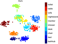
To gain a better understanding of the unsupervised representation learning capability of our proposed method, we provide a visualization of the global features of PointNet, and DGCNN backbones with OcCo [13] and our ConClu on the ModelNet10 test set in Figures 7 and 8. The features are mapped to 2D space computed using the common dimensionality reduction technique, T-SNE. Fig. 7 (a) and (b) display the embedding results of PointNet trained by OcCo [13] and our ConClu, respectively. The embeddings of “nightstand” and “dresser” are mixed together for both methods due to their strong visual similarities. Similar results can be observed from Fig. 8 (a) and (b), which show the embedding results of DGCNN trained by OcCo [13] and our ConClu, respectively. In general, our method generates more discriminative clusters than OcCo [13], which demonstrates the semantic and class separable ability of our unsupervised learning method.


IV-B2 Part segmentation
We adopt a part segmentation task to explore the per-point features obtained through our unsupervised pre-training. Part segmentation aims to assign the part category label (e.g., chair leg, cup handle) to each point for an inputted 3D point cloud. We fine-tune and evaluate the model on the ShapeNetPart [54] benchmark, which contains 16,881 objects from 16 categories and has 50 parts in total. Each object consists of 2048 points. During testing, the post-processing is the same as [8]. The overall accuracy (OA) and the mean class intersection over union (mIoU) are used as evaluative criteria to evaluate segmentation performance. Table II compares ConClu initialization with random, Jigsaw [44], and OcCo [13] initialization on object part segmentation. Our method improves the part segmentation performance and exceeds the state-of-the-art baselines (Jigsaw and OcCo) in terms of OA and mIoU. For PointNet, our pre-training improves the performance by 1.9% OA and 1.8% mIoU compared against training using random initialization (93.7% OA, 84.0% mIoU). Our ConClu initialized DGCNN backbone achieves 94.8% OA and 85.2% mIoU overall test accuracy, and it outperforms the random initialized DGCNN (92.2 OA, 84.4% mIoU) by more than 2.6% OA and 0.8% mIoU. It also slightly surpasses the second-best, OcCo initialized DGCNN (94.4% OA, 85.0% mIoU) by 0.4% OA, 0.2% mIoU. Fig. 9 visualizes the results of part segmentation initialized with our model, showing that our method can achieve a excellent performance for part segmentation.
| Encoder | Method | Accuracy | |
| OA () | mIoU () | ||
| PointNet | Random | 92.8 | 82.2 |
| Jigsaw [44] | 93.1 | 82.2 | |
| OcCo [13] | 93.4 | 83.4 | |
| Ours ConClu | 93.7 | 84.0 | |
| DGCNN | Random | 92.2 | 84.4 |
| Jigsaw [44] | 92.7 | 84.3 | |
| OcCo [13] | 94.4 | 85.0 | |
| Ours ConClu | 94.8 | 85.2 | |


IV-B3 Semantic segmentation
Semantic segmentation, a technique that associates points or voxels with semantic object labels [58], is a fundamental research challenge in point cloud processing. We use this task to evaluate the effectiveness of our method on data that goes beyond simple, free-standing objects. The pre-trained model of the semantic segmentation is fine-tuned on the Stanford Large Scale 3D Indoor Spaces (S3DIS) benchmark [59]. S3DIS consists of 3D scans collected using Matterport scanners from 6 indoor areas, containing 271 rooms and 13 semantic classes. The same pre-processing, post-processing, and training settings as [13] are adopted in our experiments. Each point is described by a 9-dimensional vector (coordinates, RGBs, and normalized location). Table III summarizes the quantitative results. The ConClu-initialized models outperform the excellent baselines Jigsaw and OcCo, in terms of OA and mIoU. PointNet and DGCNN initialized with our ConClu consistently improve their random-initialized counterpart by 4.0% to 1.3% in OA and 8.2% to 4.3% in mIoU. Fig. 10 shows the visualization results, and the predictions are very close to the ground truth.
| Encoder | Method | Accuracy | |
| OA () | mIoU () | ||
| PointNet | Random | 78.9 | 47.0 |
| Jigsaw [44] | 80.1 | 52.6 | |
| OcCo [13] | 82.0 | 54.9 | |
| ours ConClu | 82.9 | 55.2 | |
| DGCNN | Random | 83.7 | 54.9 |
| Jigsaw [44] | 84.1 | 55.6 | |
| OcCo [13] | 84.6 | 58.0 | |
| ours ConClu | 85.0 | 59.2 | |

IV-C Ablation study and analysis
IV-C1 Number of clusters
We first explore the influence of the number of clusters or partitions used in the point-level clustering block, and Table IV shows the results. It is observed that varying the number of clusters by order of magnitude (16-256) affects the performance slightly (at most 0.5 and 0.6 on NodelNet40 for PointNet and DGCNN, respectively) when they are between 32 and 128. Table IV demonstrates that the number of clusters has little influence, as long as they are “enough”. Throughout the paper, we train point-level clustering block with 64 clusters for PointNet and DGCNN as it produces a good performance. Note that 32 clusters are selected for PointNet++ in our classification task (Table I), since its final layer before max-pooling only outputs 128 point-wise features.
| Method | 16 | 32 | 48 | 64 | 72 | 96 | 128 | 256 |
| PointNet | 83.2 | 86.9 | 86.9 | 87.1 | 87.3 | 87.2 | 87.0 | 85.4 |
| DGCNN | 90.6 | 90.7 | 90.7 | 91.1 | 90.9 | 90.8 | 90.5 | 90.2 |
IV-C2 Batch size
Usually, the contrastive methods that draw negative examples from the mini-batch suffer from performance drops when their batch size is reduced. Our instance-level contrasting approach does not use negative examples, and it is thus expected to be more robust to smaller batch sizes when compared to the contrastive approaches. To empirically verify this hypothesis, SimCLR [24] is chosen as our baseline. SimCLR repulses different negative pairs, while attracting the same positive pairs. We train our instance-level contrasting and SimCLR using different batch sizes from 8 to 48. Table V tabulates the performance of both instance-level contrasting and our reproduction of SimCLR for batch sizes between 48 down to 8. The performance of SimCLR rapidly deteriorates when the batch size is 8, likely due to the decrease in the number of negative examples. By contrast, the fluctuation of performance of our approach is slight, which suggests that our method is robust to batch sizes as long as there are “enough” for batch normalization. Note that the influence of the batch size for point-level clustering is not discussed here since our clustering method is not involved in contrasting the similarity of pairs.
| Method | 8 | 16 | 24 | 32 | 40 | 48 |
| PointNet + SimCLR | 87.5 | 88.0 | 88.2 | 88.1 | 88.5 | 88.4 |
| PointNet + Ours | 88.5 | 88.3 | 88.8 | 88.7 | 88.4 | 88.6 |
| DGCNN + SimCLR | 88.6 | 89.3 | 89.4 | 89.5 | 89.7 | 90.1 |
| DGCNN + Ours | 91.0 | 91.2 | 91.1 | 91.2 | 91.3 | 91.2 |
IV-C3 Method Design Analysis
To examine the effectiveness of our designs, we also analyze PointNet and DGCNN on ModelNet40/10. Here, the projection dimension for PointNet and DGCNN is 256, and the batch size is 32. The results on ModelNet40 are summarized in Table VI (MN40). The instance-level contrasting model gets a classification accuracy of for DGCNN and for PointNet. Point-level clustering can significantly improve the accuracy of the baseline model, which increased nearly by and for PointNet and DGCNN, respectively. A similar conclusion can be drawn on ModelNet10 from Table VI (MN10). DGCNN can achieve the accuracy of 93.8%, and PointNet can achieve the accuracy of 92.4% only utilizing the instance-level contrasting. When instance-level contrasting is incorporated with point-level clustering, it can improve the performance of PointNet by 0.8% and DGCNN by 1.1%, respectively. Note that our point-level clustering-based unsupervised learning also achieves competitive results. It convincingly verifies the effectiveness of our methods.
| Model | Accuracy | |||
| MN40 | MN10 | |||
| PointNet ConClu | 88.7 | 92.4 | ||
| 87.2 | 92.3 | |||
| 89.6 | 93.2 | |||
| Model | Accuracy | |||
| MN40 | MN10 | |||
| DGCNN ConClu | 91.2 | 93.8 | ||
| 91.1 | 94.0 | |||
| 91.8 | 94.9 | |||
V Conclusion
We have proposed ConClu, a general unsupervised representation learning scheme for 3D point cloud by combining instance contrasting and points clustering to enable learning the global and local geometries. Our approach has shown promising results in transferring the pre-trained representations to various downstream 3D understanding tasks (e.g., classification, part segmentation, and semantic segmentation). Our ConClu is independent of any specific neural network architecture for point-wise classification, which allows us to use our method as a generic module for feature extraction from raw point cloud data to improve other 3D models performances.
References
- [1] M. Xu, Z. Zhou, and Y. Qiao, “Geometry sharing network for 3d point cloud classification and segmentation.,” in AAAI, pp. 12500–12507, 2020.
- [2] S. Cheng, X. Chen, X. He, Z. Liu, and X. Bai, “Pra-net: Point relation-aware network for 3d point cloud analysis,” TIP, vol. 30, pp. 4436–4448, 2021.
- [3] J. Biswas and M. Veloso, “Depth camera based indoor mobile robot localization and navigation,” in ICRA, pp. 1697–1702, 2012.
- [4] Y. Li, L. Ma, Z. Zhong, F. Liu, M. A. Chapman, D. Cao, and J. Li, “Deep learning for lidar point clouds in autonomous driving: a review,” TNNLS, 2020.
- [5] Y. Park, V. Lepetit, and W. Woo, “Multiple 3d object tracking for augmented reality,” in ISMAR, pp. 117–120, 2008.
- [6] J. Guo, J. Liu, and D. Xu, “Jointpruning: Pruning networks along multiple dimensions for efficient point cloud processing,” TCSVT, 2021.
- [7] Z. Han, Z. Liu, J. Han, C.-M. Vong, S. Bu, and C. L. P. Chen, “Mesh convolutional restricted boltzmann machines for unsupervised learning of features with structure preservation on 3-d meshes,” TNNLS, vol. 28, no. 10, pp. 2268–2281, 2016.
- [8] C. R. Qi, H. Su, et al., “Pointnet: Deep learning on point sets for 3d classification and segmentation,” in CVPR, pp. 652–660, 2017.
- [9] C. R. Qi, L. Yi, et al., “Pointnet++: Deep hierarchical feature learning on point sets in a metric space,” in NeurIPS, pp. 5099–5108, 2017.
- [10] Y. Wang, Y. Sun, Z. Liu, S. E. Sarma, M. M. Bronstein, and J. M. Solomon, “Dynamic graph cnn for learning on point clouds,” ACM TOG, vol. 38, no. 5, pp. 1–12, 2019.
- [11] A. Muzahid, W. Wanggen, F. Sohel, M. Bennamoun, L. Hou, and H. Ullah, “Progressive conditional gan-based augmentation for 3d object recognition,” Neurocomputing, vol. 460, pp. 20–30, 2021.
- [12] Y. Guo, H. Wang, Q. Hu, H. Liu, L. Liu, and M. Bennamoun, “Deep learning for 3d point clouds: A survey,” TPAMI, 2020.
- [13] H. Wang, Q. Liu, X. Yue, J. Lasenby, and M. J. Kusner, “Unsupervised point cloud pre-training via view-point occlusion, completion,” in ICCV, 2020.
- [14] W. Li, Z. Zhao, A.-A. Liu, Z. Gao, C. Yan, Z. Mao, H. Chen, and W. Nie, “Joint local correlation and global contextual information for unsupervised 3d model retrieval and classification,” TCSVT, 2021.
- [15] J.-B. Grill, F. Strub, F. Altché, C. Tallec, P. H. Richemond, E. Buchatskaya, C. Doersch, B. A. Pires, Z. D. Guo, M. G. Azar, et al., “Bootstrap your own latent: A new approach to self-supervised learning,” in NeurIPS, 2020.
- [16] Y. Yang, C. Feng, Y. Shen, and D. Tian, “Foldingnet: Point cloud auto-encoder via deep grid deformation,” in CVPR, pp. 206–215, 2018.
- [17] M. Sarmad, H. J. Lee, et al., “Rl-gan-net: A reinforcement learning agent controlled gan network for real-time point cloud shape completion,” in CVPR, pp. 5898–5907, 2019.
- [18] Y. Rao, J. Lu, and J. Zhou, “Global-local bidirectional reasoning for unsupervised representation learning of 3d point clouds,” in CVPR, 2020.
- [19] Y. Shi, M. Xu, S. Yuan, and Y. Fang, “Unsupervised deep shape descriptor with point distribution learning,” in CVPR, pp. 9353–9362, 2020.
- [20] K. Hassani and M. Haley, “Unsupervised multi-task feature learning on point clouds,” in ICCV, pp. 8160–8171, 2019.
- [21] Z. Han, X. Wang, et al., “Multi-angle point cloud-vae: unsupervised feature learning for 3d point clouds from multiple angles by joint self-reconstruction and half-to-half prediction,” in ICCV, pp. 10441–10450, 2019.
- [22] A. Sanghi, “Info3d: Representation learning on 3d objects using mutual information maximization and contrastive learning,” in ECCV, pp. 626–642, Springer, 2020.
- [23] O. Poursaeed, T. Jiang, H. Qiao, N. Xu, and V. G. Kim, “Self-supervised learning of point clouds via orientation estimation,” in 3DV, pp. 1018–1028, 2020.
- [24] T. Chen, S. Kornblith, et al., “A simple framework for contrastive learning of visual representations,” ICML, 2020.
- [25] X. Chen and K. He, “Exploring simple siamese representation learning,” in CVPR, 2021.
- [26] T. K. Moon, “The expectation-maximization algorithm,” IEEE Signal processing magazine, vol. 13, no. 6, pp. 47–60, 1996.
- [27] G. psychology, “Gestalt psychology — Wikipedia, the free encyclopedia.”
- [28] M. Zaheer, S. Kottur, et al., “Deep sets,” in NeurIPS, pp. 3391–3401, 2017.
- [29] Y. Li, R. Bu, et al., “Pointcnn: Convolution on x-transformed points,” in NeurIPS, pp. 820–830, 2018.
- [30] W. Wu, Z. Qi, and L. Fuxin, “Pointconv: Deep convolutional networks on 3d point clouds,” in CVPR, pp. 9621–9630, 2019.
- [31] Y. Liu, B. Fan, et al., “Relation-shape convolutional neural network for point cloud analysis,” in CVPR, pp. 8895–8904, 2019.
- [32] M. Xu, R. Ding, H. Zhao, and X. Qi, “Paconv: Position adaptive convolution with dynamic kernel assembling on point clouds,” in CVPR, 2021.
- [33] H. Zhou, Y. Feng, M. Fang, M. Wei, J. Qin, and T. Lu, “Adaptive graph convolution for point cloud analysis,” in CVPR, pp. 4965–4974, 2021.
- [34] T. Sun, G. Liu, R. Li, S. Liu, S. Zhu, and B. Zeng, “Quadratic terms based point-to-surface 3d representation for deep learning of point cloud,” TCSVT, 2021.
- [35] D. Ding, C. Qiu, F. Liu, and Z. Pan, “Point cloud upsampling via perturbation learning,” TCSVT, vol. 31, no. 12, pp. 4661–4672, 2021.
- [36] F. Song, Y. Shao, W. Gao, H. Wang, and T. Li, “Layer-wise geometry aggregation framework for lossless lidar point cloud compression,” TCSVT, 2021.
- [37] L. Zhao, J. Guo, D. Xu, and L. Sheng, “Transformer3d-det: Improving 3d object detection by vote refinement,” TCSVT, 2021.
- [38] S. Huang, Y. Xie, S.-C. Zhu, and Y. Zhu, “Spatio-temporal self-supervised representation learning for 3d point clouds,” in ICCV, 2021.
- [39] B. Eckart, W. Yuan, C. Liu, and J. Kautz, “Self-supervised learning on 3d point clouds by learning discrete generative models,” in CVPR, pp. 8248–8257, 2021.
- [40] X. Liu, Z. Han, et al., “L2g auto-encoder: Understanding point clouds by local-to-global reconstruction with hierarchical self-attention,” in ACM MM, pp. 989–997, 2019.
- [41] S. Chen, C. Duan, Y. Yang, D. Li, C. Feng, and D. Tian, “Deep unsupervised learning of 3d point clouds via graph topology inference and filtering,” TIP, vol. 29, pp. 3183–3198, 2019.
- [42] P. Achlioptas, O. Diamanti, I. Mitliagkas, and L. Guibas, “Learning representations and generative models for 3d point clouds,” in ICML, pp. 40–49, PMLR, 2018.
- [43] X. Gao, W. Hu, and G.-J. Qi, “Graphter: Unsupervised learning of graph transformation equivariant representations via auto-encoding node-wise transformations,” in CVPR, pp. 7163–7172, 2020.
- [44] J. Sauder and B. Sievers, “Self-supervised deep learning on point clouds by reconstructing space,” in NeurIPS, pp. 12942–12952, 2019.
- [45] S. Xie, J. Gu, D. Guo, C. R. Qi, L. Guibas, and O. Litany, “Pointcontrast: Unsupervised pre-training for 3d point cloud understanding,” in ECCV, pp. 574–591, Springer, 2020.
- [46] J. Bromley, I. Guyon, Y. LeCun, E. Säckinger, and R. Shah, “Signature verification using a” siamese” time delay neural network,” NeurIPS, vol. 6, pp. 737–744, 1993.
- [47] X. Xu and G. H. Lee, “Weakly supervised semantic point cloud segmentation: Towards 10x fewer labels,” in CVPR, pp. 13706–13715, 2020.
- [48] B. Xu, N. Wang, T. Chen, and M. Li, “Empirical evaluation of rectified activations in convolutional network,” arXiv preprint arXiv:1505.00853, 2015.
- [49] M. Cuturi, “Sinkhorn distances: Lightspeed computation of optimal transport,” NeurIPS, vol. 26, pp. 2292–2300, 2013.
- [50] G. Peyré, M. Cuturi, et al., “Computational optimal transport: With applications to data science,” Foundations and Trends® in Machine Learning, vol. 11, no. 5-6, pp. 355–607, 2019.
- [51] A. Paszke, S. Gross, et al., “Pytorch: An imperative style, high-performance deep learning library,” in NeurIPS, pp. 8024–8035, 2019.
- [52] S. Gugger and J. Howard, “Adamw and super-convergence is now the fastest way to train neural nets,” last accessed, vol. 19, 2018.
- [53] A. Sharma, O. Grau, and M. Fritz, “Vconv-dae: Deep volumetric shape learning without object labels,” in ECCV, pp. 236–250, 2016.
- [54] L. Yi, V. G. Kim, D. Ceylan, I.-C. Shen, M. Yan, H. Su, C. Lu, Q. Huang, A. Sheffer, and L. Guibas, “A scalable active framework for region annotation in 3d shape collections,” ACM TOG, vol. 35, no. 6, pp. 1–12, 2016.
- [55] S. Liu, L. Giles, and A. Ororbia, “Learning a hierarchical latent-variable model of 3d shapes,” in 3DV, pp. 542–551, IEEE, 2018.
- [56] M. Gadelha, R. Wang, et al., “Multiresolution tree networks for 3d point cloud processing,” in ECCV, pp. 103–118, 2018.
- [57] L. Zhang and Z. Zhu, “Unsupervised feature learning for point cloud understanding by contrasting and clustering using graph convolutional neural networks,” in 3DV, pp. 395–404, IEEE, 2019.
- [58] Z. Song, L. Zhao, and J. Zhou, “Learning hybrid semantic affinity for point cloud segmentation,” TCSVT, 2021.
- [59] I. Armeni, O. Sener, A. R. Zamir, H. Jiang, I. Brilakis, M. Fischer, and S. Savarese, “3d semantic parsing of large-scale indoor spaces,” in CVPR, pp. 1534–1543, 2016.