Unsupervised learning of topological phase transitions using the Calinski-Harabaz index
Abstract
Machine learning methods have been recently applied to learning phases of matter and transitions between them. Of particular interest is the topological phase transition, such as in the XY model, whose critical points can be difficult to be obtained by using unsupervised learning such as the principal component analysis. Recently, authors of [Nature Physics 15,790 (2019)] employed the diffusion map method for identifying topological orders and were able to determine the Berezinskii-Kosterlitz-Thouless (BKT) phase transition of the XY model, specifically via the intersection of the average cluster distance and the within-cluster dispersion parameter (when the different clusters vary from separation to mixing together). However, sometimes it is not easy to find the intersection if or does not change too much due to topological constraint. In this work, we propose to use the Calinski-Harabaz () index, defined roughly as the ratio , to determine the critical points, at which the index reaches a maximum or minimum value, or jumps sharply.
We examine the index in several statistical models, including ones that contain a BKT phase transition. For the Ising model, the peaks of the quantity or its components are consistent with the position of the specific heat maximum. For the XY model, both on the square and honeycomb lattices, our results of the index show the convergence of the peaks over a range of the parameters in the Gaussian kernel.
We also examine the generalized XY model with and and study the phase transition using the fractional -vortex or -vortex constraint respectively. The global phase diagram can be obtained by our method, which does not use the label of configuration needed by supervised learning, nor a crossing from two curves and . Our method is thus useful to both topological and non-topological phase transitions and can achieve accuracy as good as supervised learning methods previously used in these models, and may be used for searching phases from experimental data.
pacs:
05.70.Fh, 64.60.ah, 64.60.De,64.60.at,89.20.FfI introduction
Exploring phases of matter and phase transitions is a traditional but still active research direction in statistical physics pt ; qpt , partly due to new phases of matter that have been uncovered. In recent years, this field of research is revived thanks to the introduction of artificial intelligence and machine learning methods to recognize phases and transitions roger1 . Among the various methods, supervised learning methods are used to train the network using prior labeled data generated by Monte Carlo methods in various classical systems, such as the Ising model and its variants roger1 ; longising ; smising , XY models hu ; mlpxy ; rogerxy ; Wessel with BKT phase transitions xykt ; bkt , Dzyaloshinskii-Moriya ferromagnets dm , skyrmions sky , Potts models Potts and percolation models mlpxy . The properties of quantum systems, such as the energy spectrum, entanglement spectrum confu1 , or configuration in the imaginary time fermi ; xuefeng are also used as inputs to the neural networks for the training. On the other hand, unsupervised learning methods can provide unbiased classification, as they do not need prior knowledge of the system so as to classify phases and obtain the phase transition. These include methods such as the principal component analysis wang1 , autoencoders unp , t-SNE unsup1 , clustering with quantum mechanics tony . A key feature of these is to determine the sought-after properties (such as phase transition) by examining indicators from the scattered plot in the reduced space. Beyond equilibrium statistical physics, non-equilibrium and dynamical properties dy ; nonequi2 ; out2 are also obtained by machine learning methods. In addition, there are other newly developed schemes applied to the phases of matter, such as the adversarial neural networks adv , confusion method and its extension dcn , the super resolving method rs , and even applications to experimental data ex1 ; ex2 . Other developments in this area can be found in Refs. topo-inv ; z2spin ; tp2 ; mbl ; jgliu ; ml ; selfmap ; tool ; spinor ; conf ; order ; exp and the review article rev .
It is well known that in traditional continuous phase transitions global symmetry is broken and these transitions can be described by the Landau theory. However, the topological phase transitions have no broken symmetry and therefore it is of great interest to understand how the transitions emerge and how to locate the transition points. Recent developments of machine learning offers new tools for this endeavor hu ; rogerxy ; Wessel ; mlpxy , based on supervised learning. However, the learning-by-confusion scheme when applied to the XY model predicts a transition temperature set by the value located at the maximum of the specific heat Wessel . In Ref. rogerxy , it was found that significant feature engineering of the raw spin states is needed to relate vortex configurations and the transition. Moreover, a single-hidden-layer Fully Connected Networks (FCN) could not correctly learn the phases in the XY model, whereas the Convolutional Neural Networks (CNN) was successfully employed to learn the BKT transition rogerxy , and the classification was later extended to the generalized XY model mlpxy . However, for unsupervised learning with the PCA method, it was claimed to be difficult to identify the transition hu . Recently, Rodriguez-Nieva and Scheurer used the diffusion map method nature invented by R.R. Coifman and S. Lafon lafon and related to quantum clustering tony , and devised an unsupervised learning method for identifying topological orders and successfully locating the BKT transition. They divided the configurations into several topological sectors with different winding numbers, then calculated the eigenvector and eigenvalues of the so-called diffusion matrix (see Sec. II.1). From the intersections of the average cluster distance and within-cluster dispersion , or equivalently the intersection of (the jump in the eigenvalues) and (the standard deviation of the eigenvalues), the phase transition of the XY model on the square lattice can be obtained very well.
Our motivation of this study is to examine whether or not the diffusion map (DM) method of Rodriguez-Nieva and Scheurer (RNS method) is suitable beyond the pure XY model, such as the generalized XY model. Indeed we find that the DM method works for some topological phase transitions, but it fails to locate the phase transition in the generalized XY model in other regimes. Specifically, the RNS method for determining the transition point relies on the intersection of the two curves (such as the average cluster distance and within-cluster dispersion ), and in the generalized XY model, as illustrated in Sec. V, we cannot find an intersection there. The thermal fluctuation is not strong enough and the scattering clusters with different winding as numbers do not mix close to , i.e. does not decrease substantially. The question arises: are there other quantities that can be used to locate the phase transition points?
In this work, we mainly use the Calinski-Harabaz (ch) index score CH defined by , related to the ratio of , which means that if the variation of can be negligible due to strong topological constraints, the variation of itself can help to determine the phase transition point. We also use the Silhouette coefficient () lunkuo or its components to compare with the results.
The outline of this work is as follows. Sec. II shows the DM methods, the definition of the indices , and their components, their advantage and prior knowledge for using the indices. Sec. III shows the signature of and for the two-dimensional Ising model from configurations using the Swendsen-Wang algorithms SW . In Sec. IV, the critical phase transition points of the XY model on the square and the honeycomb lattices are obtained using the DM method. In Sec. V, for the and generalized XY models, the global phase diagrams are obtained by the DM method assisted by PCA or k-PCA methods. Other techniques are discussed in Sec. VI regarding the effect of higher dimensions considered in the k-means method and how to automatically find the hyperparameter . Concluding comments are made in Sec.VII. In Appendix A, the simplest example 1D XY model is discussed, and the comparison between PCA and k-PCA is shown in Appendix B. Finally, a total of 11 indices used in unsupervised learning are listed in Appendix C.
II Methods
II.1 The review of diffusion map method
Here, we explain the DM method of Rodriguez-Nieva and Scheurer nature . Assume that we have configurations , where . The connectivity between and is denoted by the elementary Gaussian kernel
| (1) |
The normalization of can be done by performing the sum over ,
| (2) |
We can also perform the normalization along the direction of (i.e., the sum over ). The eigenvalue equation of the diffusion matrix is , where ’s are the right eigenvectors, with the corresponding eigenvalues , for .
To find the phase transition point, Ref. nature and its earlier preprint version prep use two different ways, respectively:
(a)
Intersection of the mean distance of cluster centers , where is the number of clusters, and the dispersion of the data
points in each cluster. The quantities and are obtained from the scatter plot, where is the number of topological sectors.
After obtaining the eigenvectors of the matrix given by
| (3) |
the authors project them unto a two-dimensional space, namely, a two-column matrix, then and the dispersion
can be
obtained from the scatter plot of the two column vectors or their modified version. The detailed application to
the one-dimensional XY model is reproduced in Appendix A.
(b) Intersection of the mean fluctuation and gap of eigenvalues , where
| (4) |
and the gap of eigenvalues between the topological sectors and ,
| (5) |
II.2 The indices ch and sc
We propose to use indices instead of intersections. Based on the first two leading eigenvectors and of the PCA, kernel-PCA (kPCA) or the second and third vectors and of the DM method, for a manually chosen cluster numbers , the index is given in terms of the following ratio:
| (6) |
where is the between-group dispersion matrix and is the within-cluster dispersion matrix and they are defined as follows,
| (7) |
where is the number of data points, is the set of points in cluster , is the center of cluster , and denotes the average center of all cluster centers , and the number of points in cluster . The index of the -th sample is
| (8) |
where is the mean distance between sample and all other data points in the same cluster, is the mean dissimilarity of point to some cluster expressed as the mean of the distance from to all points in (where ). The mean over all points of a cluster is a measure of how tightly grouped all the points in the cluster are. Sometimes or are also very useful 11index .
The performance of a total of 11 indices is shown in Appendix C and the results of indices , , and applied to the generalized XY model are all reasonable choices. Here, we choose two representative indices and as examples.

II.3 Advantage and prior knowledge required using ch
Fig. 1 draws the flowchart of the RNS method and the place of our modifications. Depending on whether or not we are considering topology, we perform dimensional reduction by DM or PCA (k-PCA) respectively, to get the features of the data, i.e., the eigenvectors of the diffusion matrix or the covariance matrix. Then we apply k-means to cluster the two-dimensional or higher dimensional scattering points. If we do not choose “ch”, then intersections of and , or intersections of and nature ; prep can be used instead.
To test whether the clustering is good or bad, if “” is chosen, then the peaks of or its components and will be used directly. For the topological phase transition, the index or its component and can give signatures of phase transition when it is not easy to determine the intersection of the RNS method or when there is no intersection.
The index can also be applied to non-topological phase transitions, such as the order-disorder phase transition of the Ising model. This does not require any prior knowledge except for the configurations generated by e.g. Monte Carlo methods or from real experiments.
For topological phase transitions, such as the XY and generalized XY models, although this type of unsupervised learning is not similar to supervised learning (such as fully-connected layers, or convolutional neural networks), it still needs labels of configurations, i.e., the topological winding number and the number of possible phases. However, the label of the topological winding number does not mean the label of phases, and essentially, this method is still an unsupervised learning method.
III The 2D Ising model
To test the ability to locate the phase transition point , we calculate for the simplest model, i.e., the Ising model,
| (9) |
where is the ferromagnetic interaction between a pair of nearest neighborhood spins, and . The unsupervised learning of Ising model has been studied before, (see e.g., Refs. wang1 ; unp ).
We use a two-dimensional lattice and generate samples for each temperature and analyze them by PCA, using the scattering data of the first two leading eigenvectors and . Moreover, we calculate () and sc() for each according to Eqs. (6) and (8).
Figure 2 shows the main results for the Ising model. In Fig. 2 (a), itself and have a sharp decrease whereas has peaks around (here we re-scale the results so the maximum value is 1). In Figs. 2 (b) and (c), the index is peaked around ; and also have a sharp jump at the phase transition points.
To understand these results, the scatter plot of and are shown in Figs. 2 (d)-(f) for temperatures , 2.3 and 2.9, respectively. At low temperature, the clusters identified by the two colors separate from each other in the reduced space and finally mix together at high temperatures.
In general, the index is large when the clusters are well separated and the points in each cluster are well aggregated. From this viewpoint, in the low temperature phase, the index becomes large because all up states and all down states can be easily distinguished if the analysis is successful.
The index and their components perform well in detecting the transition, and the position of the peak or the jump is the largest at . Around the phase transition point, configurations possess the properties from both phases (paramagnetic and ferromagnetic) and the fluctuation is the largest there.
Comparing to traditional Monte Carlo results with the same size as shown in Fig.2 (g)-(i), we find that the position of the peak is located at around 2.295 consistent with our or results with numerical intervals of 0.01. For the purpose of reference, the thermodynamic limit transition is marked.


It should be noted that if we simulate the Ising model by the Metropolis Monte Carlo algorithm metro , which flips one spin each time, in the low temperature limit, almost all spins choose to sit in the initial state (i.e., , spin up). The scatter plot will simply have one group. However, this is not wrong because the state still obeys the Boltzmann distribution. This is the reason of small at low temperatures of using the Metropolis algorithm to generate configurations. However, we can still observe the signature at the phase transition point. Using the Swendsen-Wang algorithm instead SW , i.e., a global updating Monte Carlo method, the spin states will all be spin up or spin down in lower temperatures, which is not dependent of the initial state.
IV The 2D XY model
The Hamiltonian of the classical XY model is given by
where denotes a nearest-neighbor pair of sites and , and in is a classical variable defined at each site describing the angles of spin directions in a two-dimensional spin plane. The sum in the Hamiltonian is over nearest-neighbor pairs on the square lattice with the periodic boundary condition; other lattices can be also considered.
IV.1 The 2D XY model on square lattices
Now we analyze the first example, i.e., the two-dimensional XY model on the square lattice. Firstly, we generate the configurations with five fixed winding number pairs at , , , and . For each fixed winding number pair, it should be noted that, for the two-dimensional geometry, the winding number component means that the spins in each row form a winding number of rather than just the spins on one row randomly selected. Cluster simulation algorithms wf ; SW are not suitable to update the spins because the global flips break the topological winding number easily and therefore the Metropolis algorithm is used while trying to rotate the spin vector with a very small step each time so as to preserve the winding number.
For each topological sector, we generate configurations. Combining all configurations from all five sectors, we construct the kernel . The elements between is defined in Eq. (1) and the normalized matrix is obtained, obeying its eigenvalue equation . Using the scatter plot of the second and third leading eigenvectors and of , the index are obtained and displayed in Figs. 3 (a)- (d).
There is a parameter in the above matrices and in order to deduce consistent results, we need to make sure the results are converging for a finite range of . We see that this is indeed the case for different values of in Figs. 3(a)-(d). For , , & , is less than , and then becomes when , , , , and . Finally, the peaks move left and deviate from again when or larger. It should be noted that here, or more Monte Carlo steps, are used in order to reach the equilibrium of systems.
The estimated points are labeled by the circles in Fig. 3 (e) and they all distribute nearby or on the red lines representing the latest result critical temperature kao The intersections of and are labeled by the gray regions in the critical regimes from Ref. nature . It appears that it is easier to use to locate the phase transition as we only need to identify the peak location. The results from Ref. nature have greater uncertainty than those by using the index.
The histogram of our estimated is shown in Fig. 3 (f), which helps to determine the hyperparameter (see Sec. VI).


In Fig. 3 (g)-(i), the finite size effect of is checked using the with two smaller sizes and with , & . Combining the estimated with , we use two different ways of (linear, exponential) extrapolation to get in the thermodynamic limit. The results are and , respectively.
IV.2 2D XY model on honeycomb lattices
Here, we study the second example , i.e., the pure XY model on the honeycomb lattice, as the critical point is known exactly at 0.7 .
The geometry of the honeycomb lattice is equivalent to the brick-wall lattice shown in Fig. 4, where every spin has three nearest-neighbor spins. To initialize the configurations with a fixed winding number (, )=(0, 1), the spins connected by solid gray lines are defined as forming in the vertical direction. Specifically, if we start a spin at position (2,1), and then go left to (1,1) (1,2) (2,8) and go back to (2,1) through the red dashed lines, connecting the sites at the boundaries for periodic boundary conditions, the spins sweep an angle of counter-clockwise.
It should be noted that two spins, such as (1,1) and (2,1), connected by the horizontal gray lines will contribute to the winding number , and they also contribute to . This poses a problem when fixing and independently. Fortunately, this problem can be solved. Specifically, in the first row, labeled by 1 in the vertical () direction, the relation of angles obeys . During the simulation, small fluctuations are allowed if they do not break the winding number.

In Fig. 5, using configurations constrained in five topological sectors on the lattices, we find that the peaks are located at the exact value for several different values of in the interval [2,6] with intervals of 0.5. We also calculate the intersections by and at 5, 6, 7. The intersection can also arrive at when , but not 5 and 6. It indicates that the performs better than the intersection as the intersection method may not give a high confidence of the transition.


V 2D Generalized XY (GXY) models
Here, we apply our method to the generalized XY models q8mc ; q2mc , whose Hamiltonian is given by
where is the relative weight of the pure model, and is another integer parameter that can drive the system to form a nematic phase. For both and the model reduces to the pure XY model (redefining as in the first case), and hence the transition temperature is identical to that of the pure XY model. However, such a redefinition is not possible with . The phase diagrams of the GXY models depend on the integer parameter , and they have been explored extensively.
V.1 q=2 GXY model
The GXY model has a richer phase diagram than the XY model and has an additional new phase mlpxy . Thus, it is a good candidate model to test our method away from the pure XY limit. The phase diagram is illustrated in Fig. 6 (a) on the plane, and we also show the results from our unsupervised method and those from PCA as comparison. The symbols , , represent nematic, ferromagnetic and paramagnetic phases, respectively. The dashed lines are data from the MC simulations q2mc mainly of up to . The color indicates the value of index obtained from simulation with the system size . We now discuss the -, - and - transitions as follows.
(i) The - phase transition: Interestingly, the positions of the peaks by are consistent with the dashed line of the phase boundary in the whole region . The index performs very well where is away from the pure XY model limit. The essential nature of the - phase transition is still BKT.
(ii) The - phase transition: In the regime , the peaks around , which is less than . This discrepancy is likely due to the nature of half-vorticity in the phase. We can improve the result by limiting the configurations to have the half-winding number as the topological constraint in our Monte Carlo simulation. The half-vortex physics has been discussed in Ref. q2mc .
Thus, we only consider (,) in the four types of combinations (, 0) and (0, ). To form (,0), the difference between a pair of spins located at the left most and right most boundaries is fixed as and we assign each spin using the Eq. (14). With the half vortex constraint, our results illustrated by the red symbols move closer to the dashed lines of the transition in Fig. 6 (a) than the results using the integer-value constraint.
Figs. 6 (b) and (c) show the details at and , respectively. For , we generate two groups of data and the peaks almost converge in the interval , and the convergence is closer to than the result from the integer vortex constraint. For , the half vortex constraint gives better results at .
(iii) The - phase transition: When we realize that the topological constraint makes the peaks (features) of the distribution for the spin directions implicit in the and phases, we use the configurations without any constraint in this case. The results are labeled by purple symbols with legend ‘, ’.
The behavior of depends on the structure of the sample points, and sometimes emerges as a sharp jump at the phase transition point such as in the Ising model discussed in the main text. Sometimes it is a local minimum value at the phase transition point. Take the GXY model at as an example, in Fig. 7, both and increase as a function of . However the difference decreases first and then increases around , where the gap has a positive value.

According to the following equation:
| (10) |
clearly, and the local minimum of the is at the location of .

For the - phase transition in Fig. 6 (a), the PCA is stronger than the DM method. Here, we would like to give a physical discussion about this because such a difference is related to the advantage of the proposed method, and thus a more detailed discussion should be made.
The reasons for PCA being stronger for the transition can be explained as follows:
(i) The phase transition is not a topological phase transitionq8mc . The DM method designed here is to determine the topological phase transition. It is still interesting to see the of DM by inputting Ising configurations without any topological constraint. In Fig. 9, using k-PCA and the DM method with complete same configurations, the signatures of phase transition emerge and the results are consistent at . However, the signature of k-PCA method is clearer.
(ii) From the view of the data, it is also understandable that PCA is stronger. Without any topological constraint, in the nematic () phase, the spins prefer two dominant directions and their histograms obey a double peaks structure. In the Ferromagnetic () phase, one main direction remains and one peak emerges for the histograms. Fig. 8 (b1)-(b3) show the typical histograms in three phases. The main feature difference between the phases is obvious.
However, with a topological constraint, the spin directions are mainly distributed according to the winding numbers. For example, the spin angles in each row are
with additional fluctuations,
where and are the number index and total number, respectively, in each row.
Therefore, the distribution sits almost in the range as shown in
Figs. 8(a1)-(a3).
The feature difference of spin angles disappears when using the constraint.
Therefore, the DM method cannot get transition points using the configurations with constraints.


V.2 q=8 GXY model
For the GXY model q8mc , Fig. 10 (a) shows the global phase diagram using the values of the index. The phases , , , are obtained and the distributions are also shown.
In the new phase, the distribution of the spin vectors has 8 peaks, but is dominated by possible angles. The ‘X’ shape dashed lines are from Refs. q2mc ; q8mc . The orange color represents the values of by the DM method.
Let us first discuss the ()- transition. Clearly, for - transition in the range , the peak positions of align well with the dashed line. In the center of ’X’, the and transition are also consistent with MC result i.e., .
However, we could not use the intersection of the cluster average distance and within-cluster dispersion as described in Ref. nature because does not vary too much and there is no intersection as shown in Figs. 10 (e)-(g). The five different colors therein represent the five typical topological sectors. However, fortunately, when zooming in the figures in Figs. 10 (g)-(i), we find that, near the transition region, the shape of a fixed cluster shrinks because the data points gather closer together, and hence the within-cluster dispersion is smaller. The index thus develops a peak around as shown in Fig. 10 (c), with and also displayed in Fig. 10 (d). In contrast, Fig. 10 (b) shows that cannot be used to signal the transition temperature because it evaluates the difference, , but in spite of the fact that has a local minimum.
It should be mentioned that for the - transition, the use of either the integer or half vortex constraint is not suitable. Instead the vortex constraint is needed in generating the configurations. Moreover, after comparison, we find that kPCA works better if we use as the input into the kPCA (using PCA does not work well). The kernel used for kPCA defined as a radial basis functional kernel , where is the system size, and are the configurations and is the default value gp .
The other details of the -, -, - and - transitions will be discussed as follows.

For the GXY model, Figs. 11 show the distributions of spin vectors in the (a1) , (a2) and (a3) phases with the integer-vortex constraint. The distributions of spin vectors in the and phase have no obvious differences. To distinguish the and phases, the constraints are canceled and the distributions are shown in Figs. 11 (b1)-(b3) respectively.

Figs. 12 (a)-(d) show the detail of phase transition -, -, -, respectively. For the - transition, in Fig. 12 (a), fixing in the interval at steps of , the peaks of are located at and respectively, completely matching the dashed lines in the global phase diagram in Fig.10.
In Fig. 12 (b), for the - transition, by fixing , the peaks of are located at with , , , and . The other values of are not shown. In Fig. 12 (c), fixing =, and , the positions of local minimum of located at , and respectively.
In Fig.12 (d), for , using the vortex constraint results in the most accurate critical points. The peak position is at more closely to than by the integer vortex constraint. The error bars are obtained by the bootstrap method using 400 randomly chosen configurations between the total 2000 configurations and total of 20 bins.
VI Other technical modifications
In the above sections, during the use of the k-means method, we apply two output eigenvectors of the diffusion matrix and then get the values of the index. The conclusion is that using two leading vectors leads to the best accuracy. At the same time, it is possible to design a way to determine the super parameter automatically. In this section, we will focus on such issues for the completeness of our method.

Here, the effects of higher-dimensional features will be discussed using k-means, namely, whether or not the accuracy is enhanced when including more features will be clarified. The answer is that retaining more dimensions of the eigenvectors, the result may deviate from the right critical points or even predict wrong critical points.
Assuming the covariance matrix of the PCA method is , and its eigenvectors are , where . For the Ising model, in Sec. III, the first and second vectors , are used, where , or . Here, we consider vectors with , and . The difference is found between the results of two-dimensional vectors and higher dimensional data, as shown in Figs. 13(a)-(c). The estimated position of peaks are , and respectively. The result for is the closest to the peak of the specific heat.
For the generalized XY model (, ), with the DM method, the vectors with index () are used
as the first vector ignored.
In Fig.13 (d), with or ,
the position of peaks are as the same as that of
. However, if higher-dimensional data are used, such as and ,
the score does not yield the correct signature of the phase transition
as shown in Figs.13 (e) and (f).
Another issue discussed here is whether one can design an automatic method to determine the hyperparameter . Since its value has been tried many times for some reasonable choices, one may expect to find a way to determine its optimal value automatically.
To the best of our knowledge, at present, there are no such automatic determination of the hyperparameter . Here we devise a simple analysis from the statistics (histogram) of obtained by various :
-
i.
Calculate as a function of temperature with various in a range from to by using the configurations with topological constraints;
-
ii.
Store the position of peaks, i.e., and the times they appear as shown in Fig. 3 (e) and (f). Sometimes, the peaks may not be not obvious, and a plateau emerges. The two ends of the plateau will be stored.
The histogram of vs. can be used to give the best estimate for the transition. Therefore, corresponding to the highest position , the values
are acceptable.
Another possible approach is to calculate a location dependent for each data point instead of selecting a single scaling parameter localsigma . Then, the kernel matrix between a pair of points can be written as
| (11) |
where and are the local scale parameters for and , respectively. The selection of the local scale is determined by the local statistics of the neighborhood of point . For example, the scale can be set as
| (12) |
where is the -th nearest neighbor. However, here, K is also a hyperparameter to be chosen. By comparing Eq. (11) and Eq. (1), , the obtained is about several times larger than the acceptable regimes.
VII Discussion and Conclusion
In summary, we use the Calinski-Harabaz () index to successfully locate phase transitions of a few classical statistical models, including the Ising, XY and the generalized XY models. From the scatter data, for which we use the index to obtain the phase transitions for the Ising, XY and GXY models on lattices. This combines the advantages of the PCA and DM methods, as the scattering data can be based on either the first two leading eigenvectors of the PCA Kernel-PCA or the second and third vectors from DM method.
The advantages of using the index are less steps, wider applications and better convergence. After k-means applied to the eigenvectors of the diffusion matrix , using the index, we do not need to maximize the visibility of cluster as proposed in RNS method. For some phase transitions, it may not be easy to find the intersections of and . In Figs. 10 (e)-(g), index could capture the signatures of both quantities. In Fig. 5, for the pure XY model on the honeycomb lattices, the exact critical point is at . Using , when is in the interval [2,6], the estimated results of are all close to .
In the pure XY limit, we have tested that can locate the phase transition for the XY model on both the square and honeycomb lattices, similar to the DM method of Rodriguez-Nieva and Scheurer. For the GXY model, the values of the index in the whole phase diagram matched the boundary between the ferromagnetic phase to paramagnetic phase very well even away from the pure XY limit. Close to the - transition, the accuracy can be improved by using the -vortex constraint in generating the Monte Carlo configurations. For the GXY model, using intersections of and cannot be used to locate the transition point, such as at , but the index can still work to locate the phase transition point due to its incorporation of the fluctuation of samples within each cluster. Moreover, the - transition can also be identified by using the vortex constraint.
We have also compared the results from other indices (see Table 1), but we find that the index works best overall for the models considered in this work. In the future, it will be desirable to systematically study the utility of various parameters in models of statistical physics that exhibit different natures of transitions.
The development of applying machine learning to physics could develop new methods for studying unknown phases. For the Ising model or similar models, the transition point is well known. This situation will help to check our proposed method.
If we get the first-hand data from experiments, and do not know the details of the Hamiltonian, our unsupervised method can help deduce the number of possible classes (phases) in the data. Furthermore, using the index we could identify phase transition points. Therefore, the method of using the index is very useful for future non-topological phase transitions. For the XY model and Hamiltonians similar to the GXY model, by using the index, topological phase transition points were obtained without using the traditional method of measuring correlations q8mc and spin stiffness kao . Of course, some reasonable prior knowledge is needed such as the possible winding numbers. The idea of DM can be applied to topological quantum systems (see Refs. band ; dff ). In principle, the topological quantum phases and transitions between them may be probed using the or indices.
Acknowledgements.
We thank for the valuable discussion with J. F. Rodriguez-Nieva, M. S. Scheurer, Y. Z. You and T. Chotibut on simulations. We also thank Tony C Scott for his help. TCW is supported by the National Science Foundation under Grant No. PHY 1915165 J. Wang and H. Tian are supported by NSFC under Grant No. 51901152. W. Zhang is supported from Science Foundation for Youths of Shanxi Province under Grant No. 201901D211082;References
- (1) H. E. Stanley, Introduction to Phase Transitions and Critical Phenomena (Oxford University Press, New York, 1971).
- (2) S. Sachdev, Quantum Phase Transitions, (Cambridge University Press, UK, 1999).
- (3) J. Carrasquilla and R. Melko, Machine learning phases of matter, Nat. Phys. 13, 431 (2017).
- (4) K. I. Aoki, T. Kobayashi, Restricted Boltzmann Machines for the Long Range Ising Models, Mod. Phys. Lett. B 30, 1651401 (2016).
- (5) D. Kim and D. Kim, Smallest neural network to learn the Ising criticality, Phys. Rev. E 98, 022138 (2018).
- (6) W. Hu, R. R. P. Singh, and R. T. Scalettar, Discovering phases, phase transitions, and crossovers through unsupervised machine learning: A critical examination, Phys. Rev. E 95, 062122 (2017).
- (7) M. Beach, A. Golubeva and R. Melko, Machine learning vortices at the Kosterlitz-Thouless transition, Phys. Rev. B 97, 045207 (2018).
- (8) P. Suchsland and S. Wessel, Parameter diagnostics of phases and phase transition learning by neural networks, Phys. Rev. B 97, 174435 (2018).
- (9) W. Zhang, J. Liu and T.-C. Wei, Machine learning of phase transitions in the percolation and XY models, Phys. Rev. E 99, 032142 (2019).
- (10) Kosterlitz, J. M. Thouless and D. J. Ordering, metastability and phase transitions in two-dimensional systems, J. Phys. C 6, 1181 (1973).
- (11) Berezinskii, V. Destruction of long-range order in one-dimensional and two-dimensional systems possessing a continuous symmetry group. II. Quantum systems, Sov. J. Exp. Theor. Phys. 34, 610 (1972).
- (12) V. Singh and J. Han, Application of machine learning to two-dimensional Dzyaloshinskii-Moriya ferromagnets, Phys. Rev. B 99, 174426, (2019).
- (13) I. A. Iakovlev, O. M. Sotnikov and V. V. Mazurenko Supervised learning approach for recognizing magnetic skyrmion phases, Phys. Rev. B 98, 174411 (2018).
- (14) C. Li, D. Tan and F. Jiang, Applications of neural networks to the studies of phase transitions of two-dimensional Potts models, Ann. Phys. 391, 312 (2018).
- (15) E. van Nieuwenburg, Y. Liu and S. Huber, Learning phase transitions by confusion, Nat. Phys. 13, 435 (2017).
- (16) P. Broecker, J. Carrasquilla, R. Melko and S. Trebst, Machine learning quantum phases of matter beyond the fermion sign problem, Sci. Rep. 7 8823 (2017).
- (17) X. Dong, F. Pollmann and X. Zhang, Machine learning of quantum phase transitions, Phys. Rev. B 99, 121104 (2018).
- (18) L. Wang, Discovering Phase Transitions with Unsupervised Learning, Phys. Rev. B 94, 195105, (2016).
- (19) S. J. Wetzel, Unsupervised learning of phase transitions: From principal component analysis to variational autoencoders, Phys. Rev. E 96, 022140 (2017).
- (20) K. Ch’ng, N. Vazquez and E. Khatami, Unsupervised machine learning account of magnetic transitions in the Hubbard model, Phys. Rev. E 97, 13306 (2018).
- (21) T. C. Scott, M. Therani, and X. M. Wang, Data Clustering with Quantum Mechanics, Mathematics, 5, 5 (2017).
- (22) E. van Nieuwenburg, E. Bairey and G. Refael, Learning phase transitions from dynamics, Phys. Rev. B 98, 060301 (2018).
- (23) J. Venderley, V. Khemani and E. Kim, Machine learning out-of-equilibrium phases of matter, Phys. Rev. Lett. 120, 257204 (2018).
- (24) C. Casert, T. Vieijra, J. Nys and J. Ryckebusch, Interpretable machine learning for inferring the phase boundaries in a nonequilibrium system, Phys. Rev. E 99, 023304 (2019).
- (25) P. Huembeli, A. Dauphin and P. Wittek, Identifying quantum phase transitions with adversarial neural networks, Phys. Rev. B 97, 134109 (2018).
- (26) Y. Liu and E. P. L. van Nieuwenburg, Discriminative Cooperative Networks for Detecting Phase Transitions, Phys. Rev. Lett. 120, 176401 (2018).
- (27) S. Efthymiou, M. J. S. Beach, and R. G. Melko, Super-resolving the Ising model with convolutional neural networks, Phys. Rev. B 99, 075113 (2019).
- (28) W. Lian et al. Machine Learning Topological Phases with a Solid-State Quantum Simulator, Phys. Rev. Lett. 122, 210503 (2019).
- (29) A. Bohrdt et al., Classifying snapshots of the doped Hubbard model with machine learning, Nat. Phys. 15, 921 (2019).
- (30) P. Zhang, H. Shen and H. Zhai, Machine Learning Topological Invariants with Neural Networks, Phys. Rev. Lett. 120, 066401 (2017).
- (31) Y. Zhang, R. Melko and E. Kim, Machine learning Z2 quantum spin liquids with quasiparticle statistics, Phys. Rev. B 96, 245119 (2017).
- (32) Y. Zhang and E. A. Kim, Quantum Loop Topography for Machine Learning, Phys. Rev. Lett. 118, 216401 (2017).
- (33) Y. Hsu, X. Li, D. Deng and S. Das Sarma, Machine Learning Many-Body Localization: Search for the Elusive Nonergodic Metal, Phys. Rev. Lett. 121, 245701 (2018).
- (34) Z. Cai and J. Liu Approximating quantum many-body wave functions using artificial neural networks, Phys. Rev. B 97,035116 (2018).
- (35) R. Vargas-Hernández, J. Sous, M. Berciu and R. Krems, Extrapolating Quantum Observables with Machine Learning: Inferring Multiple Phase Transitions from Properties of a Single Phase, Phys. Rev. Lett. 121, 255702 (2018).
- (36) A. Shirinyan, V. Kozin, J. Hellsvik and M. Pereiro, Self-organizing maps as a method for detecting phase transitions and phase identification, Phys. Rev. B 99, 041108 (2019).
- (37) C. Giannetti, B. Lucini and D. Vadacchino, Machine Learning as a universal tool for quantitative investigations of phase transitions, Nucl. Phys. 944 114639 (2019).
- (38) J. Greitemann, K. Liu and L. Pollet Probing hidden spin order with interpretable machine learning, Phys. Rev. B 99, 060404 (2019)
- (39) S. S. Lee and B. J. Kim, Confusion scheme in machine learning detects double phase transitions and quasi-long-range order, Phys. Rev. E 99, 043308 (2019).
- (40) P. Ponte and R. G. Melko, Kernel methods for interpretable machine learning of order parameters, Phys. Rev. B 96, 205146 (2017).
- (41) Z. Li, M. Luo, and X. Wan, Extracting critical exponents by finite-size scaling with convolutional neural networks, Phys. Rev. B 99, 075418 (2019).
- (42) Giuseppe Carleo et al., Machine learning and the physical sciences, Rev. Mod. Phys. 91, 045002 (2019).
- (43) J. F. Rodriguez-Nieva and M. S. Scheurer, Identifying topological order through unsupervised machine learning, Nat. Phys. 15, 790 (2019).
- (44) R. R Coifman, S. Lafon, A. B. Lee, M. Maggioni, B. Nadler, F. Warner, S.W. Zucker. Geometric diffusions as a tool for harmonic analysis and structure definition of data: Diffusion maps, PNAS. 102 (21), 7426(2005).
- (45) T. Caliński and J. Harabasz, A dendrite method for cluster analysis, Commun. Stat. - Theory Methods 3, (1974).
- (46) P. J. Rousseeuw, Silhouettes: a graphical aid to the interpretation and validation of cluster analysis, J. Comput. Appl. Math. 20, 53 (1987).
- (47) R. H. Swendsen, J. S. Wang, Nonuniversal critical dynamics in Monte Carlo simulations, Phys. Rev. Lett. 58 86 (1987).
- (48) J. F. Rodriguez-Nieva and M. S. Scheurer, arXiv:1805.05961v1.
- (49) Y. Liu, Z. Li, H. Xiong, X. Gao, J. Wu and S. Wu, Understanding and Enhancement of Internal Clustering Validation Measures, in IEEE Transactions on Cybernetics, 43, 3, (2013).
- (50) N. Metropolis, A.W. Rosenbluth, M.N. Rosenbluth, A.H. Teller, E. Teller, Equation of State Calculations by Fast Computing Machines, J. Chem. Phys. 21 1087 (1953).
- (51) U. Wolff, Collective Monte Carlo Updating for Spin Systems, Phys. Rev. Lett. 62, 361 (1989).
- (52) Y. Hsieh, Y. J. Kao and A. W. Sandvik. Finite-size scaling method for the Berezinskii-Kosterlitz-Thouless transition, J Stat. Mech-Theory 2013, P09001 (2013).
- (53) B. Nienhuis, Exact Critical Point and Critical Exponents of O() Models in Two Dimensions, Phys. Rev. Lett. 49, 1062 (1982); Y. Deng, T. Garoni, W. Guo, H. Blöte and A. Sokal, Cluster simulations of loop models on two- dimensional lattices, Phys. Rev. Lett. 98, 120601 (2007).
- (54) D. M. Hübscher and S. Wessel, Stiffness jump in the generalized XY model on the square lattice, Phys. Rev. E 87, 062112 (2013).
- (55) G. A. Canova, Y. Levin, and J. J. Arenzon, Competing nematic interactions in a generalized XY model in two and three dimensions, Phys. Rev. E 94, 032140 (2016).
- (56) F. Pedregosa, G. Varoquaux, A. Gramfort et. al., Scikit-learn: Machine Learning in Python, Journal of Machine Learning Research, 12, 2825 (2011).
- (57) L. Zelnik-Manor and P. Perona, Self-Tuning Spectral Clustering, Neural Inf. Process. Syst. 17 1601 (2004); G. Mishne and I. Cohen, Multiscale Anomaly Detection Using DFs, IEEE Journal of Selected Topics in Signal Processing (JSTSP), 7, 111 (2013).
- (58) M. S. Scheurer and Robert-Jan Slager, Unsupervised machine learning and band topology, Phys. Rev. Lett. 124, 226401 (2020).
- (59) Y. Long, J. Ren and H. Chen, Unsupervised Manifold Clustering of Topological Phononics, Phys. Rev. Lett. 124, 185501 (2020).
Appendix A The 1D XY model
The Hamiltonian of the pure XY model reads
| (13) |
where is the coupling strength of the nearest neighboring pair of spins and throughout this work, we set for simplicity and use the periodic boundary condition . For simplicity, following Ref. nature , we generate the spin vectors according to the following,
| (14) |
where is the winding number, is the identification number of the configuration {}, with varying from 1 to the total length . The first term is used to define the winding number , where the is in the range by the so-called saw function rogerxy obtained by replacing with if it is not in the target range. The term obeys the Gaussian fluctuation and is generated randomly between [0, ).
We consider two types of generated configurations with winding numbers and . The histogram of the values of the first component of the diffusion map is shown in Fig. 14 (a). The histogram of has values at and is a vector with size , therefore the values are equal to when is re-scaled by . Fig. 14 (b) shows the largest 20 eigenvalues of the transition probability matrix in Eq. (2). Two maximum eigenvalues are found equal to unity. Following Ref. nature , we also test according to the following equation,
| (15) |
where . We find that has seven district values ranging from to , corresponding to seven winding numbers marked by the symbols in Fig. 14 (c). Eigenvalues vs. is also shown in Fig. 14 (d). Clearly, the plateau of eigenvalues appears in .


Figs. 15 (a)-(c) show the largest 24 eigenvalues of as a function of for , 0.6 and 1.0, respectively. The band of eigenvalues could not be distinguished for small values of and the reason can be seen from the matrix of , which is a diagonal matrix in that limit. Increasing , the band of will separate away from each other.
The choice of is important. We choose marked by the dashed lines in the left column. The right column presents versus (). Clearly, the gap between the eigenvalue and eigenvalue becomes smaller when increasing temperature and subsequently disappears when .
Appendix B The PCA and K-PCA


Figs. 16, represent some results of PCA and kPCA on simple and generalized datasets in the appendix of Ref. nature .
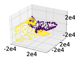
The simple datasets are configurations of one-dimensional XY model with size , , and and with topological winding numbers and according to Eq. (14). Figure 16 show results of linear PCA, PCA with Gaussian kernels, and PCA with polynomial kernels, respectively (the top left, top middle and top right panels). Obviously, the classifications of PCA with a nonlinear kernel are much more clear for the XY models. The three dimensional visualization is based on the three reduced components. However, the above method fails for data generated with slight modification of Eq. (14) with an additional term , where is random in the range [, ]. The results are shown in Fig. 16 at the bottom left, bottom middle and bottom right panels, respectively.
Appendix C Other indices
As listed in Ref. 11index , we check the 11 indices listed in Table (1) for validating the classifications. Take the GXY model as an example, the value of the parameters such as the temperature and are fixed as those in Fig. 10 (b). We find only four indices, presented in Fig.17 (a)-(d) produce signals at the critical points. These are , , and , whose full names are listed in Table (1).
The other indices could not give correct signals to locate the phase transition points.

| measure | Notation | Definiton | ||||||
|---|---|---|---|---|---|---|---|---|
| 1 | Calinski-Harabasz index | |||||||
| 2 | Silhouette index |
|
||||||
| 3 | Davies-Bouldin index | |||||||
| 4 | SDbw validity index |
|
||||||
| 5 | Xie-Beni index | |||||||
| 6 | Dunn’s indices | |||||||
| 7 | pbm | |||||||
| 8 | I index | |||||||
| 9 | Root-mean-square std dev | |||||||
| 10 | R-squared | |||||||
| 11 | Modified Hubert statistic |
-
1
: dataset ; : number of objects in ; : center of ; : attributes number of ; : number of clusters ; : the i-th cluster; : number of objects in ; : center of ; : variance vector of ; : distance between and ; .