Unsupervised Learning of Hybrid Latent Dynamics:
A Learn-to-Identify Framework
Abstract
Modern applications increasingly require unsupervised learning of latent dynamics from high-dimensional time-series. This presents a significant challenge of identifiability: many abstract latent representations may reconstruct observations, yet do they guarantee an adequate identification of the governing dynamics? This paper investigates this challenge from two angles: the use of physics inductive bias specific to the data being modeled, and a learn-to-identify strategy that separates forecasting objectives from the data used for the identification. We combine these two strategies in a novel framework for unsupervised meta-learning of hybrid latent dynamics (Meta-HyLaD) with: 1) a latent dynamic function that hybridize known mathematical expressions of prior physics with neural functions describing its unknown errors, and 2) a meta-learning formulation to learn to separately identify both components of the hybrid dynamics. Through extensive experiments on five physics and one biomedical systems, we provide strong evidence for the benefits of Meta-HyLaD to integrate rich prior knowledge while identifying their gap to observed data.
1 Introduction
Learning the dynamics underlying observed time-series is at the heart of many applications, such as health monitoring and autonomous driving. As the quality and diversity of observation data continue to improve, modern applications increasingly require deep learning capabilities to extract latent dynamics from high-dimensional observations (e.g., images), without label access to the latent variables being modeled. This unsupervised learning of latent dynamics presents a fundamental challenge of identifiability that is distinct from supervised modeling at the data space: different latent abstraction may be learned to reconstruct an observed time-series, but do they all guarantee an adequate identification of the governing dynamic functions?
Recent works have shown that integrating inductive bias, in the form of known physics-based dynamic functions at the latent space, enables identification of the latent state variables and even parameters of the dynamic function with simple unsupervised objectives of data reconstruction, as illustrated in Fig. 1A [35, 25, 17]. These approaches however require the physics of the latent dynamic function to be accurately known, which is not always possible in practice.
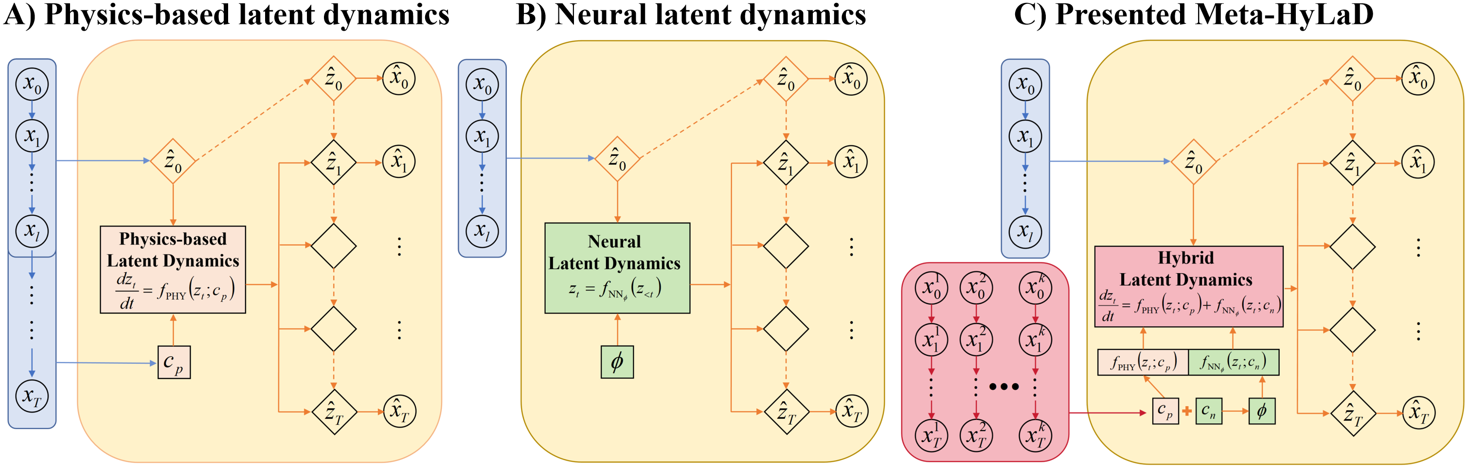
This limitation has been recognized in emerging hybrid models that combines physics-based dynamic functions with neural networks describing potentially unknown components in the prior physics [16, 38, 10, 13, 29]. The existing hybrid models, however, are all learned at the data space with direct supervision on the state variables being modeled by the dynamic function. There are no existing solutions supporting unsupervised learning of hybrid dynamic functions at the latent space.
In this paper, we investigate the identifiability of neural latent dynamic functions and show that – unlike physics-based functions – a neural latent dynamic function without physics inductive bias cannot be adequately identified with an unsupervised reconstruction objective. Indeed, there has been a variety of purely neural-network based latent dynamic models which, as illustrated in 1B, are learned with an unsupervised forecasting objective to use several initial frames to predict a longer sequence [32, 1, 2]. These latent dynamic functions, however, are optimized globally for the entire training data: i.e., the training process results in the identification of a single dynamic function without retraining. Adopted directly in hybrid latent dynamics, this will result in a strong assumption that the gap between the prior physics and observed data are globally shared across all samples. This challenge may be further aggravated when the physics-based and neural components – both heterogeneous across samples – need to be separately identified.
To this end, we introduce the first solution to unsupervised learning of hybrid latent dynamics (Meta-HyLaD). As illustrated in Fig. 1C, in contrast to existing purely physics-based or neural approaches (Fig. 1A-B), Meta-HyLaD has two key innovations. First, inspired by [29], we formulate the latent dynamic function in the form of a universal differential equation (UDE), , where describes prior physics specific to the data under study and is a neural network describing potential errors in the prior physics, each with parameter and to be identified. Second, we present a novel learn-to-identify solution where, instead of learning/identifying a single that can only describe a gloal discrepancy between and the true governing dynamics, we train feedforward meta-models to learn to identify : we will show that this strategy – asking latent dynamic functions to forecast for samples different from those used to identify them – is critical to their successful identifications.
We evaluate Meta-HyLaD on a spectrum of dynamic systems ranging from relatively simple benchmark physics to tracer kinetics underlying dynamic positron emission tomography (PET) imaging [27]. We first demonstrate that the unsupervised reconstruction objectives cannot guarantee the adequate identification of a neural latent dynamic function, and that this can be overcome either by the incorporation of a physics-based dynamic function or – at the absence of such physics inductive bias – the presented learn-to-identify formulation (Section 4.2). We then demonstrate the clear improvements in system identification and time-series forecasting obtained by Meta-HyLaD in comparison to purely physics-based, purely neural, or hybrid models with a global neural component (Section 4.3). Finally, we demonstrate the advantages of Meta-HyLaD in comparison to a wide variety of existing works – both physics- and neural-based latent dynamic models and their extensions to meta-learning formulations – across different types of errors in the prior physics and across the datasets considered (Section 4.4). The results provide strong evidence for the benefits of hybrid dynamics to integrate rich prior knowledge while allowing for their errors, as well as the importance of properly identifying these hybrid components.
2 Related Works
Unsupervised learning of latent dynamics: There has been a surge of interests in learning the governing dynamics of high-dimensional time-series, mostly in an encoder/decoder formulation with the goal to identify a dynamic function and its resulting state variables at the latent space.
Physics-based (white-box) latent dynamics: Several methods have proposed to integrate physics-based dynamic equations into the latent space as prior knowledge specific to the data under study [35, 25, 17]. They however require the physics of the latent dynamics to be accurately known (with only some physics parameters unknown), which is not always possible in practice. We will show that – at the presence of different types of errors in the prior physics – the performance of this type of white-box modeling quickly deteriorates. How to leverage physics-based functions while addressing their errors remains an open question in learning latent dynamics.
Neural (black-box) latent dynamics: There has also been an explosion of neural-network based latent dynamic models, using for instance LSTMs [4, 23, 8, 19] and neural ODEs [36, 2] at the latent space. Different from white-box dynamic functions with physically-meaningful latent state variables and parameters, black-box dynamic functions are associated with abstract latent states and functions. It thus sees an increased challenge of identifiability, especially when learning across heterogeneous dynamics. Among recent efforts, there has been a growing body of works exploring ways to effectively identify different neural dynamic functions from heterogeneous data samples [37, 33, 21, 18], among which meta-learning has emerged to be a promising solution [21, 18].
All of these existing works, however, are based on black-box dynamic functions without the ability to leverage potentially valuable prior knowledge. Some recent works, such as Hamiltonian and Lagrangian neural network [24, 12, 6, 11, 39, 32, 14, 28, 40, 30, 3] encode physical laws as priors to constrain the behavior of the neural latent dynamic function, blurring the boundary between black- and white-box modeling. The latent dynamic functions, however, are still in the form of neural networks. Furthermore, these approaches encompass broader priors rather than richer knowledge specific to the problem/data.
Meta-HyLaD represents the first hybrid solution to learning latent dynamics. Moreover, we dive deep into the identifiability of physics-based versus neural components, and show that – for latent dynamic functions without physics inductive bias – successful reconstruction of observed time-series does not guarantee a successful identification: a non-trivial challenge inadequately discussed in the literature.
Hybrid (grey-box) dynamics: When the dynamic function is directly supervised, a number of hybrid models has emerged to combine physics-based functions with neural networks to compensate for unknown components in the known physics. Most approaches [16, 38, 10] use a neural function to describe the residual between the simulated and the measured states. NeuralSim [13] takes it a step further and includes neural functions as different components within a physics-based function. UDEs define a differential equation with known mathematical expressions combined with neural networks [29].
These hybrid models, however, are learned at the data space and directly supervised by measured state variables of the dynamics. The absence of such supervision substantially increases the difficulty to identify the dynamic function, and Meta-HyLaD represents the first step towards a solution.
3 Methods
Fig. 1C outlines the key elements in Meta-HyLaD: 1) hybrid latent dynamic functions, and 2) learn-to-identify strategies.
3.1 Hybrid Latent Dynamic Functions as a UDE
Considering high-dimensional time-series , we model its generation process as:
| (1) |
where function describes the latent dynamics of the state variables , and function describes the emission of the latent state variables to the observed data.
Latent dynamic functions: While Meta-HyLaD is agnostic to the type of dynamic functions used in Equation (1), we choose an ordinary differential equation (ODE) to describe the latent dynamics as a continuous process that can be emitted to the observation space only when needed. More specifically, we describe the latent dynamics as a UDE:
| (2) |
where represents the known physics equation governing the data, and its unknown parameters. represents the potential errors in the prior physics, modeled by a neural network with weight parameters . Instead of identifying a single neural function that will only model a global discrepancy between and the true governing dynamics, we further allow it to change with a parameter that can be identified from data: more specifically, we use to generate the weight parameter of via a hyper network .
Emission functions: The emission function , i.e., the decoder, bridges the mapping from the latent state space to the observed data space. In most existing works considering latent physics-based functions, it has been considered critical for this emission function to be physics-based [25, 17]. Similarly, when the latent dynamic function is purely neural, it is customary to adopt a neural function as the emission function [2]. As a secondary objective of this paper, we will investigate the use of a physics-based vs. neural decoder for different types of latent dynamic functions. We denote them generally as where is known if is physics-based, and unknown if is a neural network parameterized with .
3.2 Learn-to-Identify via Meta-Learning
Given an observed time-series in training data , a common approach to identifying its latent dynamic process is to infer its time-varying latent state to reconstruct [23, 19, 8, 35]. We will show that – for neural functions with abstract latent states – this reconstruction does not guarantee a correct identification of the dynamic function governing : an evidence is when the identified dynamic function, given different initial conditions, could not generate the correct time series governed by the same dynamics.
We propose that a proper identification of the latent dynamic functions requires us to go a step further: one must further separate into two key ingredients generating it – the initial latent state that is specific to the time-series sample, and parameters for the governing latent dynamic function. In a neural network where the learned functions can be arbitrary and the latent states abstract without direct supervision, this separation is not trivial. Below, we describe our learning strategies to facilitate this separation, and discuss how such identification strategies may be different for the physics-based versus neural functions.
Identifying initial latent states: The initial latent state of an observed time series is specific to that series and can be simply identified from the first several frames of observations , where :
| (3) |
where is a neural encoder with weight parameters .
Identifying latent dynamics:
To identify and for Equation (2), a simple reconstruction objective would be:
| (4) |
| (5) |
| (6) |
where and if is neural. is neural encoder parameterized by . We refer to this as a reconstruction objective, as illustrated in Fig. 2A. Although commonly used, we will show that this learning strategy – while deceivingly able to provide good reconstruction performance on a given time series – will not be able to separately identify the three components of the latent dynamic function.
Identifying the neural component: Instead of the reconstruction of an observed time-series, we present a novel learn-to-identify solution to address the identifiability challenge associated with the neural component of the latent dynamic function. The fundamental intuition is that, to separately identify time-varying latent states from time-invariant governing dynamic functions, one can leverage the statistical strength that the governing latent dynamics might be shared across multiple samples. Therefore, we can attempt to learn to identify for from one or more samples, and ask the identified function to be applicable for disjoint samples sharing the same dynamics. This is the basis for the presented learn-to-identify framework.
Formally, we cast this into a meta-learning formulation. Consider a dataset of high-dimensional time-series with similar but distinct underlying dynamics: . For each , we consider disjoint few-shot context time-series samples and query samples where . Instead of the reconstruction objective in Equations (4-6), we formulate a meta-objective to learn to identify from -shot context time-series samples , such that the identified hybrid dynamic function is able to forecast for any query time series in given only an estimate of its initial state . More specifically, we have a feedforward meta-model to learn to identify for dynamics as:
| (7) |
where an embedding is extracted from each individual context time-series via a meta-encoder and gets aggregated across to extract knowledge shared by the set. is the size of the context set, and its value can be fixed or variable which we will demonstrate in the ablation study.
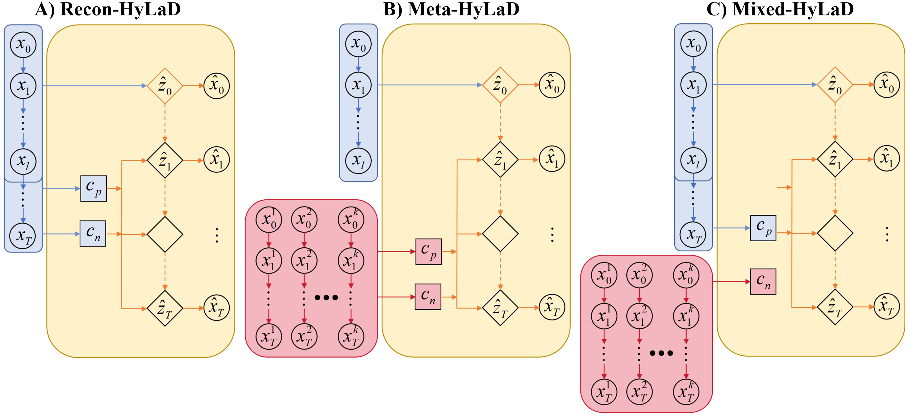
Identifying the physics-component: The parameter for the physics-based of the latent dynamic functions can be inferred in a similar fashion. However, as the structural form of the function defines specific physics meaning for the latent state variable , we will show that this physics inductive bias alone allows it to be identified with a simple reconstruction objective similar to Equations (4-6). In another word, for the physics-based dynamic function can be identified in two alternative formulations:
| Fig. 2B | (8) | ||||
| Fig. 2C | (9) |
| DataSet | Physics | Equation | Configurantion | DataSize |
| Pendulum | Full | ID OOD | 15390 | |
| Partial | ||||
| Mass Spring | Full | ID OOD | 12960 | |
| Partial | ||||
| Bouncing Ball | Full | ID OOD | 21060 | |
| Partial | ||||
| Rigid Body | ID OOD | 4800 | ||
| Full | ||||
| Partial | ||||
| Double Pendulum | Full | ID OOD | 12705 | |
| Partial | ||||
| Dynamic PET | Full | See Appendix E | 2000 | |
| Partial |
Learn-to-identify meta-objectives: Given data with different dynamics , for all query samples , we have its initial latent state identified from its own initial frames (Equation (3)), and its hybrid latent dynamic functions identified with and as described in Equations (7-8) (Fig. 2B, Meta-HyLaD), or in Equations (7) and (9) (Fig. 2C, Mixed-HyLaD). Given the inferred , and , we minimize the forecasting accuracy on the query time-series with and if is neural:
| (10) |
4 Experiments and Results
We first investigate the two key contributions of Meta-HyLaD: 1) its identification strategy in comparison to reconstruction objectives in addressing the identifiability of physics-based vs. neural latent dynamic functions (Section 4.2), and 2) its modeling strategy vs. purely physics-based, purely neural, or hybrid models with a global neural component (Section 4.3). We then evaluate Meta-HyLaD with a variety of existing physics-based and neural latent dynamic models [35, 2] along with their extensions into the presented meta-learning frameworks, considering both physics-based and neural decoders (Section 4.4). Finally, we test its feasibility on identifying radiotracer kinetics in dynamic PET (Section 4.5). All experiments are repeated with three random seeds.
| Recontruction Task | Prediction Task | |||||||
|---|---|---|---|---|---|---|---|---|
| () | () | () | () | |||||
| A – Recon-HyLaD | 3.95(0.27) | 4.34(0.74) | 2.05(0.31) | 1.13(0.26) | 7.17(0.50) | 10.59(1.06) | 1.83(0.15) | 3.72(0.69) |
| B – Meta-HyLaD (k=1) | 4.39(0.19) | 5.19(0.85) | 1.70(0.10) | 1.16(0.18) | 4.40(0.37) | 6.70(1.31) | 1.46(0.13) | 2.23(0.28) |
| C – Mixed-HyLaD (k=1) | 3.95(0.58) | 4.15(0.97) | 1.70(0.07) | 0.45(0.06) | 4.11(0.58) | 6.85(2.48) | 1.54(0.50) | 0.44(0.06) |
| B – Meta-HyLaD (k=7) | / | / | / | / | 2.86(0.13) | 2.05(0.09) | 0.28(0.00) | 0.45(0.05) |
| C – Mixed-HyLaD (k=7) | / | / | / | / | 2.62(0.11) | 1.93(0.12) | 0.32(0.07) | 0.39(0.12) |
4.1 Data & Experimental Settings
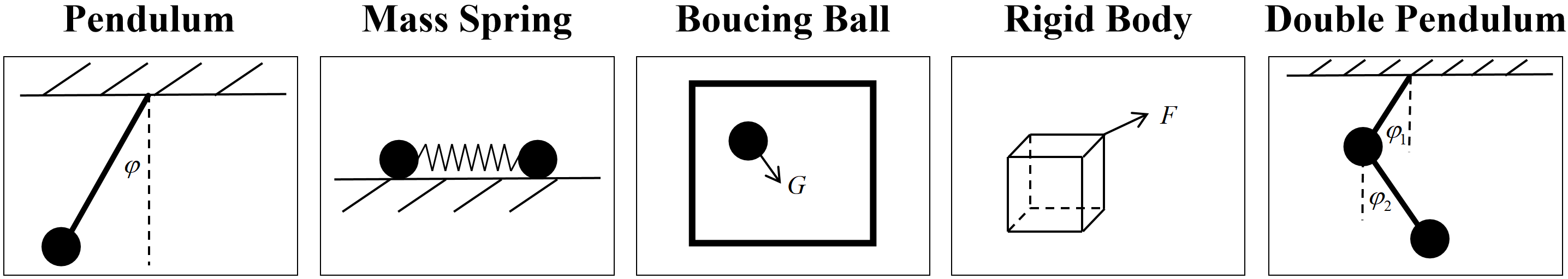
We consider common benchmarks including three simple physics systems of Pendulum [2], Mass Spring [8], and Bouncing Ball (under gravity) [2], and two more complex physics systems of Double Pendulum [2] and Rigid Rody [25]. To demonstrate feasibility towards more complex systems, we further consider an additional dataset of dynamic PET [27]. For each of the five physics system, we randomly sample the initial states and parameters of the governing dynamic function, and generate time-series of system states and the corresponding image observations by physical rendering in [25]. We refer to the dynamic functions used for the generation of data as full physics functions, and design partial physics functions to represent our imperfect prior knowledge about the observed data reflecting a variety of potentially additive and multiplicative errors as summarized in Table 1: in Pendulum and Mass Spring, partial physics lacks the knowledge about damping (additive error), in Bouncing Ball and Rigid Body, partial physics only considers gravity/force in one direction/plane (multiplicative error); in Double Pendulum, partial physics ignores the impact of the mass difference between two pendulums (multiplicative error).
To introduce heterogeneity in the underlying dynamics, in data generation we vary the parameters of the full physics equations in the components both present (blue) and absent (red) in the prior physics, with their training and test distributions and number of samples summarized in Table 1. More details on each dataset are in Appendix A. We leave descriptions of the dynamic PET dataset in Section 4.5.
4.2 Identifiability of Physics. vs. Neural Dynamics
We first evaluate the reconstruction vs. learn-to-identify objectives for identifying physics-based vs. neural latent dynamic functions, on the Pendulum dataset (see Table 1).
Models: Here we consider the three identification schemes for learning hybrid latent dynamic functions as described in Section 3.2 (Fig. 2). All three learning strategies share the same backbone architectures, with their architectural and implementation details provided in appendix G. We consider and for learn-to-identify strategies, to assess potential impact associated with the number of samples used to identify the dynamic functions.
Metrics: A successfully-identified latent dynamic function should be able to forecast a time series that is different from those used to identify it (but shares the same dynamics). To this end, we test the three learning strategies for two tasks: 1) a reconstruction task to identify and from a test time-series and reconstruct the seires itself, and 2) a prediction task where and are identified from a test time-series but used to predict another time-series that follows the same dynamics but different initial conditions.
For both tasks, we measured the mean squared error (MSE) between the ground-truth and estimated time series at both the observation and the state variable level . In addition, we consider two metrics to separately evaluate how well and are each identified: for , we directly measure the MSE between its identified and ground-truth value; for , because we do not expect its value to be physically meaningful, we instead measure the fit between the identified neural dynamic function and the ground truth residual function by their MSE.
Results: As summarized in Table 2, all three learning strategies results in strong performance to reconstruct the same time series used to identify the latent dynamic functions. However, latent dynamic functions identified with the reconstruction objective (A) fail when attempting to predict different time series sharing the same dynamics. A deeper dive reveals something interesting: the physics component () is well identified by all identification strategies (A-C); in contrast, is only successfully identified by the learn-to-identify strategy (B-C). Moreover, the mixed identification strategy (C) seems to facilitate a better identification of when , although both Meta- (B) and Mixed-HyLaD (C) achieve similar performance when is increased to 7. Interestingly, increasing for identifying also improves the identification of in Mixed-HyLaD (C). We provide visual examples of identified in appendix B.
These experiments provide two important insights: 1) a good reconstruction is not sufficient evidence that the underlying latent dynamics is correctly identified, and 2) the inclusion of physics inductive bias or the learn-to-identify strategy are two effective solutions to address the issue of identifiability.
4.3 Benefits of Hybrid Dynamic Functions
We now evaluate the benefits of hybrid latent dynamic functions on the five physics systems described in Section 4.1.
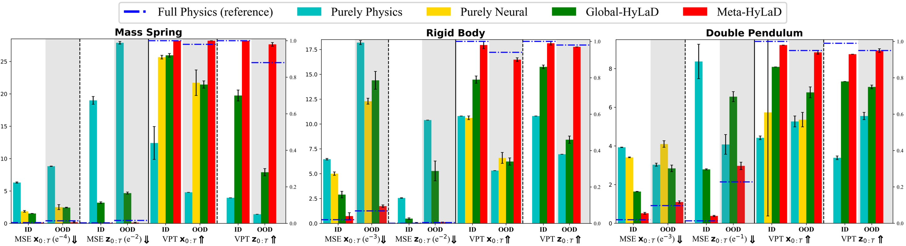
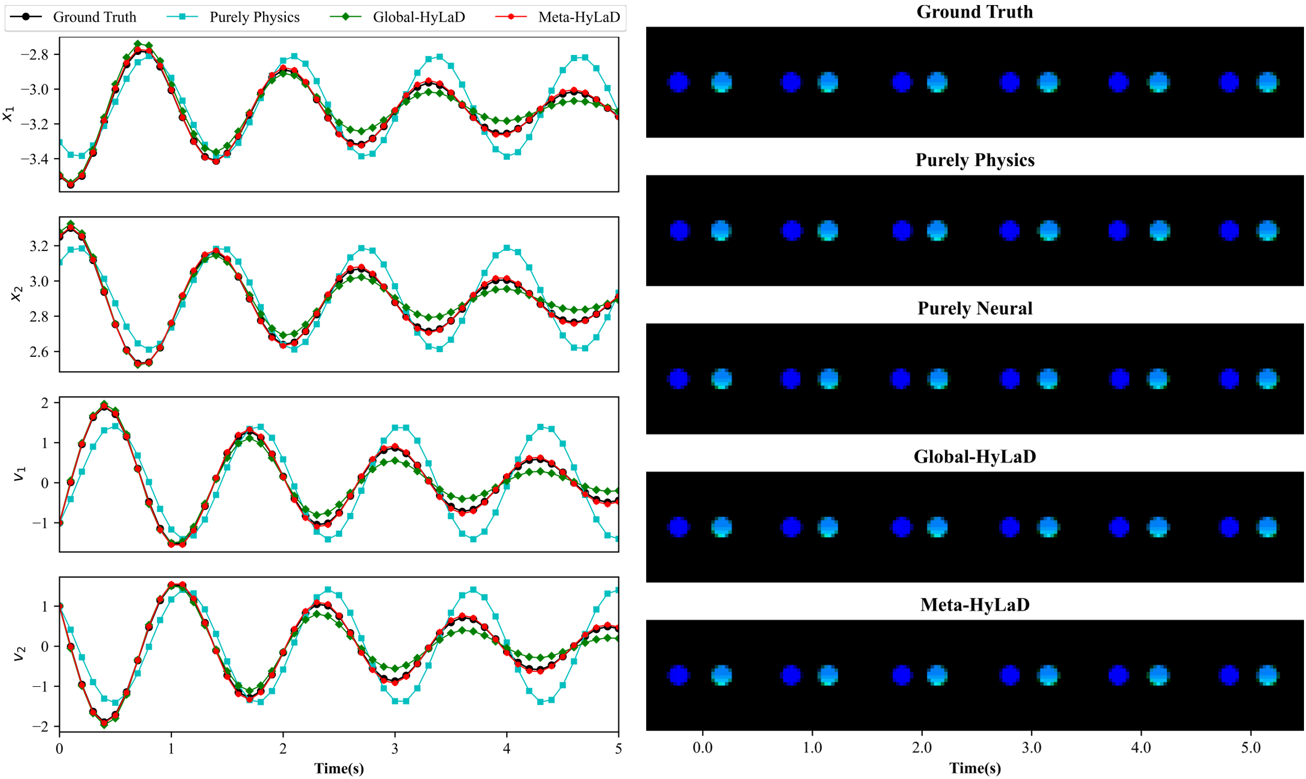
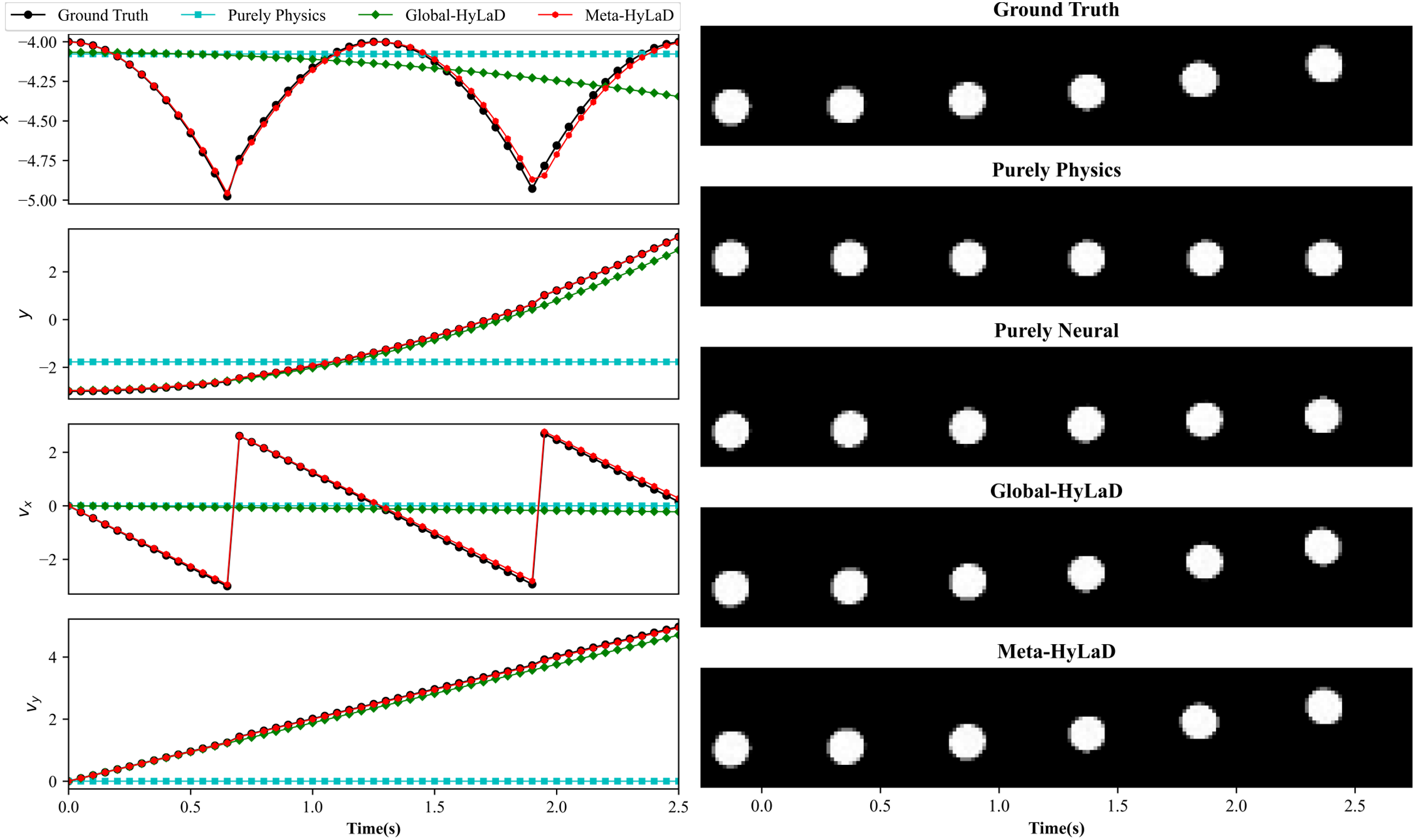
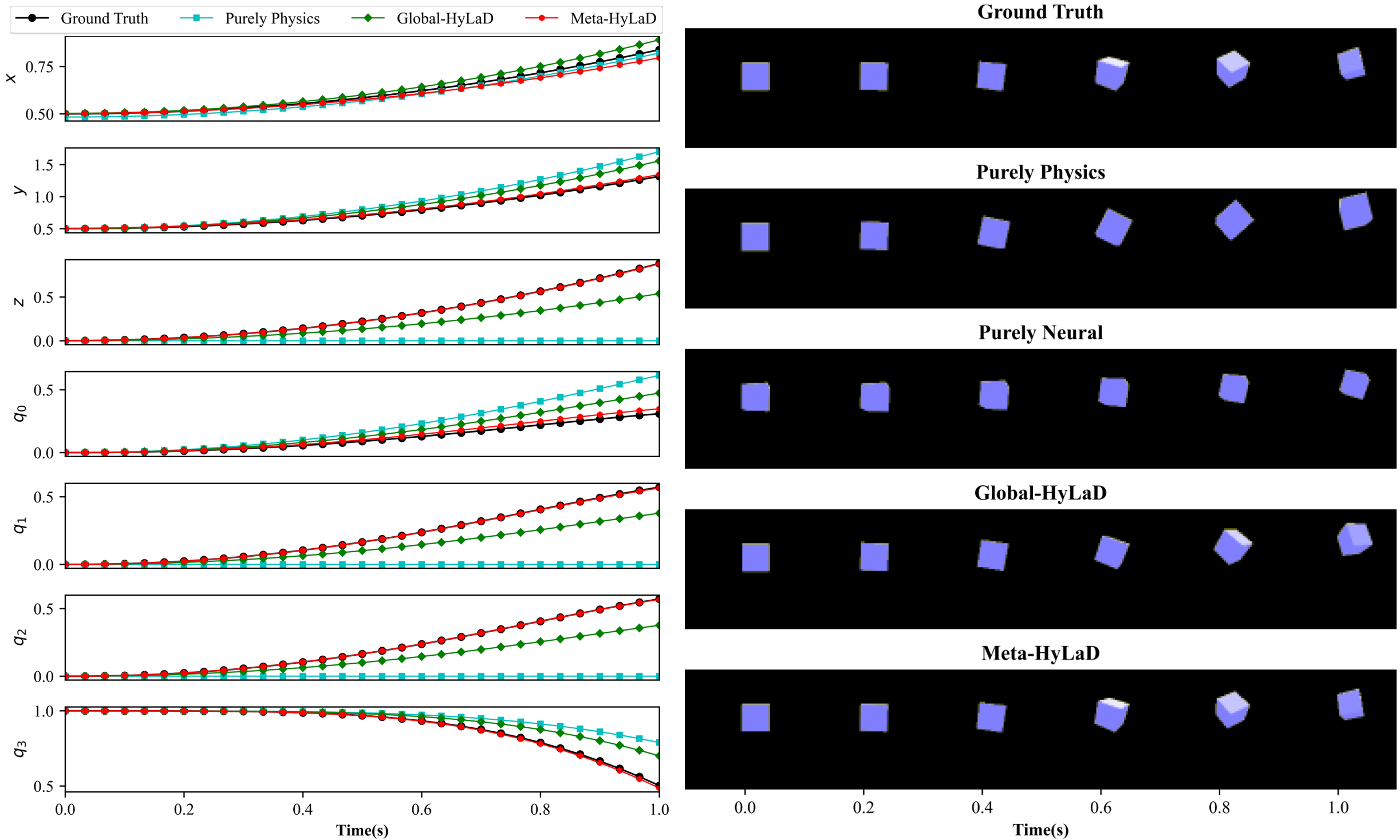
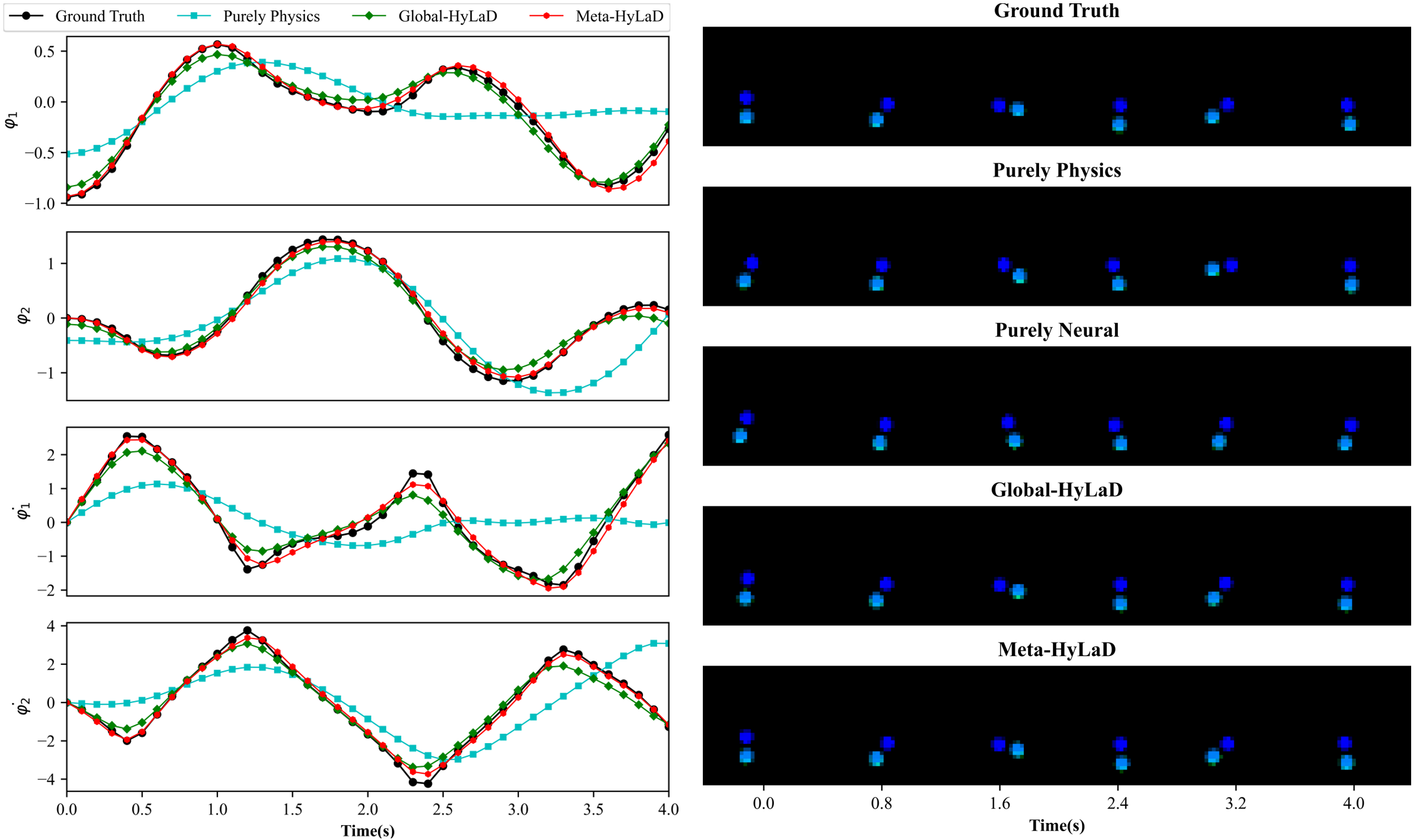
Models: We now fix the learn-to-identify strategy to that of Fig. 2B, and compare four alternatives of latent dynamic functions: using only the partial physics function (purely physics), using only a neural network (purely neural), hybrid as defined in Equation (2) but with a global (Global-HyLaD), and Meta-HyLaD. We also obtain results on a latent dynamic function utilizing the full physics, setting a performance reference when prior knowledge is perfect.
Metrics: We consider MSE for both the observed images and state variables , and Valid Prediction Time (VPT) that measures how long the predicted object’s trajectory remains close to the ground truth trajectory based on the MSE [2]. We separately evaluate these metrics for test time-series with parameters within (in distribution / ID) or outside (out of distribution / OOD) those used in the training data, as summarized in Table 1.
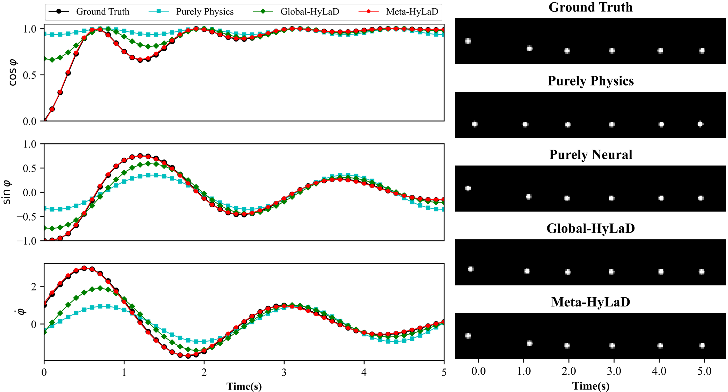
Results: Fig. 3 summarizes the results on three datasets, with complete results and visual examples provided in appendix C: note that the purely neural dynamic functions (yellow), due to the abstract nature of its latent state variables, results in poor MSE/VPT metrics on at a a magnitude larger than alternative approaches; their values are thus omitted from Fig. 3 but can be found in appendix C. As shown, purely physics-based approaches, when given perfect knowledge, achieve excellent performance as a reference (dashed blue line). Their accuracy, however, deteriorates substantially given imperfect knowledge (aqua), often to a level on par with purely neural approaches (yellow). The use of hybrid functions helps, although to a limited extent if the neural components are globally optimized (green). Meta-HyLaD (red), with an ability to identify the neural components from data, substantially improves over all three alternatives – its performance is on par with, and sometimes better than, the performance achieved with perfect physics.
4.4 Comparison with Existing Baselines
On the five physics systems, we then compare Meta-HyLaD with existing unsupervised latent dynamic models. Note that there is no existing hybrid latent dynamic models.
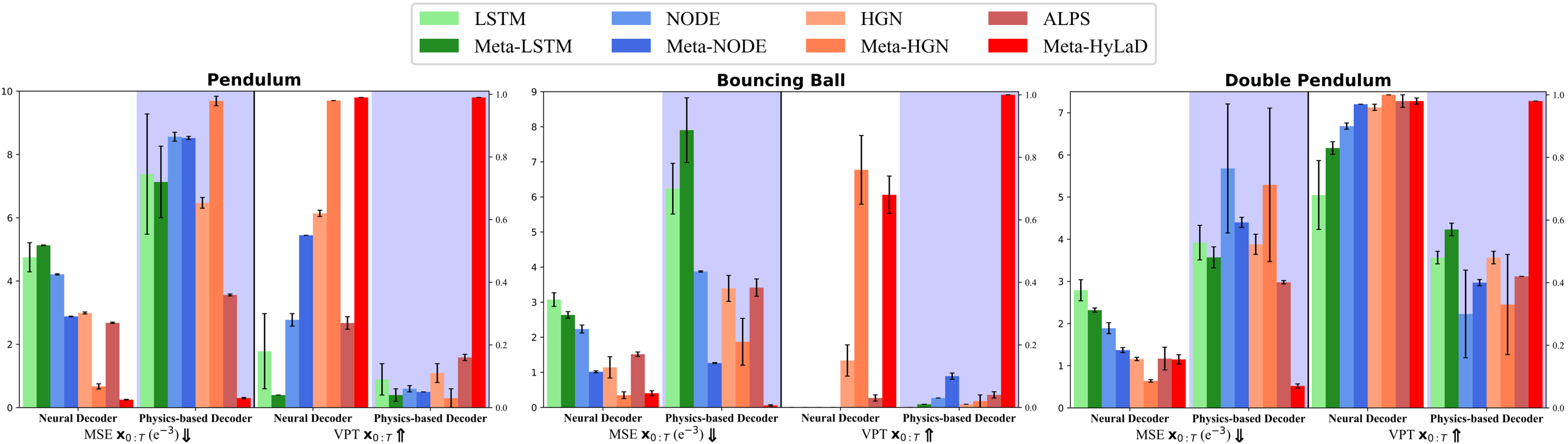
Models: We consider 1) ALPS [35] which considers a physics-based latent dynamic function (here the partial physics) and a reconstruction-based learning objective, and 2) three neural latent dynamic models ranging from those with minimal physics prior (LSTM and neural ODE / NODE) and strong prior (Hamiltonian generative network / HGN) [2]. We consider their original formulations [2] that optimize global latent dynamic functions as illustrated in Fig. 1B, as well as their extension to the presented meta-learning framework representative of recent works in meta-learning latent dynamics [18, 21]. Architecture details of all baselines are provided in appendix G. This provides a comprehensive coverage of prior arts in their choices of latent dynamic functions and identifications strateiges.
We further note that different decoders were used in these original baselines: the neural latent dynamic models utilize a neural network as the decoder (neural decoder) [2]; the latent-HGN utilizes a neural decoder but specifically uses the position latent state as the input (neural decoder with prior) [2]; ALPS uses both this and a physics-based decoder [35]. To isolate the effect of decoders, we further evaluate each of these baselines using each of the three different decoders.
Metrics: We consider MSE and VPT for , and omit metrics on due to its abstract nature in most baselines.
Results: Fig. 4 summarizes the results on three datasets for physics-based vs. neural decoders, with the complete quantitative results in appendix D. Notably, across all datasets, Meta-HyLaD in general demonstrates a significant margin of improvements over all baselines including those utilizing meta-learning. This improvement is the most significant when used in combination of a physics-based decoder while, with a neural decoder with or without prior, Meta-HyLaD sometimes becomes comparable with the meta-extension of HGN – this again demonstrates the benefits of physics inductive bias in both models. Note that, as we will show in Section 4.5, Meta-HyLaD is more generally applicable beyond Hamiltonian systems for which HGN is designed.
Interestingly, Meta-HyLaD improves with using a physics-based decoder, while the other baselines deteriorates. The effect of using a prior with the decoder (appendix C) is less consistent and varies with the dataset for all models.
4.5 Feasibility on Biomedical Systems: Dynamic PET
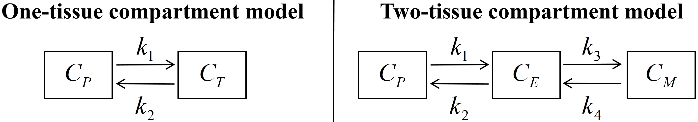
Finally, we consider recovering the spatial distribution and kinetics of radiotracer-labeled biological substrates from dynamic PET images. The regional tracker kinetics underlying PET can be described by the widely used compartment models in Table 1. The total concentration of radioactivity in all tissues, , on the scanning time interval is measured as: at each voxel . The activity image is obtained by lexicographic ordering of at different voxels. While raw PET data are sinograms, in this proof-of-concept we consider as the observed image series, with the goal to identify the compartment models. More details are in appendix E.
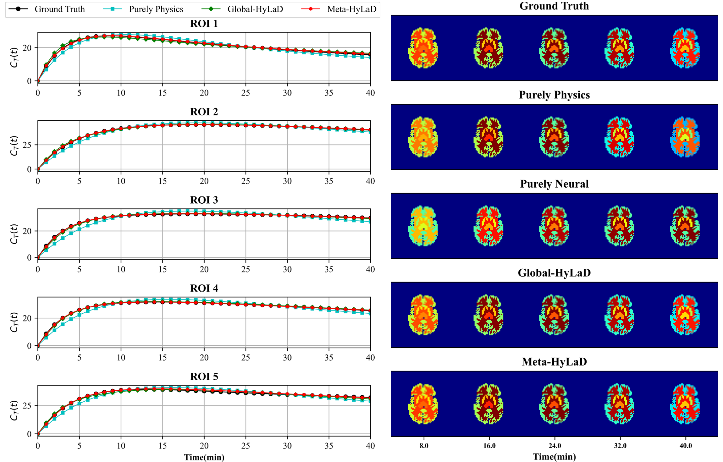
Data: We use the two-tissue compartment model listed in Table 1 to generate of a brain with 5 regions of interesting for 0-40 minutes with a scanning period of 0.5 minutes, resulting in 80 frames per time series. 2000 time-series samples are generated with training/test and ID/OOD split of parameter ranges provided in appendix E.
We then assume the one-tissue compartment model to be our prior physics in Meta-HyLaD. Compared to the additive and multiplicative errors considered earlier, this setup provides a more challenging scenario where the prior physics represents a crude approximation, i.e., , for the data-generating latent dynamics.
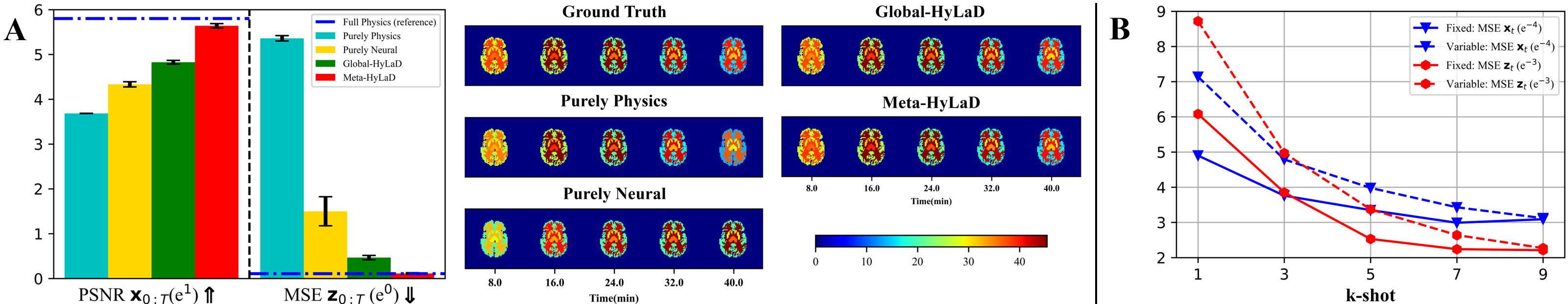
Model & Metrics: We compare Meta-HyLaD with purely physics, purely neural, and Global-HyLaD similar to Section 4.3. We consider MSE and peak signal-to-noise-ratio (PSNR) on , and MSE and VPT on , i.e., .
Results: Fig. 5A summarize the quantitative metrics along with visual examples, with the full results and examples of tracer kinetics in appendix E . The same observations in the physics systems still hold: Meta-HyLaD is the only model that is able to approach the reference performance (where data-generating physics is used in the identification), significantly outperforming the alternatives. This leaves exciting future real-world opportunities for Meta-HyLaD.
5 Conclusions & Discussion
We present Meta-HyLaD as a first solution to unsupervised learning of hybrid latent dynamics, demonstrating the use of physics inductive bias combined with the learning-to-identify strategy to effectively leverage prior knowledge while identifying its unknown gap to observed data.
The effect of the size of context set: Fig. 5B shows that, while increasing the context-set size increases the performance of Meta-HyLaD, at it still significantly outperforms the various baselines. It is also minimally affected when trained with variable size of , enhancing its ability to accommodate varying availability of context samples at test time. If there is no knowledge about which samples share the same dynamics, future solutions may be to replace the averaging function in context-set embedding with attention mechanisms, to learn to extract similar context samples. Additional ablation results are provided in appendix F.
Generality and failure modes: In section F.3, we provide examples that Meta-HyLaD can accommodate general design choices of and maintains its strong identification and forecasting performance. We also probe the potential failure modes for Meta-HyLaD and its use of decoders. As shown in section F.4, if representing prior physics becomes too weak, e.g., modeling only the dampening effect on Pendulum, Meta-HyLaD may degenerate to a performance similar to purely neural approaches for forecasting , although still with a substantial gain in the accuracy of . Finally, while neural decoders provide competitive performance for all models considered, they could fail if the data-generating decoder function is not global. In this setting, we show that the same learn-to-identify strategy can be extended to adapt the decoder (section F.5), leaving another future avenue of Meta-HyLaD to be pursued.
Acknowledgements
This work is supported in part by the National Key Research and Development Program of China(No: 2020AAA0109502); the Talent Program of Zhejiang Province (No: 2021R51004); NIH NHLBI grant R01HL145590 and NSF OAC-2212548. This paper presents work whose goal is to advance the field of Machine Learning. There are many potential societal consequences of our work, none which we feel must be specifically highlighted here.
References
- [1] Allen-Blanchette, C., Veer, S., Majumdar, A., Leonard, N.E.: Lagnetvip: A lagrangian neural network for video prediction. arXiv preprint arXiv:2010.12932 (2020)
- [2] Botev, A., Jaegle, A., Wirnsberger, P., Hennes, D., Higgins, I.: Which priors matter? benchmarking models for learning latent dynamics (2021)
- [3] Choudhary, A., Lindner, J.F., Holliday, E.G., Miller, S.T., Sinha, S., Ditto, W.L.: Forecasting hamiltonian dynamics without canonical coordinates. Nonlinear Dynamics 103, 1553–1562 (2021)
- [4] Chung, J., Kastner, K., Dinh, L., Goel, K., Courville, A.C., Bengio, Y.: A recurrent latent variable model for sequential data. Advances in neural information processing systems 28 (2015)
- [5] Chung, J., Kastner, K., Dinh, L., Goel, K., Courville, A.C., Bengio, Y.: A recurrent latent variable model for sequential data. Advances in neural information processing systems 28 (2015)
- [6] Cranmer, M., Greydanus, S., Hoyer, S., Battaglia, P., Spergel, D., Ho, S.: Lagrangian neural networks. In: ICLR 2020 Workshop on Integration of Deep Neural Models and Differential Equations (2020)
- [7] Feng, D., Huang, S.C., Wang, X.: Models for computer simulation studies of input functions for tracer kinetic modeling with positron emission tomography. International journal of bio-medical computing 32(2), 95–110 (1993)
- [8] Fraccaro, M., Kamronn, S., Paquet, U., Winther, O.: A disentangled recognition and nonlinear dynamics model for unsupervised learning. Advances in neural information processing systems 30 (2017)
- [9] Girin, L., Leglaive, S., Bie, X., Diard, J., Hueber, T., Alameda-Pineda, X.: Dynamical variational autoencoders: A comprehensive review. Foundations and Trends in Machine Learning 15(1-2), 1–175 (2021)
- [10] Golemo, F., Taiga, A.A., Courville, A., Oudeyer, P.Y.: Sim-to-real transfer with neural-augmented robot simulation. In: Conference on Robot Learning. pp. 817–828. PMLR (2018)
- [11] Greydanus, S., Dzamba, M., Yosinski, J.: Hamiltonian neural networks. Advances in neural information processing systems 32 (2019)
- [12] Gupta, J.K., Menda, K., Manchester, Z., Kochenderfer, M.J.: A general framework for structured learning of mechanical systems. arXiv preprint arXiv:1902.08705 (2019)
- [13] Heiden, E., Millard, D., Coumans, E., Sheng, Y., Sukhatme, G.S.: Neuralsim: Augmenting differentiable simulators with neural networks. In: 2021 IEEE International Conference on Robotics and Automation (ICRA). pp. 9474–9481. IEEE (2021)
- [14] Higgins, I., Wirnsberger, P., Jaegle, A., Botev, A.: Symetric: Measuring the quality of learnt hamiltonian dynamics inferred from vision. Advances in Neural Information Processing Systems 34, 25591–25605 (2021)
- [15] Hong, J., Brendel, M., Erlandsson, K., Sari, H., Lu, J., Clement, C., Bui, N.V., Meindl, M., Ziegler, S., Barthel, H., et al.: Forecasting the pharmacokinetics with limited early frames in dynamic brain pet imaging using neural ordinary differential equation. IEEE Transactions on Radiation and Plasma Medical Sciences (2023)
- [16] Hwangbo, J., Lee, J., Dosovitskiy, A., Bellicoso, D., Tsounis, V., Koltun, V., Hutter, M.: Learning agile and dynamic motor skills for legged robots. Science Robotics 4(26), eaau5872 (2019)
- [17] Jaques, M., Burke, M., Hospedales, T.: Physics-as-inverse-graphics: Unsupervised physical parameter estimation from video. In: Eighth International Conference on Learning Representations. pp. 1–16 (2020)
- [18] Jiang, X., Missel, R., Li, Z., Wang, L.: Sequential latent variable models for few-shot high-dimensional time-series forecasting. In: The Eleventh International Conference on Learning Representations (2022)
- [19] Karl, M., Soelch, M., Bayer, J., Van der Smagt, P.: Deep variational bayes filters: Unsupervised learning of state space models from raw data. arXiv preprint arXiv:1605.06432 (2016)
- [20] Karl, M., Soelch, M., Bayer, J., van der Smagt, P.: Deep variational bayes filters: Unsupervised learning of state space models from raw data. In: International Conference on Learning Representations (2016)
- [21] Kirchmeyer, M., Yin, Y., Donà, J., Baskiotis, N., Rakotomamonjy, A., Gallinari, P.: Generalizing to new physical systems via context-informed dynamics model. In: International Conference on Machine Learning. pp. 11283–11301. PMLR (2022)
- [22] Klushyn, A., Kurle, R., Soelch, M., Cseke, B., van der Smagt, P.: Latent matters: Learning deep state-space models. Advances in Neural Information Processing Systems 34, 10234–10245 (2021)
- [23] Krishnan, R., Shalit, U., Sontag, D.: Structured inference networks for nonlinear state space models. In: Proceedings of the AAAI Conference on Artificial Intelligence. vol. 31 (2017)
- [24] Lutter, M., Ritter, C., Peters, J.: Deep lagrangian networks: Using physics as model prior for deep learning. In: International Conference on Learning Representations (ICLR 2019). OpenReview. net (2019)
- [25] Murthy, J.K., Macklin, M., Golemo, F., Voleti, V., Petrini, L., Weiss, M., Considine, B., Parent-Lévesque, J., Xie, K., Erleben, K., et al.: gradsim: Differentiable simulation for system identification and visuomotor control. In: International conference on learning representations (2020)
- [26] Oreshkin, B.N., Carpov, D., Chapados, N., Bengio, Y.: Meta-learning framework with applications to zero-shot time-series forecasting. In: Proceedings of the AAAI Conference on Artificial Intelligence. vol. 35, pp. 9242–9250 (2021)
- [27] Phelps, M.E.: Molecular imaging and its biological applications. Eur J Nucl Med Mol Imaging 31, 1544 (2004)
- [28] Queiruga, A., Erichson, N.B., Hodgkinson, L., Mahoney, M.W.: Stateful ode-nets using basis function expansions. Advances in Neural Information Processing Systems 34, 21770–21781 (2021)
- [29] Rackauckas, C., Ma, Y., Martensen, J., Warner, C., Zubov, K., Supekar, R., Skinner, D., Ramadhan, A., Edelman, A.: Universal differential equations for scientific machine learning. arXiv preprint arXiv:2001.04385 (2020)
- [30] Saemundsson, S., Terenin, A., Hofmann, K., Deisenroth, M.: Variational integrator networks for physically structured embeddings. In: International Conference on Artificial Intelligence and Statistics. pp. 3078–3087. PMLR (2020)
- [31] Sung, F., Yang, Y., Zhang, L., Xiang, T., Torr, P.H., Hospedales, T.M.: Learning to compare: Relation network for few-shot learning. In: Proceedings of the IEEE conference on computer vision and pattern recognition. pp. 1199–1208 (2018)
- [32] Toth, P., Rezende, D.J., Jaegle, A., Racanière, S., Botev, A., Higgins, I.: Hamiltonian generative networks. arXiv preprint arXiv:1909.13789 (2019)
- [33] Wang, R., Walters, R., Yu, R.: Meta-learning dynamics forecasting using task inference. Advances in Neural Information Processing Systems 35, 21640–21653 (2022)
- [34] Wang, R., Walters, R., Yu, R.: Meta-learning dynamics forecasting using task inference. Advances in Neural Information Processing Systems 35, 21640–21653 (2022)
- [35] Yang, T.Y., Rosca, J., Narasimhan, K., Ramadge, P.J.: Learning physics constrained dynamics using autoencoders. Advances in Neural Information Processing Systems 35, 17157–17172 (2022)
- [36] Yildiz, C., Heinonen, M., Lahdesmaki, H.: Ode2vae: Deep generative second order odes with bayesian neural networks. Advances in Neural Information Processing Systems 32 (2019)
- [37] Yin, Y., Ayed, I., de Bézenac, E., Baskiotis, N., Gallinari, P.: Leads: Learning dynamical systems that generalize across environments. Advances in Neural Information Processing Systems 34, 7561–7573 (2021)
- [38] Zeng, A., Song, S., Lee, J., Rodriguez, A., Funkhouser, T.: Tossingbot: Learning to throw arbitrary objects with residual physics. IEEE Transactions on Robotics 36(4), 1307–1319 (2020)
- [39] Zhong, Y.D., Dey, B., Chakraborty, A.: Symplectic ode-net: Learning hamiltonian dynamics with control. In: International Conference on Learning Representations (2019)
- [40] Zhong, Y.D., Leonard, N.: Unsupervised learning of lagrangian dynamics from images for prediction and control. Advances in Neural Information Processing Systems 33, 10741–10752 (2020)
Appendix A Data Details and Experimental Settings of Physics Systems
Here we provide complete data details and experimental settings of physics systems and the overview of physics systems can be seen in Fig. 6. The ratio of training samples:ID testing samples:OOD testing samples is roughly 6:2:2 in all datasets.
A.1 Data Details
(1) Pendulum: The dynamic equation is: , where is the angle, is the angular velocity, are the gravitational constant and the damping coefficient, and is the length of the pendulum. We fix , then sample , , , ID: and OOD: . We generate a 25 step in time domain [0.0s, 5.0s] following the dynamic equation, and render corresponding 32 by 32 by 1 pixel observation snapshots. In total, we generate 15390 training and test sequences.
(2) Mass Spring: The dynamic equation is: , where , , are the positions of node1 and node2, are the velocities of node1 and node2 and are the stiffness and damping coefficient of the spring and damper. We fix , then sample , ID: and OOD: . We generate a 25 step in time domain [0.0s, 5.0s] following the dynamic equation, and render corresponding 32 by 32 by 3 pixel observation snapshots. In total, we generate 12960 training and test sequences.
(3) Bouncing Ball: The dynamic equation is: , where are the amplitude and direction of gravity. When there is a collision, or . We set the collision position at . We fix , then sample , , ID: and OOD: . We generate a 25 step in time domain [0.0s, 2.5s] following the dynamic equation, and render corresponding 32 by 32 by 1 pixel observation snapshots. In total, we generate 21060 training and test sequences.
(4) Rigid Body: We represent the state of a 3D cube as consisting of a position and a quaternion . The generalized velocity of the cube is and its dynamic equation is: , where are the mass and inertia matrix, and are the magnitude of the force, its direction in the xy-plane and its direction with respect to the z-axis. We fix and , then sample , ID: and OOD: . We generate a 30 step in time domain [0.0s, 1.0s] following the dynamic equation, and render corresponding 64 by 64 by 3 pixel observation snapshots. In total, we generate 4800 training and test sequences.
(5) Double Pendulum: The dynamic equation is: , where ,
, and are the mass of two pendulums. We fix , then sample , ID: and OOD: . We generate a 40 step in time domain [0.0s, 4.0s] following the dynamic equation, and render corresponding 32 by 32 by 3 pixel observation snapshots. In total, we generate 12705 training and test sequences.
A.2 Experimental Settings for section 4.3
Here we provide specific forms of different latent dynamic functions in section 4.3 for each datasets.
A.2.1 Pendulum
| Dynamics | Equation |
|---|---|
| Full Physics | |
| Purely Physics | |
| Purely Neural | |
| Global-HyLaD | |
| Meta-HyLaD |
A.2.2 Mass Spring
| Dynamics | Equation |
|---|---|
| Full Physics | |
| Purely Physics | |
| Purely Neural | |
| Global-HyLaD | |
| Meta-HyLaD |
A.2.3 Bouncing Ball
| Dynamics | Equation |
|---|---|
| Full Physics | |
| Purely Physics | |
| Purely Neural | |
| Global-HyLaD | |
| Meta-HyLaD |
A.2.4 Rigid Body
| Dynamics | Equation |
|---|---|
| Full Physics | |
| Purely Physics | |
| Purely Neural | |
| Global-HyLaD | |
| Meta-HyLaD |
A.2.5 Double Pendulum
| Dynamics | Equation |
|---|---|
| Full Physics | |
| Purely Physics | |
| Purely Neural | |
| Global-HyLaD | |
| Meta-HyLaD |
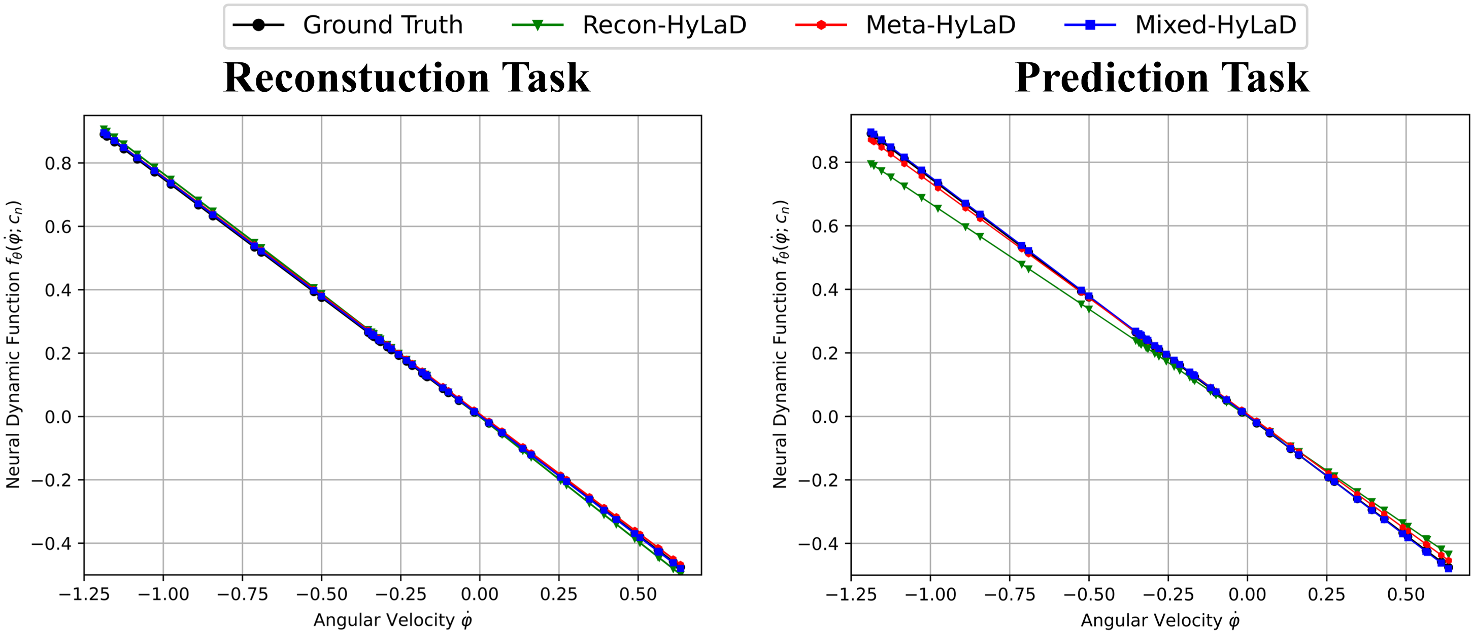
Appendix B Examples of Identified Neural Dynamic Functions (Additioanl Results for section 4.2)
We also visualize the neural dynamic function of three learning strategies and ground truth , see Fig 7. From figure, we can clearly see that all three learning strategies perform well on reconstruction task, but Recon-HyLaD will fail on prediction task, which shows that a good reconstruction is not sufficient evidence that the underlying latent dynamics is correctly identified and the learn-to-identify strategy is an effective solution to address this issue of identifiability.
Appendix C Additional Results of section 4.3: Benefits of Hybrid Dynamics
Here we provide complete experimental results and some visual examples of section 4.3.
C.1 Pendulum
| Dynamics | Data | MSE (e-3) | MSE (e-2) | VPT | VPT of |
|---|---|---|---|---|---|
| Full Physics (oracle) | ID | 0.31(0.05) | 0.24(0.06) | 0.99(0.00) | 0.98(0.01) |
| OOD | 0.62(0.06) | 0.48(0.08) | 0.97(0.01) | 0.88(0.03) | |
| Purely Physics | ID | 4.38(0.00) | 13.09(0.18) | 0.13(0.19) | 0.05(0.01) |
| OOD | 4.94(0.07) | 19.57(0.55) | 0.05(0.00) | 0.01(0.00) | |
| Purely Neural | ID | 3.36(0.52) | 109.96(54.82) | 0.53(0.07) | 0.00(0.00) |
| OOD | 4.02(0.54) | 78.47(35.18) | 0.43(0.03) | 0.00(0.00) | |
| Global-HyLaD | ID | 2.26(0.05) | 4.01(0.05) | 0.60(0.01) | 0.41(0.01) |
| OOD | 2.99(0.06) | 6.50(0.02) | 0.38(0.02) | 0.17(0.00) | |
| Meta-HyLaD | ID | 0.30(0.01) | 0.22(0.00) | 0.99(0.00) | 0.98(0.00) |
| OOD | 0.25(0.02) | 0.17(0.02) | 0.99(0.00) | 0.95(0.01) |
C.2 Mass Spring
| Dynamics | Data | MSE (e-4) | MSE (e-2) | VPT | VPT of |
|---|---|---|---|---|---|
| Full Physics (oracle) | ID | 0.12(0.01) | 0.09(0.02) | 1.00(0.00) | 1.00(0.00) |
| OOD | 0.40(0.03) | 0.46(0.07) | 0.98(0.01) | 0.88(0.02) | |
| Purely Physics | ID | 6.32(0.09) | 19.01(0.56) | 0.44(0.09) | 0.14(0.00) |
| OOD | 8.83(0.03) | 27.93(0.21) | 0.17(0.00) | 0.05(0.00) | |
| Purely Neural | ID | 1.86(0.13) | 393.47(75.06) | 0.91(0.01) | 0.05(0.00) |
| OOD | 2.51(0.39) | 348.02(93.33) | 0.77(0.07) | 0.05(0.00) | |
| Global-HyLaD | ID | 1.53(0.01) | 3.20(0.13) | 0.92(0.01) | 0.70(0.03) |
| OOD | 2.45(0.05) | 4.68(0.16) | 0.76(0.02) | 0.28(0.02) | |
| Meta-HyLaD | ID | 0.13(0.03) | 0.09(0.02) | 1.00(0.00) | 1.00(0.00) |
| OOD | 0.19(0.07) | 0.12(0.06) | 1.00(0.00) | 0.98(0.01) |
C.3 Bouncing Ball
| Dynamics | Data | MSE (e-2) | MSE (e-1) | VPT | VPT of |
|---|---|---|---|---|---|
| Full Physics (oracle) | ID | 0.05(0.02) | 0.03(0.02) | 1.00(0.01) | 0.96(0.04) |
| OOD | 0.14(0.06) | 0.14(0.09) | 0.93(0.04) | 0.84(0.06) | |
| Purely Physics | ID | 3.20(0.10) | 15.54(0.16) | 0.09(0.02) | 0.04(0.02) |
| OOD | 3.67(0.13) | 17.73(0.70) | 0.03(0.01) | 0.01(0.00) | |
| Purely Neural | ID | 1.26(0.01) | 2.55(0.01) | 0.10(0.01) | 0.02(0.00) |
| OOD | 1.92(0.23) | 7.26(2.98) | 0.12(0.02) | 0.03(0.01) | |
| Global-HyLaD | ID | 2.15(0.04) | 8.33(0.19) | 0.21(0.03) | 0.12(0.02) |
| OOD | 3.24(0.04) | 15.21(0.32) | 0.06(0.00) | 0.03(0.00) | |
| Meta-HyLaD | ID | 0.06(0.02) | 0.03(0.01) | 1.00(0.00) | 0.94(0.03) |
| OOD | 0.16(0.05) | 0.17(0.07) | 0.92(0.02) | 0.80(0.05) |
C.4 Rigid Body
| Dynamics | Data | MSE (e-3) | MSE (e-2) | VPT | VPT of |
|---|---|---|---|---|---|
| Full Physics (oracle) | ID | 0.37(0.19) | 0.02(0.01) | 1.00(0.01) | 1.00(0.00) |
| OOD | 1.26(0.02) | 0.09(0.00) | 0.94(0.03) | 0.98(0.02) | |
| Purely Physics | ID | 6.46(0.08) | 2.56(0.02) | 0.59(0.00) | 0.59(0.00) |
| OOD | 18.23(0.23) | 10.36(0.24) | 0.29(0.00) | 0.38(0.00) | |
| Purely Neural | ID | 5.01(0.17) | 15.92(0.93) | 0.58(0.01) | 0.00(0.00) |
| OOD | 12.29(0.27) | 19.56(0.39) | 0.36(0.03) | 0.00(0.00) | |
| Global-HyLaD | ID | 2.90(0.33) | 0.48(0.08) | 0.79(0.02) | 0.86(0.01) |
| OOD | 14.41(0.92) | 5.28(1.00) | 0.34(0.02) | 0.46(0.02) | |
| Meta-HyLaD | ID | 0.74(0.34) | 0.05(0.04) | 0.98(0.02) | 0.99(0.01) |
| OOD | 1.74(0.12) | 0.13(0.01) | 0.90(0.01) | 0.97(0.00) |
C.5 Double Pendulum
| Dynamics | Data | MSE (e-3) | MSE (e-1) | VPT | VPT of |
|---|---|---|---|---|---|
| Full Physics (oracle) | ID | 0.18(0.01) | 0.13(0.01) | 1.00(0.00) | 0.99(0.00) |
| OOD | 0.92(0.11) | 2.14(0.37) | 0.95(0.01) | 0.95(0.00) | |
| Purely Physics | ID | 3.93(0.01) | 8.37(0.89) | 0.47(0.01) | 0.36(0.01) |
| OOD | 3.03(0.08) | 4.08(0.51) | 0.56(0.03) | 0.59(0.02) | |
| Purely Neural | ID | 3.41(0.02) | 35.73(0.00) | 0.61(0.00) | 0.13(0.01) |
| OOD | 4.10(0.17) | 37.35(0.00) | 0.57(0.04) | 0.14(0.01) | |
| Global-HyLaD | ID | 1.64(0.01) | 2.79(0.03) | 0.86(0.00) | 0.78(0.00) |
| OOD | 2.84(0.17) | 6.55(0.26) | 0.72(0.03) | 0.75(0.01) | |
| Meta-HyLaD | ID | 0.52(0.05) | 0.38(0.03) | 0.98(0.00) | 0.93(0.00) |
| OOD | 1.10(0.06) | 2.97(0.19) | 0.94(0.01) | 0.95(0.01) |
Appendix D Complete Results of section 4.4: Comparison with Baselines
Here we provide complete experimental results of section 4.4.
| Pendulum | |||||||
|---|---|---|---|---|---|---|---|
| Physics-based Decoder | Neural Decoder with prior | Neural Decoder no prior | |||||
| Model | Data | MSE(e-3) | VPT | MSE(e-3) | VPT | MSE(e-3) | VPT |
| LSTM | ID | 7.38(1.90) | 0.09(0.05) | / | / | 4.75(0.46) | 0.18(0.12) |
| OOD | 5.36(0.74) | 0.10(0.03) | / | / | 4.09(0.19) | 0.19(0.12) | |
| Meta-LSTM | ID | 7.13(1.13) | 0.04(0.02) | / | / | 5.13(0.01) | 0.04(0.00) |
| OOD | 5.16(0.49) | 0.04(0.01) | / | / | 3.68(0.01) | 0.04(0.00) | |
| NODE | ID | 8.56(0.14) | 0.06(0.01) | / | / | 4.21(0.02) | 0.28(0.02) |
| OOD | 5.16(0.44) | 0.07(0.01) | / | / | 3.85(0.11) | 0.30(0.03) | |
| Meta-NODE | ID | 8.52(0.05) | 0.05(0.00) | / | / | 2.88(0.01) | 0.55(0.00) |
| OOD | 5.35(0.11) | 0.07(0.00) | / | / | 3.50(0.10) | 0.43(0.01) | |
| HGN | ID | 6.47(0.17) | 0.11(0.03) | 3.53(0.02) | 0.48(0.01) | 2.99(0.03) | 0.62(0.01) |
| OOD | 5.64(0.27) | 0.09(0.03) | 3.69(0.15) | 0.37(0.02) | 3.10(0.17) | 0.47(0.03) | |
| Meta-HGN | ID | 9.69(0.15) | 0.03(0.00) | 3.04(0.17) | 0.54(0.01) | 0.67(0.08) | 0.98(0.00) |
| OOD | 6.24(0.14) | 0.04(0.00) | 3.69(0.08) | 0.42(0.01) | 0.72(0.05) | 0.91(0.02) | |
| ALPS | ID | 3.56(0.03) | 0.16(0.01) | 2.70(0.01) | 0.28(0.01) | 2.68(0.02) | 0.27(0.02) |
| OOD | 4.17(0.00) | 0.04(0.00) | 3.28(0.01) | 0.06(0.00) | 3.25(0.03) | 0.06(0.00) | |
| Meta-HyLaD | ID | 0.30(0.02) | 0.99(0.00) | 0.29(0.03) | 0.99(0.00) | 0.25(0.01) | 0.99(0.00) |
| OOD | 0.31(0.06) | 0.99(0.00) | 0.25(0.02) | 0.99(0.00) | 0.20(0.04) | 1.00(0.00) | |
| Mass Spring | |||||||
| Physics-based Decoder | Neural Decoder with prior | Neural Decoder no prior | |||||
| Model | Data | MSE(e-3) | VPT | MSE(e-3) | VPT | MSE(e-3) | VPT |
| LSTM | ID | 16.59(12.95) | 0.01(0.01) | / | / | 0.40(0.03) | 0.56(0.06) |
| OOD | 16.51(13.11) | 0.01(0.01) | / | / | 0.20(0.02) | 0.67(0.09) | |
| Meta-LSTM | ID | 19.48(8.84) | 0.00(0.00) | / | / | 0.40(0.03) | 0.59(0.06) |
| OOD | 19.44(8.94) | 0.00(0.00) | / | / | 0.20(0.01) | 0.60(0.02) | |
| NODE | ID | 0.80(0.01) | 0.15(0.01) | / | / | 0.38(0.01) | 0.62(0.02) |
| OOD | 0.38(0.01) | 0.25(0.01) | / | / | 0.19(0.01) | 0.67(0.03) | |
| Meta-NODE | ID | 0.69(0.09) | 0.21(0.05) | / | / | 0.27(0.02) | 0.77(0.01) |
| OOD | 0.26(0.10) | 0.44(0.16) | / | / | 0.24(0.01) | 0.69(0.02) | |
| HGN | ID | 10.33(7.47) | 0.00(0.00) | 0.27(0.02) | 0.84(0.02) | 0.15(0.01) | 0.95(0.01) |
| OOD | 10.11(7.60) | 0.23(0.03) | 0.11(0.01) | 0.78(0.04) | 0.11(0.01) | 0.85(0.03) | |
| Meta-HGN | ID | 5.96(3.90) | 0.00(0.00) | 0.18(0.02) | 0.85(0.03) | 0.08(0.02) | 1.00(0.00) |
| OOD | 5.66(3.96) | 0.00(0.00) | 0.18(0.03) | 0.76(0.02) | 0.06(0.01) | 0.99(0.00) | |
| ALPS | ID | 17.52(7.60) | 0.00(0.00) | 2.59(0.80) | 0.03(0.03) | 1.40(0.59) | 0.10(0.10) |
| OOD | 17.67(7.64) | 0.00(0.00) | 2.25(1.07) | 0.05(0.05) | 1.16(0.61) | 0.13(0.11) | |
| Meta-HyLaD | ID | 0.01(0.00) | 1.00(0.00) | 0.03(0.00) | 1.00(0.00) | 0.04(0.01) | 1.00(0.00) |
| OOD | 0.02(0.01) | 1.00(0.00) | 0.03(0.00) | 1.00(0.00) | 0.03(0.01) | 1.00(0.00) | |
| Bouncing Ball | |||||||
|---|---|---|---|---|---|---|---|
| Physics-based Decoder | Neural Decoder with prior | Neural Decoder no prior | |||||
| Model | Data | MSE(e-3) | VPT | MSE(e-3) | VPT | MSE(e-3) | VPT |
| LSTM | ID | 62.35(7.22) | 0.00(0.00) | / | / | 30.74(1.94) | 0.00(0.00) |
| OOD | 60.29(5.78) | 0.00(0.00) | / | / | 34.25(0.29) | 0.00(0.00) | |
| Meta-LSTM | ID | 79.03(9.22) | 0.01(0.00) | / | / | 26.37(0.93) | 0.00(0.00) |
| OOD | 76.66(11.14) | 0.01(0.00) | / | / | 35.84(2.29) | 0.00(0.00) | |
| NODE | ID | 38.74(0.17) | 0.03(0.00) | / | / | 22.33(1.13) | 0.00(0.00) |
| OOD | 42.17(0.73) | 0.01(0.00) | / | / | 33.37(1.18) | 0.00(0.00) | |
| Meta-NODE | ID | 12.64(0.14) | 0.10(0.01) | / | / | 10.16(0.28) | 0.00(0.00) |
| OOD | 19.21(2.33) | 0.12(0.02) | / | / | 18.04(7.94) | 0.10(0.00) | |
| HGN | ID | 33.92(3.69) | 0.01(0.00) | 15.65(7.04) | 0.06(0.02) | 11.41(3.04) | 0.15(0.05) |
| OOD | 39.46(5.69) | 0.01(0.01) | 18.88(4.98) | 0.07(0.01) | 21.40(1.72) | 0.07(0.02) | |
| Meta-HGN | ID | 18.70(6.67) | 0.02(0.01) | 3.87(0.27) | 0.70(0.04) | 3.48(0.97) | 0.76(0.11) |
| OOD | 25.85(4.39) | 0.01(0.01) | 14.69(7.79) | 0.50(0.13) | 32.09(6.54) | 0.31(0.04) | |
| ALPS | ID | 34.15(2.46) | 0.04(0.01) | 21.40(0.20) | 0.03(0.00) | 15.15(0.63) | 0.03(0.01) |
| OOD | 33.95(1.22) | 0.01(0.00) | 24.92(1.12) | 0.02(0.01) | 23.54(4.06) | 0.02(0.01) | |
| Meta-HyLaD | ID | 0.56(0.19) | 1.00(0.00) | 2.13(1.37) | 0.94(0.08) | 4.05(0.71) | 0.68(0.06) |
| OOD | 1.60(0.50) | 0.92(0.02) | 4.46(1.25) | 0.81(0.04) | 5.92(1.22) | 0.61(0.02) | |
| Rigid Body | |||||||
| Physics-based Decoder | Neural Decoder with prior | Neural Decoder no prior | |||||
| Model | Data | MSE(e-3) | VPT | MSE(e-3) | VPT | MSE(e-3) | VPT |
| LSTM | ID | 21.43(3.99) | 0.02(0.03) | / | / | 10.40(0.11) | 0.35(0.01) |
| OOD | 19.63(5.15) | 0.02(0.04) | / | / | 7.60(0.46) | 0.43(0.02) | |
| Meta-LSTM | ID | 18.80(4.85) | 0.06(0.05) | / | / | 3.97(0.69) | 0.72(0.11) |
| OOD | 16.66(6.27) | 0.08(0.07) | / | / | 5.58(1.77) | 0.60(0.15) | |
| NODE | ID | 17.73(6.42) | 0.22(0.18) | / | / | 9.29(0.01) | 0.42(0.00) |
| OOD | 15.55(8.24) | 0.27(0.23) | / | / | 6.33(0.07) | 0.50(0.00) | |
| Meta-NODE | ID | 4.65(1.56) | 0.60(0.11) | / | / | 1.51(0.08) | 0.99(0.00) |
| OOD | 5.00(1.98) | 0.58(0.15) | / | / | 1.70(0.10) | 0.96(0.02) | |
| HGN | ID | 11.76(3.42) | 0.32(0.01) | 2.65(0.13) | 0.85(0.02) | 6.36(0.66) | 0.61(0.02) |
| OOD | 10.38(1.61) | 0.35(0.08) | 3.87(0.47) | 0.73(0.04) | 11.59(1.97) | 0.47(0.02) | |
| Meta-HGN | ID | 6.77(1.56) | 0.61(0.02) | 1.44(0.04) | 1.00(0.00) | 5.45(0.22) | 0.62(0.03) |
| OOD | 7.30(2.10) | 0.98(0.02) | 1.62(0.03) | 0.98(0.01) | 5.53(1.03) | 0.62(0.08) | |
| ALPS | ID | 5.03(0.57) | 0.54(0.05) | 2.53(0.18) | 0.92(0.03) | 5.77(1.13) | 0.54(0.12) |
| OOD | 3.57(0.14) | 0.64(0.02) | 2.81(0.15) | 0.85(0.03) | 10.62(2.91) | 0.42(0.14) | |
| Meta-HyLaD | ID | 0.74(0.34) | 0.98(0.02) | 1.75(0.10) | 0.99(0.00) | 5.11(0.22) | 0.63(0.02) |
| OOD | 1.74(0.13) | 0.90(0.01) | 1.80(0.07) | 0.99(0.01) | 7.69(2.08) | 0.47(0.08) | |
| Double Pendulum | |||||||
| Physics-based Decoder | Neural Decoder with prior | Neural Decoder no prior | |||||
| Model | Data | MSE(e-3) | VPT | MSE(e-3) | VPT | MSE(e-3) | VPT |
| LSTM | ID | 3.92(0.41) | 0.48(0.02) | / | / | 2.79(0.25) | 0.68(0.11) |
| OOD | 4.64(0.28) | 0.43(0.01) | / | / | 3.05(0.25) | 0.60(0.08) | |
| Meta-LSTM | ID | 3.57(0.25) | 0.57(0.02) | / | / | 2.32(0.05) | 0.83(0.02) |
| OOD | 4.25(0.15) | 0.53(0.02) | / | / | 2.59(0.06) | 0.76(0.02) | |
| NODE | ID | 5.68(1.53) | 0.30(0.14) | / | / | 1.89(0.13) | 0.90(0.01) |
| OOD | 6.03(1.46) | 0.26(0.14) | / | / | 2.42(0.08) | 0.78(0.01) | |
| Meta-NODE | ID | 4.40(0.12) | 0.40(0.01) | / | / | 1.37(0.06) | 0.97(0.00) |
| OOD | 4.87(0.35) | 0.36(0.01) | / | / | 2.05(0.05) | 0.84(0.01) | |
| HGN | ID | 3.88(0.24) | 0.48(0.02) | 1.61(0.03) | 0.91(0.01) | 1.16(0.04) | 0.96(0.01) |
| OOD | 4.57(0.33) | 0.44(0.01) | 2.25(0.10) | 0.78(0.01) | 1.91(0.16) | 0.84(0.03) | |
| Meta-HGN | ID | 5.29(1.82) | 0.33(0.16) | 1.50(0.13) | 0.94(0.03) | 0.64(0.03) | 1.00(0.00) |
| OOD | 5.89(1.55) | 0.30(0.15) | 2.09(0.08) | 0.82(0.01) | 1.18(0.02) | 0.95(0.01) | |
| ALPS | ID | 2.98(0.04) | 0.42(0.00) | 1.87(0.05) | 0.84(0.02) | 1.17(0.27) | 0.98(0.02) |
| OOD | 2.47(0.10) | 0.67(0.01) | 1.99(0.06) | 0.83(0.04) | 1.66(0.27) | 0.91(0.03) | |
| Meta-HyLaD | ID | 0.52(0.05) | 0.98(0.00) | 1.63(0.11) | 0.92(0.03) | 1.15(0.11) | 0.98(0.01) |
| OOD | 1.10(0.06) | 0.94(0.01) | 2.24(0.06) | 0.80(0.00) | 1.77(0.14) | 0.89(0.02) | |
Appendix E Data Details and Experimental Settings of Biomedical System: Dynamic PET‘
In our experiment, we also consider a biomedical system: dynamic PET, which experiment can show that hybrid latent dynamics can learn a complex model with the help of a simple model. Here we provide more details of it.
E.1 Background
Dynamic positron emission tomography (PET) imaging can provide measurements of spatial and temporal distribution of radiotracer-labeled biological substrates in living tissue[27]. Since Dynamic PET reconstruction is an ill-conditioned problem, the significance of incorporating prior knowledge into statistical reconstruction is well appreciated. The temporal kinetics of underlying physiological processes is an important physical prior in dynamic PET and various models have been proposed to model the tracer kinetics , which convert the radiotracer concentrations reconstructed from PET data into measures of the physiological processes.
Compartment model: Due to the simple implementation and biological plausibility, compartment models have been widely employed to quantitatively describe regional tracer kinetics in PET imaging where one need to postulate a linear or nonlinear structure in a number of compartments and their interconnections, and resolve them from the measurement data. Depending on the number of compartments and the complexity of the model, compartment model can be categorized into one-tissue compartment model, two-tissue compartment model and so on. In our experiment, we only consider one-tissue compartment model and two-tissue compartment model, which are written as:
| one-tissue compartment model: | |||
| two-tissue compartment model: |
where : a space-invariant tracer delivery, : the concentration of radioactivity for any voxel in different tissues(compartments) and : the total concentration of radioactivity in all tissues. For computational simplicity and without losing generality, we consider that
in two-tissue compartment model. And we assume the input is known here, since can be measured directly in practice.
Imaging model: Dynamic PET imaging involves a sequence of contiguous acquisition and a time series of activity images need to be reconstructed from the measurement data. For voxel , the th scan attempts to measure the mean of the total concentration of radioactivity on the scanning time interval , so the measured activity in scan for voxel is expressed as:
| (11) |
where is the attenuation factor of radiotracer, The activity image of the th scan is obtained by lexicographic ordering of the integrated radioactivity at different voxels . The raw data obtained by PET imaging device is sinogram , where is the imaging matrix and is measurement errors. In our experiment, we simplify the original PET reconstruction problem by considering as the system observation and as the system state .
E.2 Data Details
In experiment, we use the model proposed in [7] for the input .
| (12) |
where , and are the eigenvalues of the model and (in Ci/ml/min), and (in Ci/ml) are the coefficients of the model. In experiment, we fix and , then sample in range [100, 200]. And for two-tissue compartment model, we sample in range [0.1, 0.3], in range [0.01, 0.3], in range [0.01, 0.1] and in range [0.01, 0.05] according to [15]. We generate concentration images of a brain with 5 regions of interesting (ROIs) in time domain 0-40 min and we assume the pixels (voxels) in the same ROI share the same . For activity images , the scanning period is 0.5 min, thus . In total, we generate 12705 training and test sequences.
E.3 Experimental Settings
| Dynamics | Equation |
|---|---|
| Full Physics | |
| Purely Physics | |
| Purely Neural | |
| Global-HyLaD | |
| Meta-HyLaD |
E.4 Experimental Results
| Dynamics | MSE of | MSE of | PSNR of | VPT-MSE of |
|---|---|---|---|---|
| Full Physics | 9.34(1.66)e-3 | 1.07(0.26)e-1 | 58.00(0.83) | 0.99(0.01) |
| Purely Physics | 1.08(0.01)e0 | 5.36(0.06)e0 | 36.84(0.25) | 0.00(0.00) |
| Purely Neural | 2.77(0.35)e-1 | 1.50(0.32)e0 | 43.32(0.58) | 0.30(0.08) |
| Globa-HyLaD | 8.83(0.75)e-2 | 4.66(0.50)e-1 | 48.26(0.41) | 0.90(0.05) |
| Meta-HyLaD | 1.37(0.15)e-2 | 1.13(0.18)e-1 | 56.39(0.50) | 1.00(0.00) |
Appendix F Ablation Study
F.1 The effect of the size of context set
We test the effect of k on k-shot context set on two cases: 1) training and testing on the same and fixed k. 2) training on the variable k, but testing on fixed or variable k.
| K | MSE of (e-4) | MSE of (e-3) | VPT-MSE of | VPT-MSE of |
|---|---|---|---|---|
| 1 | 4.90(0.41) | 6.08(0.12) | 0.98(0.00) | 0.96(0.01) |
| 3 | 3.76(0.21) | 3.85(0.92) | 0.98(0.00) | 0.97(0.00) |
| 5 | 3.35(0.21) | 2.53(0.09) | 0.99(0.00) | 0.98(0.00) |
| 7 | 2.99(0.20) | 2.24(0.20) | 0.99(0.00) | 0.98(0.00) |
| 9 | 3.09(0.41) | 2.21(0.38) | 0.99(0.00) | 0.99(0.00) |
| K | Mode | MSE of (e-4) | MSE of (e-3) | VPT-MSE of | VPT-MSE of |
|---|---|---|---|---|---|
| 1 | Fixed | 7.14(1.17) | 8.72(2.24) | 0.95(0.01) | 0.91(0.02) |
| 3 | Fixed | 4.79(0.39) | 4.97(0.72) | 0.98(0.01) | 0.96(0.01) |
| 5 | Fixed | 3.98(0.38) | 3.37(0.35) | 0.98(0.00) | 0.97(0.01) |
| 7 | Fixed | 3.43(0.35) | 2.64(0.22) | 0.99(0.00) | 0.98(0.00) |
| 9 | Fixed | 3.12(0.28) | 2.27(0.19) | 0.99(0.00) | 0.98(0.00) |
| Variable | 3.88(0.23) | 3.50(0.14) | 0.99(0.00) | 0.97(0.00) |
F.2 The robustness to different level of noise
We test the rubustness of Meta-HyLaD to different level of noise on observed time-series. The SNR of observed time-series is in range [5dB, 30dB].
| SNR | MSE of (e-4) | MSE of (e-3) | VPT-MSE of | VPT-MSE of |
|---|---|---|---|---|
| 5 dB | 4.02(0.17) | 3.33(0.16) | 0.98(0.00) | 0.96(0.00) |
| 10 dB | 3.89(0.47) | 3.09(0.47) | 0.99(0.00) | 0.97(0.01) |
| 15 dB | 3.44(0.06) | 2.66(0.07) | 0.99(0.00) | 0.98(0.00) |
| 20 dB | 3.51(0.55) | 2.61(0.54) | 0.99(0.00) | 0.98(0.01) |
| 30 dB | 3.41(0.04) | 2.59(0.01) | 0.99(0.00) | 0.99(0.00) |
F.3 Generality of Meta-HyLaD
We investigate different choices of modeling the neural component in Meta-HyLaD. As an example, on Pendulum, we compare two types of Meta-HyLaD: Meta-HyLaD with prior where the input to is selected to be the state variable as informed by physics, and a more general version of Meta-HyLaD (Meta-HyLaD no prior) where the complete state variables are input to .
| (13) | ||||
Similar examples are tested on Mass Spring:
| (14) | ||||
Results below show that the forecasting and identification performance of Meta-HyLaD are minimally affected by a more general expression of .
| MSE | MSE | MSE | |
|---|---|---|---|
| Meta-HyLaD with prior | 2.96(0.15) | 1.05(0.12) | 3.40(0.19) |
| Meta-HyLaD no prior | 3.19(0.11) | 1.07(0.10) | 3.74(0.03) |
| MSE | MSE | MSE | |
|---|---|---|---|
| Meta-HyLaD with prior | 1.29(0.31) | 1.21(0.37) | 1.66(0.41) |
| Meta-HyLaD no prior | 1.19(0.16) | 1.20(0.00) | 1.74(0.13) |
F.4 Failure Modes for Meta-HyLaD
Here we probe the potential failure models for Meta-HyLaD, in particularly concerning the strength of the prior physics. On Pendulum, we compare two Meta-HyLaD formulations: one with stronger prior physics as used in the main experiments, and one with weaker prior physics that is only aware of the dampening effect in the true physics. The results show that, when the prior physics is too weak, Meta-HyLaD will approach the performance of a fully neural model at the data space, but still with significantly better results for the latent state variables.
| (15) | ||||
| MSE | MSE | VPT | VPT | |
|---|---|---|---|---|
| Meta-HyLaD with strong physics | 2.96(0..06) | 2.16(0.03) | 0.99(0.00) | 0.98(0.00) |
| Meta-HyLaD with weak physics | 33.32(0.58) | 44.94(1.08) | 0.48(0.01) | 0.39(0.00) |
| Purely Neural | 33.55(5.18) | 167.06(106.23) | 0.53(0.07) | 0.00(0.00) |
F.5 Failure Modes for Neural Decoder & Mitigation by Meta-HyLaD
Given the strong performance of neural decoder as observed in section 4.4, here we probe its potential failure modes, especially considering the possibility that the true emission functions are not global but also change with each data sample.
As an example, we consider another experimental setting of Pendulum: , we fix and ample with other details identical section A.1. Because the true emission function relies on parameter , this creates a scenario where a global decoder can fail – as shown in the results below from the standard neural decoder.
Interestingly, if we simply provide the estimated physics parameter (here representing ) to the decoder (adaptive neural decoder), this challenge can be significantly reduced. While not perfectly addressing the issue, this leaves an interesting future avenue for Meta-HyLaD and its learn-to-identify learning strategies.
| (16) | ||||
t] MSE MSE VPT VPT Physics-based decoder 1.93(0.31) 0.17(0.03) 1.00(0.00) 0.97(0.01) Standard neural decoder 39.24(2.95) 50.57(2.26) 0.27(0.01) 0.01(0.00) Adaptive neural decoder 7.45(3.93) 10.88(2.79) 0.89(0.05) 0.62(0.05)
Appendix G Implementation Details
In this section, we give more implementation details on each experiment over all modules and models. All experiments were run on NVIDIA TITAN RTX with 24 GB memory. We use Adam as optimizer with learning rate 1 × 10⁻³.
G.1 Architecture for Meta-HyLaD
As shown in section 3, Meta-HyLaD has following basic modules: 1) Neural Dynamic Function : ; 2) Hyper Network: ; 3) Initial Encoder : ; 4)
Neural Context Encoder : ; 5) Physical Context Encoder : or ; 6) Neural Decoder : .
All these modules are composed of convolutional layers(CNN) and Fully Connected Layers(FNN) Here we provide more details about them.
(1) Neural Dynamic Function :
(2) Hyper Network: :
(3) Initial Encoder :
(4) Neural Encoder :
(5) Physical Context Encoder :
(6) Neural Decoder : :
G.2 Architecture for Other Baselines
G.2.1 LSTM, Meta-LSTM, NODE, and Meta-NODE
LSTM, Meta-LSTM, NODE, and Meta-NODE are modified from the code in [18]. Their modules are almost the same as Meta-HyLaD, only the neural dynamic function are different.
(1) Neural Dynamic Function of LSTM and Meta-LSTM:
(2) Neural Dynamic Function of NODE and Meta-NODE:
G.2.2 HGN and Meta-HGN
HGN and Meta-HGN are modified from the code in [32]. They have HamiltonNet in addition to Meta-HyLaD and neural dynamics are followed Hamiltonian mechanics.
(1) HamiltonNet:
(2) Neural dynamics followed Hamiltonian mechanics:
G.2.3 ALPS
ALPS are modified from the code in [35] and it has the following basic modules: 1) Initial Encoder; 2) Physical Context Encoder; 3) State Encoder; 4) Neural Decoder.
(1) Initial Encoder:
(2) Physical Context Encoder:
(3) State Encoder:
(4) Neural Decoder: