Unsupervised Embedding of Hierarchical Structure in Euclidean Space
Abstract
Deep embedding methods have influenced many areas of unsupervised learning. However, the best methods for learning hierarchical structure use non-Euclidean representations, whereas Euclidean geometry underlies the theory behind many hierarchical clustering algorithms. To bridge the gap between these two areas, we consider learning a non-linear embedding of data into Euclidean space as a way to improve the hierarchical clustering produced by agglomerative algorithms. To learn the embedding, we revisit using a variational autoencoder with a Gaussian mixture prior, and we show that rescaling the latent space embedding and then applying Ward’s linkage-based algorithm leads to improved results for both dendrogram purity and the Moseley-Wang cost function. Finally, we complement our empirical results with a theoretical explanation of the success of this approach. We study a synthetic model of the embedded vectors and prove that Ward’s method exactly recovers the planted hierarchical clustering with high probability.
1 Introduction
Hierarchical clustering aims to find an iterative grouping of increasingly large subsets of data, terminating when one cluster contains all of the data. This results in a tree structure, where each level determines a partition of the data. Organizing the data in such a way has many applications, including automated taxonomy construction and phylogeny reconstruction balaban2019treecluster; friedman2001elements; manning2008introduction; shang2020nettaxo; zhang2018taxogen. Motivated by these applications, we address the simultaneous goals of recovering an underlying clustering and building a hierarchical tree on top of the clusters. We imagine that we have access to many samples from each individual cluster (e.g., images of plants and animals), while we lack labels or any direct information about the hierarchical relationships. In this scenario, our objective is to correctly cluster the samples in each group and also build a dendrogram that matches the natural supergroups.
Despite significant effort, hierarchical clustering remains a challenging task, theoretically and empirically. Many objectives are NP-Hard (charikar2017approximate; charikar2018hierarchical; dasgupta2002performance; dasgupta2016cost; heller2005bayesian; MoseleyWang), and many theoretical algorithms may not be practical because they require solving a hard subproblem (e.g., sparsest cut) at each step (ackermann2014analysis; ahmadian2019bisect; charikar2017approximate; charikar2018hierarchical; dasgupta2016cost; lin2010general). The most popular hierarchical clustering algorithms are linkage-based methods king1967step; lance1967general; sneath1973numerical; ward1963hierarchical. These algorithms first partition the dataset into singleton clusters. Then, at each step, the pair of most similar clusters is merged. There are many variants depending on how the cluster similarity is computed. While these heuristics are widely used, they do not always work well in practice. At present, there is only a superficial understanding of theoretical guarantees, and the central guiding principle is that linkage-based methods recover the underlying hierarchy as long as the dataset satisfies certain strong separability assumptions (abboud2019subquadratic; balcan2019learning; Cohen-Addad; emamjomeh2018adaptive; ghoshdastidar2019foundations; grosswendt2019analysis; kpotufepruning; reynolds2006clustering; roux2018comparative; sharma2019comparative; szekely2005hierarchical; tokuda2020revisiting).
We consider embedding the data in Euclidean space and then clustering with a linkage-based method. Prior work has shown that a variational autoencoder (VAE) with Gaussian mixture model (GMM) prior leads to separated clusters via the latent space embedding dilokthanakul2016deep; nalisnick2016approximate; jiang2017variational; uugur2020variational; xie2016unsupervised. We focus on one of the best models, Variational Deep Embedding (VaDE) jiang2017variational, in the context of hierarchical clustering. Surprisingly, the VaDE embedding seems to capture hierarchical structure. Clusters that contain semantically similar data end up closer in Euclidean distance, and this pairwise distance structure occurs at multiple scales. This phenomenon motivates our empirical and theoretical investigation of enhancing hierarchical clustering quality with unsupervised embeddings into Euclidean space.
Our experiments demonstrate that applying Ward’s method after embedding with VaDE produces state-of-the-art results for two hierarchical clustering objectives: (i) dendrogram purity for classification datasets heller2005bayesian and (ii) Moseley-Wang’s cost function MoseleyWang, which is a maximization variant of Dasgupta’s cost dasgupta2016cost. At a high level, both measures reward clusterings for merging more similar data points before merging different ones. For brevity, we restrict our attention to these two measures, while our qualitative analysis suggests that the VaDE embedding would also improve other objectives.
As another contribution, we propose an extension of the VaDE embedding that rescales the means of the learned clusters (attempting to increase cluster separation). On many real datasets, this rescaling improves both clustering objectives, which is consistent with the general principle that linkage-based methods perform better with more separated clusters. The baselines for our embedding evaluation involve both a standard VAE with isotropic Gaussian prior kingma2014auto; rezende2014stochastic and principle component analysis (PCA). In general, PCA provides a worse embedding than VAE/VaDE, which is expected because it cannot learn a non-linear transformation. The VaDE embedding leads to better hierarchical clustering results than VAE, indicating that the GMM prior offers more flexibility in the latent space.
Our focus on Euclidean geometry lends itself to a synthetic distribution for hierarchical data that serves as a model of the VaDE embedding. We emphasize that we implicitly represent the hierarchy with pairwise Euclidean distances, bypassing the assumption that the algorithm has access to actual similarities. Extending our model further, we demonstrate a shifted version, where using a non-linear embedding of the data improves the clustering quality. Figure 1 depicts the original and shifted synthetic data with 8 clusters forming a 3-level hierarchy. The 3D plot of the original data in Figure 1(a) has ground truth pairwise distances in Figure 1(b). In Figure 1(c), we see the effect of shifting four of the means by a cyclic rotation, e.g., . This non-linear transformation increases the distances between pairs of clusters while preserving hierarchical structure. PCA in Figure 1(d) can only distinguish between two levels of the hierarchy, whereas VaDE in Figure 1(e) leads to more concentrated clusters and better identifies multiple levels.
To improve the theoretical understanding of Ward’s method, we prove that it exactly recovers both the underlying clustering and the planted hierarchy when the cluster means are hierarchically separated. The proof strategy involves bounding the distance between points sampled from spherical Gaussians and then extending recent results on Ward’s method for separated data grosswendt2019analysis; grosswendt_2020. Intuitively, we posit that the rescaled VaDE embedding produces vectors that resemble our planted hierarchical model, and this enables Ward’s method to recover both the clusters and the hierarchy after the embedding.
Related Work. For flat clustering objectives (e.g., -means or clustering accuracy), there is a lot of research on using embeddings to obtain better results by increasing cluster separation aljalbout2018clustering; dilokthanakul2016deep; fard2018deep; figueroa2017simple; guo2017deep; jiang2017variational; li2018discriminatively; li2018learning; min2018survey; tzoreff2018deep; xie2016unsupervised; yang2017towards. However, we are unaware of prior work on learning unsupervised embeddings to improve hierarchical clustering. Studies on hierarchical representation learning instead focus on metric learning or maximizing data likelihood, without evaluating downstream unsupervised hierarchical clustering algorithms ganea2018hyperbolic; goldberger2005hierarchical; goyal2017nonparametric; heller2005bayesian; klushyn2019learning; nalisnick2017stick; shin2019hierarchically; sonthalia2020tree; teh2008bayesian; tomczak2018vae; vasconcelos1999learning. Our aim is to embed the data into Euclidean space so that linkage-based algorithms produce high-quality clusterings.
Many researchers have recently identified the benefits of hyperbolic space for representing hierarchical structure (de2018representation; gu2018learning; linial1995geometry; mathieu2019continuous; monath2019gradient; nickel2017poincare; tifrea2018poincar). Their stated motivation is that hyperbolic space can better represent tree-like metric spaces due to its negative curvature (sarkar2011low). We offer an alternative perspective. If we commit to using a linkage-based method to recover the hierarchy, then it suffices to study Euclidean geometry. Indeed, we do not need to approximate all pairwise distances — we only need to ensure that the clustering method produces a good approximation to the true hierarchical structure. Our simple approach facilitates the use of off-the-shelf algorithms designed for Euclidean geometry, whereas other methods, such as hyperbolic embeddings, require new tools for downstream tasks.
Regarding our synthetic model, prior work has studied analogous models that sample pairwise similarities from separated Gaussians balakrishnan2011noise; Cohen-Addad; ghoshdastidar2019foundations. Due to this key difference, previous theoretical techniques for similarity-based planted hierarchies do not apply to our data model. We extend the prior results to analyze Ward’s method directly in Euclidean space (consistent with the embeddings).


2 Hierarchical Clustering: Models and Objectives
Planted Hierarchies with Noise. We introduce a simple way of constructing a mixture of Gaussians that also encodes hierarchical structure via Euclidean distance. The purpose of this distribution is twofold: (i) it approximately models the latent space of VaDE, and (ii) it allows us to test the effectiveness of VaDE to increase the separation between pairs of clusters.
We called it a Binary Tree Gaussian Mixture (BTGM), and it is a uniform mixture of spherical Gaussians with shared variance and different means (that encode the hierarchy). There are three parameters: the height and the margin and the dimension . For a BTGM with height and margin , we construct spherical Gaussian distributions with mean and unit variance. The coordinate of is given by
| (1) |
Intuitively, the means are leaves of a complete binary tree with height . The crucial property is that the distance between any two means is related to their distance in the binary tree. Precisely, , where denotes the height of node in the tree, and is the least common ancestor. Figure 1 shows an example of the BTGM with , and . Figure 1(a) depicts the 3D tSNE visualization of the data and Figure 1(b) shows the pairwise distance matrix (normalized to [0,1]) of each cluster as well as the ground-truth hierarchy. We also define a non-linear shifting operation to the BTGM. In experiments, we shift the nonzero entries of the first components in BTGM to an arbitrary location, e.g., for a BTGM with , and , the first mean will shift . After the shifting, the hierarchical structure of BTGM is less clear from the pairwise distances in the -dimensional Euclidean subspace.
Objectives. Index the dataset as . Let denote the set of leaves of the subtree in rooted at , the least common ancestor of and .
Given pairwise similarities between and , Dasgupta’s cost dasgupta2016cost aims to minimize
Moseley-Wang’s objective MoseleyWang is a dual formulation, based on maximizing
| (2) |
Dendrogram purity heller2005bayesian is a measure using ground truth clusters . Let be the set of pairs in residing in the same cluster: . Then,
| (3) |
Ward’s Method. Let be a -clustering, and let denote the cluster mean. Ward’s method ward1963hierarchical; grosswendt2019analysis merges two clusters to minimize the increase in sum of squared distances: .
3 Embedding with VaDE
VaDE jiang2017variational considers the following generative model . We use to denote a categorical distribution, is a normal distribution, and is the predefined number of clusters. In the following, and are parameters for the latent distribution, and and are outputs of , parametrized by a neural network. The generative process for the observed data is
| (4) |
The VaDE maximizes the likelihood of the data, which is bounded by the evidence lower bound,
| (5) |
where is a variational posterior to approximate the true posterior . We use a neural network to parametrize the model . We refer to the original paper for the derivation of Eq. (5) and for the connection of to the gradient formulation of the objective jiang2017variational.
Improving separation by rescaling means. The VaDE landscape is a mixture of multiple Gaussian distributions. As we will see in Section 4, the separation of Gaussian distributions is crucial for Ward’s method to recover the underlying clusters. Since Ward’s method is a local heuristic, data points that lie in the middle area of two Gaussians are likely to form a larger cluster before merging into one of the true clusters. This "problematic" cluster will further degrade the purity of the dendrogram. However, the objective that VaDE optimizes does not encourage a larger separation. As a result, we apply a transformation to the VaDE latent space to enlarge the separation between each Gaussians. Let be the embedded value of the data point , and define
to be the cluster label assigned by the learned GMM model. Then, we compute the transformation
where is a positive rescaling factor. The transformation has the following properties: (i) for points assigned to the same Gaussian by the VaDE method, the transformation preserves their pairwise distances; (ii) if ’s assigned to the same by are i.i.d. random variables with expectation (which coincides with the intuition behind VaDE), then the transformation preserves the ratio between the distances of the expected point locations associated with different mean values.
Appendix C illustrates how to choose in detail. To improve both DP and MW, the rule of thumb is to choose a scaling factor large enough. We set for all datasets. In summary, we propose the following hierarchical clustering procedure:
-
1.
Train VaDE on the unlabeled dataset .
-
2.
Embed using the value where and .
-
3.
Choose a rescaling factor and apply the rescaling transformation on each to get .
-
4.
Run Ward’s method on to produce a hierarchical clustering.


4 Theoretical Analysis of GMM and Ward’s Method
We provide theoretical guarantees for Ward’s method on separated data, providing justification for using VaDE. Here, we focus on the mixture model of spherical Gaussians. We are given a sample of size , say , where each sample point is independently drawn from one of Gaussian components according to mixing weights , with the -th component having mean and covariance matrix . Specifically, for any component index , we assume that the covariance satisfies , where and is the identity matrix. Under this assumption, the model is fully determined by the set of parameters . The goal is to cluster the sample points by their associated components.
The theorem below presents sufficient conditions for Ward’s method to recover the underlying -component clustering when points are drawn from a -mixture of spherical Gaussians. To recover a -clustering, we terminate when there are clusters. Proofs appear in Appendix A.
Theorem 1.
There exist absolute constants such that the following holds. Suppose we are given a sample of size from a -mixture of spherical Gaussians having parameters that satisfy
where , and suppose we have , where . Then, Ward’s method recovers the underlying -component clustering with probability at least .
As a recap, Ward’s method starts with singleton clusters, and repeatedly selects a pair of clusters and merges them into a new cluster, where the selection is based on the optimal value of the error sum of squares. In particular, recovering the underlying -component clustering means that every cluster contains only points from the same Gaussian component when the algorithm produces -clusters.
Intuition and Optimality. On a high level, the mean separation conditions in Theorem 1 guarantee that with high probability, the radiuses of the clusters will be larger than the inter-cluster distances, and the sample lower bound ensures that we observe at least constant many sample points from every Gaussian, with high probability. In Appendix B, we illustrate the hardness of improving the theorem without pre-processing the data, e.g., applying an embedding method to the sample points, such as VaDE or PCA. In particular, we show that i) without further complicating the algorithm, the separation conditions in Theorem 1 have the right dependence on and ; ii) for exact recovery, the sample-size lower bound in Theorem 1 is also tight up to logarithmic factors of .
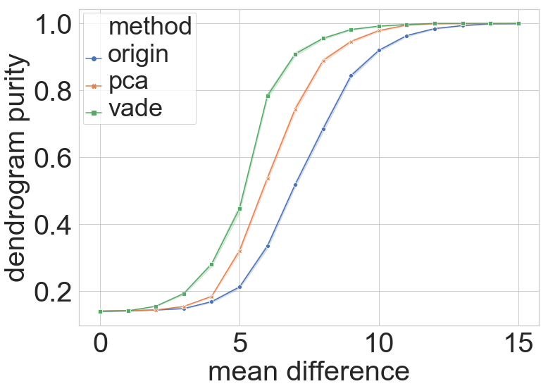
These results and arguments indeed justify our motivation for combining VaDE with Ward’s method. To further demonstrate our approach’s power, we experimentally evaluate the clustering performance of three methods on high-dimensional equally separated Gaussian mixtures – the vanilla Ward’s method, the PCA-Ward combination, and the VaDE-Ward combination. As shown in Figure 2(a), in terms of the dendrogram purity, Ward’s method with VaDE pre-processing tops the other two, for nearly every mean-separation level. In terms of the final clustering result in the (projected) space, Figures 2(b) to 2(d) clearly shows the advantage of the VaDE-Ward method as it significantly enlarges the separation among different clusters while making much fewer mistakes in the clustering accuracy.
Next, we show that given the exact recovery in Theorem 1 and some mild cluster separation conditions, Ward’s method recovers the target hierarchy.
For any index set and the corresponding Gaussian components , denote by the total weight , and by the union of sample points from these components. We say that a collection of nonempty subsets of form a hierarchy of order over if there exists a index set sequence for such that i) for every , the set partitions ; ii) is the union of ; iii) for every and , we have for some .
For any sample size and Gaussian component , denote by , which upper bounds the radius of the corresponding sample cluster, with high probability. The triangle inequality then implies that for any , the distance between a point in the sample cluster of and that of is at most , and at least . Naturally, we also define and for any .
Theorem 2.
There exists an absolute constant such that the following holds. Suppose we are given a sample of size from a -mixture of spherical Gaussians that satisfy the separation conditions and the sample size lower bound in Theorem 1, and suppose that there is an underlying hierarchy of the Gaussian components satisfying
where . Then, Ward’s method recovers the underlying hierarchy with probability at least .
The above theorem resembles Theorem 1, with separation conditions comparing the cluster radiuses with the inter-cluster distances at different hierarchy levels. Informally, the theorem states that if the clusters in each level of the hierarchy are well-separated, Ward’s method will be able to recover the correct clustering of that level, and hence also the entire hierarchy.
5 Experiments
We empirically determine which embedding method produces the best results for dendrogram purity and Moseley-Wang’s objective. We use Ward’s method for clustering after embedding (Appendix C has other algorithms). We provide results for our synthetic model (BTGM) and three real datasets.
Set-up and methods. We compare VaDE against PCA (linear baseline) and a standard VAE (non-linear baseline). All the embedding methods are trained on the whole dataset. Then we run Ward’s method on the sub-sampled embedded data and the original data to get the dendrograms. In the experiments, we only use 25 classes from CIFAR-100 that fall into one of the five superclasses “aquatic animals”, “flowers”, “fruits and vegetables”, “large natural outdoor scenes” and “vehicle1”. We call it CIFAR-25, and we also use CIFAR-25-s to refer to the images labeled with the five superclasses. We average the results over 100 runs, each with 10k random samples from each dataset (except 20newsgroup where we use all 18k samples). Details in Appendix C.
Synthetic Data (BTGM). We vary the depth and margin of the BTGM evaluate different regimes of hierarchy depth and cluster separation. After generating different means for the BTGM, we shift all the non-zero entries of the first means to an arbitrary location. The goal is to show that this simple non-linear transformation is challenging for linear embedding methods (i.e., PCA), while preserving the hierarchical structure. To generate the dataset of clusters with shifted means, we sample 2000 points from each Gaussian distributions of the BTGM of height h such that . Then, we set the embedding dimension of PCA, VAE and VaDE to be .
Dendrogram Purity (DP). We compute the DP of various methods using (3). We construct ground truth clusters either from class labels of real datasets or from the leaf clusters of the BTGM model.
Moseley-Wang’s Objective (MW). To evaluate the MW objective in (2), we need pairwise similarities . For classification datasets, we let to be the indicator function for point and being in the same class. When there are hierarchical labels, we instead define , where denotes the label for point at the level of the hierarchical tree from top to bottom. We measure the ratio achieved by various methods to the optimal MW value opt that we compute as follows. For flat clusters, the optimal MW value is obtained by first merging points in the same clusters, then building a binary tree on top of the clusters. When there are hierarchical labels, we compare against the optimal tree with ground truth levels.

5.1 Results
Results on Synthetic Data. Table 3(b) presents the results of the synthetic experiments. We set the margin of the BTGM to be 8 while varying the depth, so the closest distance between the means of any two Gaussian distributions is 8. We also set the embedding dimension to be , which is the intrinsic dimensionality of the pre-shifted means. As Table 3(b) shows, the combination of embedding with VaDE and then clustering with Ward’s method improves the dendrogram purity and Moseley-Wang’s objective in all settings. VaDE fully utilizes the -dimensional latent space. On the other hand, embedding with PCA or VAE is actually detrimental to the two objectives compared to the original data. We conjecture that PCA fails to resolve the non-linear shifting of the underlying means. In general, using a linear embedding method will likely lead to a drop in both DP and MW for this distribution. Similarly, VAE does not provide sufficient separation between clusters.
Results on Real Data. Tables 2 and 3 report the values of the DP and MW objectives on real datasets. We observe that for MNIST, using the VaDE embedding improves DP and MW significantly compared to other embeddings, and applying the transformation further leads to an increased value of both objectives. Compared to PCA and VAE, we see that VaDE also has lower variance in the clustering results over randomly sampled subsets from the MNIST dataset. The results on the Reuters dataset show that VaDE plus the rescaling transformation is also suitable for text data, where it leads to the best performance. In the CIFAR-25 experiments, we see only a modest improvement with VaDE when evaluating with all 25 classes. It seems that a large number of real clusters may be a limitation of the VaDE embedding, and this deserves additional attention. On the other hand, when restricting to the five superclass labels, the improvement on CIFAR-25-s increases. We hypothesize that VaDE generates a latent space that encodes more of the high level structure for the CIFAR-25 images. This hypothesis can be partially verified by the qualitative evaluation in Figure 3. A trend consistent with the synthetic experiments is that PCA and VAE are not always helpful embeddings for hierarchical clustering with Ward’s method. Overall, VaDE discovers an appropriate embedding into Euclidean space based on its GMM prior that improves the clustering results.
| = 8 ( = 3) | = 16 ( = 4) | = 32 ( = 5) | |
|---|---|---|---|
| Original | 0.798 .020 | 0.789 .017 | 0.775 .016 |
| PCA | 0.518 .002 | 0.404 .003 | 0.299 .003 |
| VAE | 0.619 .030 | 0.755 .019 | 0.667 .012 |
| VaDE | 0.943 .011 | 0.945 .001 | 0.869 .013 |
| 0.960 0.004 | 0.980 0.002 | 0.989 0.001 |
| 0.909 0.001 | 0.913 0.004 | 0.936 0.001 |
| 0.791 0.028 | 0.898 0.017 | 0.969 0.011 |
| 0.990 0.020 | 0.994 0.001 | 0.991 0.001 |
| Reuters | MNIST | CIFAR-25-s | CIFAR-25 | |
|---|---|---|---|---|
| Original | 0.535 .023 | 0.478 .025 | 0.280 .009 | 0.110 .005 |
| PCA | 0.587 .021 | 0.472 .025 | 0.275 .007 | 0.108 .004 |
| VAE | 0.468 .027 | 0.495 .030 | 0.238 .004 | 0.082 .003 |
| VaDE | 0.650 .015 | 0.803 .021 | 0.287 .009 | 0.120 .003 |
| VaDE + Trans. | 0.672 .009 | 0.886 .015 | 0.300 .008 | 0.128 .004 |
| Reuters | MNIST | CIFAR-25 | |
|---|---|---|---|
| Original | 0.654 .025 | 0.663 .014 | 0.438 .005 |
| PCA | 0.679 .021 | 0.650 .037 | 0.435 .007 |
| VAE | 0.613 .027 | 0.630 .034 | 0.393 .004 |
| VaDE | 0.745 .025 | 0.915 .017 | 0.455 .003 |
| VaDE + Trans. | 0.768 .012 | 0.955 .005 | 0.472 .002 |
5.2 Discussion
Theoretical insights. In Theorems 1 and 2, we showed that Ward’s method recovers the hierarchical clustering when the Gaussian means are separated in Euclidean distance. Since VaDE uses a GMM prior, this is a natural metric for the embedded space. As the rescaling increases the separation, we suppose that the embedded vectors behave as if they are approximately sampled from a distribution satisfying the conditions of the theorems. Thus, our theoretical results justify the success of the embedding in practice, where we see that VaDE+Transformation performs the best on many datasets.
Recovering planted and real hierarchies. The synthetic reuslts in Table 3(b) exhibit the success of the VaDE+Transformation method to recover the underlying clusters and the planted hierarchy. This trend holds while varying the number of clusters and depth of the hierarchy. Qualitatively, we find that VaDE can “denoise” the sampled points when the margin does not suffice to guarantee non-overlapping clusters. This enables Ward’s method to achieve a higher value of DP and MW than running the algorithm on the original data. If the hierarchy is not encoded in Euclidean space, e.g., MNIST or CIFAR-25, then VaDE provides good embeddings from which Ward’s method can recover the hierarchy. In many cases, PCA and VAE are unable to find a good embedding.
Rescaling helps. The rescaling transformation, although simple, leads to consistently better results for both DP and MW on multiple real datasets. In practice, the data distributions are correlated and overlapping, without clear cluster structure in high-dimensional space. The VaDE embedding leads to more concentrated clusters, and the rescaling transformation enlarges the separation enough for Ward’s method to recover what is learned by VaDE. In the synthetic experiments, the latent distributions learned by VaDE are already well-separated, so the rescaling is not necessary in this case. In the future, it may be beneficial to explore transformations that depend on the whole hierarchy.
6 Conclusion
We investigated the effectiveness of embedding data in Euclidean space to improve unsupervised hierarchical clustering methods. We saw that rescaling the VaDE latent space embedding, and then applying Ward’s linkage-based method, leads to the best results for dendrogram purity and the Moseley-Wang objective on many datasets. To better understand the VaDE embedding, we proposed a planted hierarchical model using Gaussians with separated means. Theoretically, we proved that Ward’s method recovers both the clustering and the hierarchy with high probability in this model.
While we focus on embedding using variational autoencoders, an open direction for further research could involve embedding hierarchical structure using other representation learning methods agarwal2007generalized; borg2005modern; caron2018deep; chierchia2019ultrametric; mishne2019diffusion; nina2019decoder; salakhutdinov2012one; tsai2017learning; yadav2019supervised. Another direction is to better understand the differences between learned embeddings, comparison-based methods, and ordinal relations emamjomeh2018adaptive; ghoshdastidar2019foundations; kazemi2018comparison; jamieson2011low. Finally, it would be worth exploring the use of approximate clustering methods to improve the running time abboud2019subquadratic; kobren2017hierarchical; rashtchian2017clustering.
Appendix A Proof of the Theorems
The next two lemmas provide tight tail bounds for binomial distributions and spherical Gaussians.
Lemma 1 (Concentration of binomial random variables).
[chung2006complex] Let be a binomial random variable with mean , then for any ,
and for any ,
Lemma 2 (Concentration of spherical Gaussians).
[Gaussian2016notes] For a random distributed according to a spherical Gaussian in dimensions (mean and variance in each direction), and any ,
Lemma 3 (Optimal clustering through Ward’s method).
[grosswendt2019analysis, grosswendt_2020] Let be a collection of points with underlying clustering , such that the corresponding cluster mean values satisfy for all , where is the maximum ratio between cluster sizes. Then Ward’s method recovers the underlying clustering.
Now we are ready to prove Theorem 1.
Proof of Theorem 1.
First, for each component in the mixture, we determine the associated number of sample points. This is equivalent to drawing a size- sample from the weighting distribution that assigns to each . The number of times each symbol appearing in the sample, which we refer to as the (sample) multiplicity of the symbol, follows a binomial distribution with mean . By Lemma 1, the probability that an arbitrary multiplicity is within a factor of from its mean value is at least . Hence, for , the union bound yields that this deviation bound holds for all symbols with probability at least .
Second, given the symbol multiplicities, we draw sample points from each component correspondingly. Consider the -th component with mean . Then, by Lemma 2, every sample point from this component deviates (under Euclidean distance) from by at most , with probability at least . Again, the union bound yields that this deviation bound holds for all components and all sample points with probability at least .
Third, by the above reasoning and , with probability at least and for all ,
-
1.
the sample size associated with the -th component is between and ;
-
2.
every sample point from the -th component deviates from by at most .
Therefore, if further for all , the sample points will form well-separated clusters according to the underlying components. In addition, the first assumption ensures that the maximum ratio between cluster sizes is at most , and the second assumption implies that for any ,
-
1.
the -th cluster the distance between the mean to any point in it is at most ;
-
2.
the empirical means of the -th and -th clusters are separated by at least
Finally, applying Lemma 3 completes the proof of the theorem. ∎
Next, we move to the proof of Theorem 2. Let us first recap what the theorem states.
Theorem 2.
There exists an absolute constant such that the following holds. Suppose we are given a sample of size from a -mixture of spherical Gaussians that satisfy the separation conditions and the sample size lower bound in Theorem 1, and suppose that there is an underlying hierarchy of the Gaussian components satisfying
where . Then, Ward’s method recovers the underlying hierarchy with probability at least .
Proof of Theorem 2.
By the proof of Theorem 1, for any sample size and Gaussian component , the quantity upper bounds the radius of the corresponding sample cluster, with high probability. Here, the term “radius” is defined with respect to the actual center .
The triangle inequality then implies that for any , the distance between a point in the sample cluster of and that of is at most , i.e., the sum of the distance between the two centers and the radiuses of the two clusters, and at least .
More generally, for any non-singleton clusters represented by , the distance between two points and is at most , and at least . In particular, for , quantity upper bounds the diameter of cluster .
Furthermore, by the proof of Theorem 1, given the exact recovery of the Gaussian components, the ratio between the sizes of any two clusters (at any level), say and , differs from the ratio between their weights, , by a factor of at most . Hence, the quantity essentially characterizes the maximum ratio between the sample cluster sizes at level of the hierarchy.
With the above reasoning, Lemma 3 naturally completes the proof of the theorem. Intuitively, this shows that if the clusters in each level of the hierarchy are well-separated, Ward’s method will be able to recover the correct clustering of that level, and hence also the entire hierarchy. ∎
Appendix B Optimally of Theorem 1
Below, we illustrate the hardness of improving the theorem without preprocessing the data, e.g., applying an embedding method to the sample points, such as VaDE or PCA.
Separation conditions.
As many other commonly used linkage methods, the behavior and performance of Ward’s method depend on only the inter-point distances between the observations. For optimal-clustering recovery through Ward’s method, a natural assumption to make is that the distances between points in the same cluster is at most that between disjoint clusters. Consider a simple example where we draw sample points from a uniform mixture of two standard -dimensional spherical Gaussians and with mean separated by a distance . Then, with a probability, we will draw two sample points from , say , and one sample point from , say . Conditioned on this, the reasoning in Section 2.8 of [blum2020foundations] implies that, with high probability,
Hence, the assumption that points are closer inside the clusters translates to
Furthermore, if one requires the inner-cluster distance to be slightly smaller than the inter-cluster distance with high probability, say , where is a small constant,
Therefore, the mean difference between the two Gaussians should exhibit a linear dependence on .
In addition, for a standard -dimensional spherical Gaussian, Theorem 2.9 in [blum2020foundations] states that for any , all but at most of its probability mass lies within . Hence, if we increase the sample size from to , correctly separating the points by their associated components requires an extra term in the mean difference.
Sample-size lower bound.
In terms of the sample size , Theorem 1 requires . For Ward’s method to recover the underlying -component clustering with high probability, we must observe at least one sample point from every component of the Gaussian mixture. Clearly, this means that the expected size of the smallest cluster should be at least , implying . If we have , this reduces to a weighted version of the coupon collector problem, which calls for a sample size in the order of by the standard results [feller1968introduction].
Appendix C More Experimental Details
Network Architecture. The architecture for the encoder and decoder for both VaDE and VAE are fully-connected layers with size -2000-500-500- and -500-500-2000-, where is the hidden dimension for the latent space , and is the input dimension of the data in . These settings follow the original paper of VaDE [jiang2017variational]. We use Adam optimizer on mini-batched data of size 800 with learning rate 5e-4 on all three real datasets. The choices of the hyper-parameters such as and will be discussed in the Sensitivity Analysis.
Computing Dendrogram Purity. For every set of points sampled from the dataset (e.g. we use for MNIST, CIFAR-25), we compute the exact dendrogram purity using the formula 3. We then report the mean and standard variance of the results by repeating the experiments 100 times.
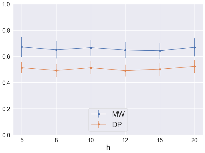
Sensitivity Analysis. We check the sensitivity of VAE and VaDE to its hyperparameters and in terms of DP and MW. We also check the sensitivity of rescaling factor applied after the VaDE embedding. The details are presented in Figure 4, 5, and 6.


Comparing Linkage-Based Methods. Table 4 shows the DP and MW results for several linkage-based variations, depending on the function used to determine cluster similarity. Overall, we see that Ward’s method performs the best on average. However, in some cases, the other methods do comparably.
| Dendro. Purity | M-W objective | Dendro. Purity | M-W objective | |
|---|---|---|---|---|
| Single | 0.829 0.038 | 0.932 0.023 | 0.260 0.005 | 0.419 0.006 |
| Complete | 0.854 0.040 | 0.937 0.024 | 0.293 0.008 | 0.451 0.016 |
| Centroid | 0.859 0.035 | 0.949 0.019 | 0.284 0.008 | 0.453 0.009 |
| Average | 0.866 0.035 | 0.948 0.023 | 0.295 0.005 | 0.462 0.006 |
| Ward | 0.870 0.031 | 0.948 0.025 | 0.300 0.008 | 0.465 0.011 |
| MNIST | CIFAR-100 |


Dataset Details. We conduct the experiments on our synthetic data from BTGM as well as real data benchmarks: Reuters , MNIST [MNIST] and CIFAR-100 [CIFAR100]. In the experiments, we only use 25 classes from CIFAR-100 that fall into one of the five superclasses "aquatic animals", "flowers", "fruits and vegetables", "large natural outdoor scenes" and "vehicle1" 111The information of these superclasses can be found in https://www.cs.toronto.edu/ kriz/cifar.html, we call it CIFAR-25. Below we also provide further details on the Digits dataset of handwritten digits 222https://archive.ics.uci.edu/ml/datasets/Optical+Recognition+of+Handwritten+Digits. More details about the number of clusters and other statistics can be found in Table 5.
Rescaling explained. The motivation of rescaling transformation can be explained using Figure 7. (a) shows the tSNE visualization of the VaDE embedding before and after the rescaling transformation. As we can see, each cluster becomes more separated. In (b), we visualize the inter-class distance matrices before and after the transformation. We use blue and black bounding boxes to highlight few superclusters revealed in the VaDE embedding. These high level structures remain unchanged after the rescaling, which is a consequence of property (ii) in Section 3.
| Digits | Reuters | MNIST | CIFAR-25-s | CIFAR-25 | |
|---|---|---|---|---|---|
| # ground truth clusters | 10 | 4 | 10 | 5 | 25 |
| # data for training | 6560 | 680K | 60K | 15K | 15K |
| # data for evaluation | 1000 | 1000 | 2048 | 2048 | 2048 |
| Dimensionality | 64 | 2000 | 768 | 3072 | 3072 |
| Size of hidden dimension | 5 | 10 | 10 | 20 | 20 |
C.1 Digits Dataset
There are few experimental results that evaluate dendrogram purity for the Digits dataset in previous papers. First we experiment using the same settings and same test set construction for Digits as in [monath2019gradient]. In this case, VaDE+Ward achieves a DP of 0.941, substantially improving the previous state-of-the-art results for dendrogram purity from existing methods: the DP of [monath2019gradient] is 0.675, the DP of PERCH [kobren2017hierarchical] is 0.614, and the DP of BIRCH [BIRCH1996] is 0.544. In other words, our approach of VaDE+Ward leads to 26.5 point increase in DP for this simple dataset.
Surprisingly, we find that the test data they used is quite easy, as the DP and MW numbers are substantially better compared to using a random subset as the test set. Therefore, we follow the same evaluation settings as in Section 5 and randomly sampled 100 samples of 1000 data points for evaluation. The results are shown in Table 6. The contrast between the previous test data (easier) versus random sampling (harder) further supports our experimental set-up in the main paper.
| Dendro. Purity | M-W objective | |
|---|---|---|
| Original | 0.820 0.031 | 0.846 0.029 |
| PCA | 0.823 0.028 | 0.844 0.027 |
| VaDE | 0.824 0.026 | 0.840 0.024 |
| VaDE + Trans. | 0.832 0.029 | 0.845 0.024 |

